
TL;DR
This paper explores methods to correctly identify a geometric curve often mistaken for a circle, using elementary and technological approaches suitable for classroom teaching at various educational levels.
Contribution
It introduces novel technological methods with GeoGebra to distinguish the curve from a circle and provides multiple approaches for verification, enhancing geometric understanding.
Findings
Two methods to refute the false impression of the curve as a circle
Two suggestions to formulate correct conjectures
Four rigorous proof techniques for confirmation
Abstract
A popular curve shown in introductory maths textbooks, seems like a circle. But it is actually a different curve. This paper discusses some elementary approaches to identify the geometric object, including novel technological means by using GeoGebra. We demonstrate two ways to refute the false impression, two suggestions to find a correct conjecture, and four ways to confirm the result by proving it rigorously. All of the discussed approaches can be introduced in classrooms at various levels from middle school to high school.
Click any figure to enlarge with its caption.
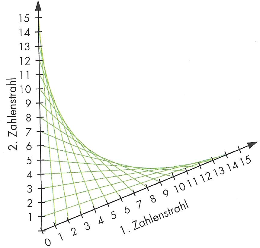 Figure 1
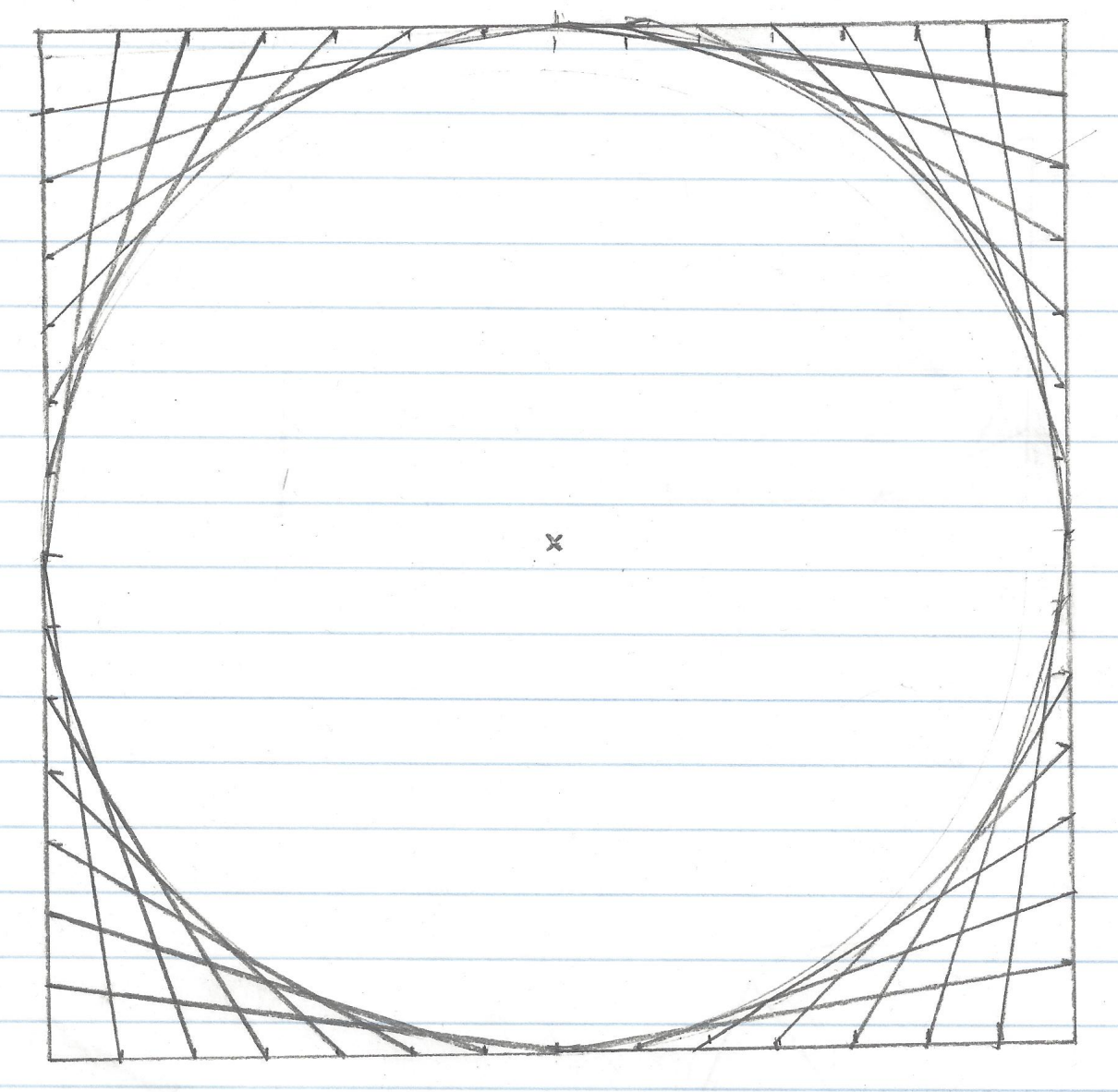 Figure 2
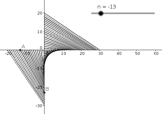 Figure 3
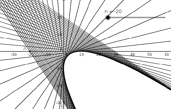 Figure 4
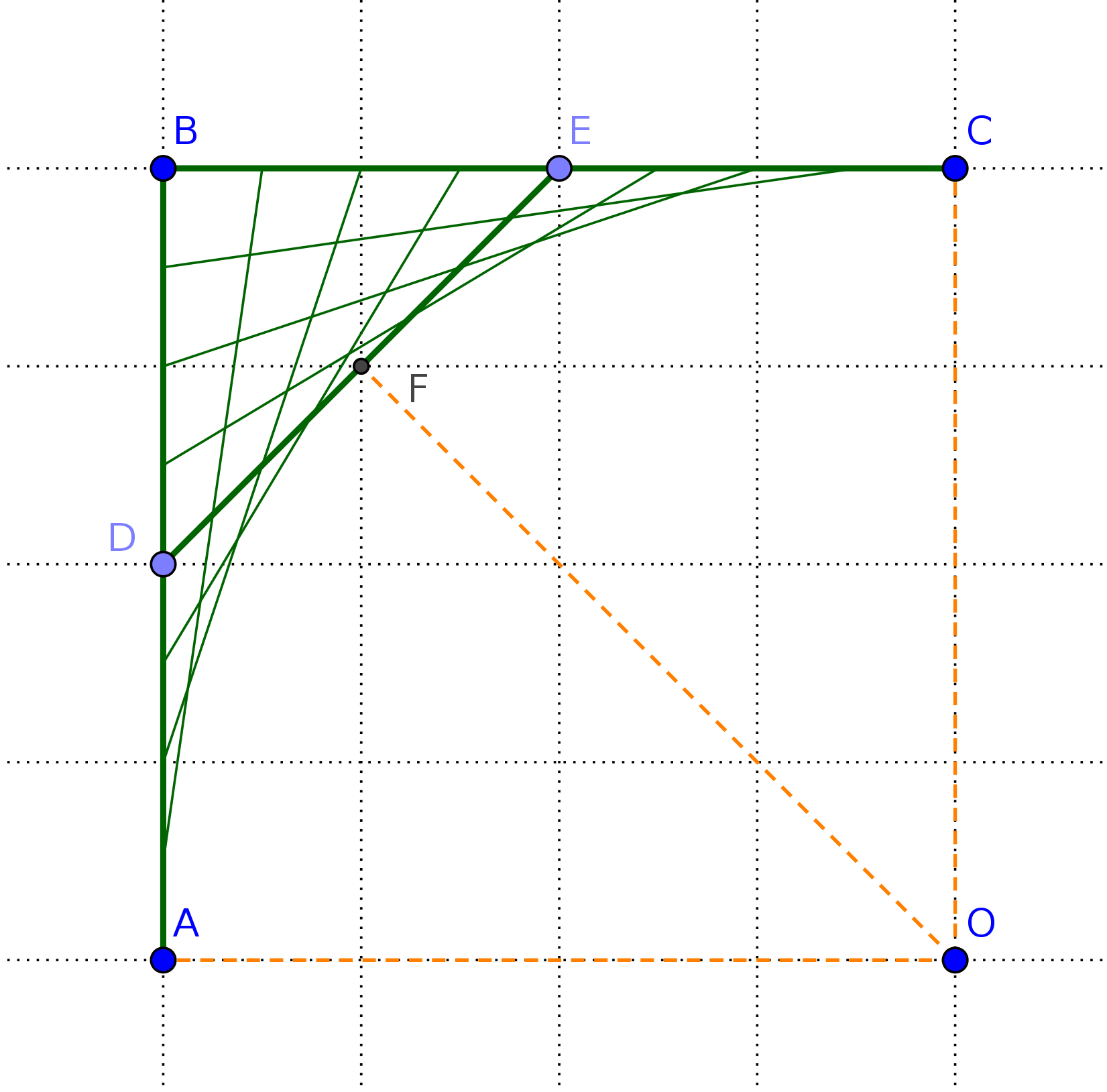 Figure 5
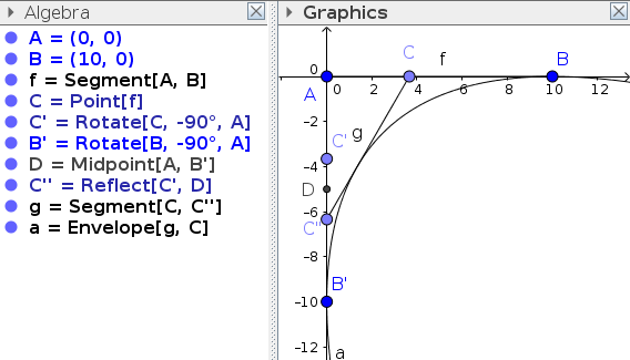 Figure 6
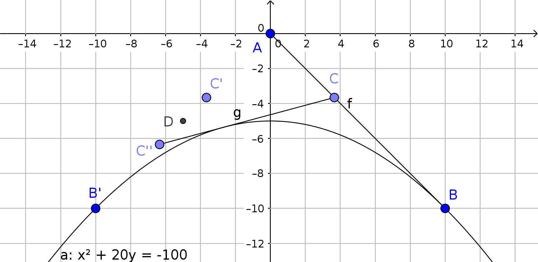 Figure 7
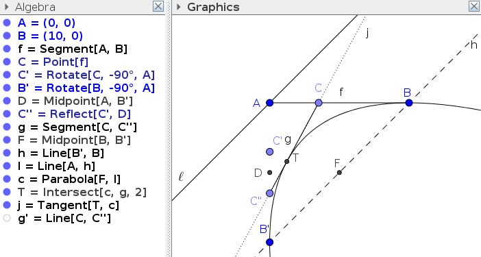 Figure 8
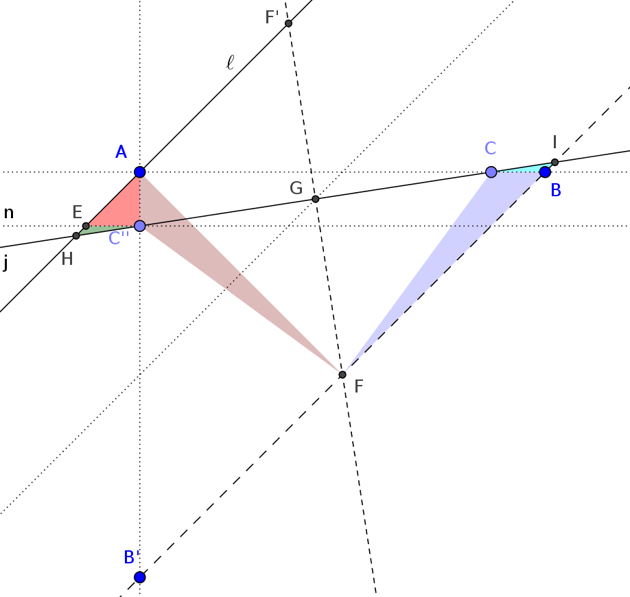 Figure 9
 Figure 10
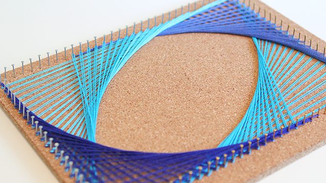 Figure 11
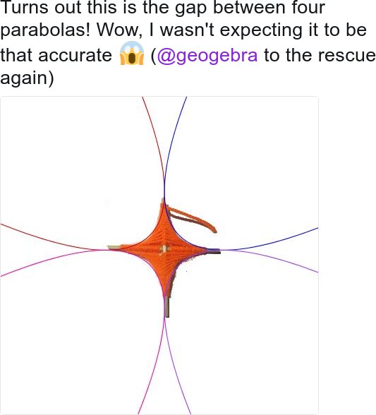 Figure 12
Peer Reviews
No public reviews on file for this paper yet. If you reviewed it on a platform where reviews are public (OpenReview, ICLR, NeurIPS, ICML), you can paste yours below so the community can read it here.
Videos
No videos yet. Explain this paper in a talk, walkthrough, or lecture? Add one.
Taxonomy
TopicsData Management and Algorithms · 3D Modeling in Geospatial Applications · Graph Theory and Algorithms
11institutetext: The Private University College of Education of the Diocese of Linz
Salesianumweg 3, A-4020 Linz, Austria
11email: [email protected]
No, This is not a Circle!
Zoltán Kovács
Abstract
A popular curve shown in introductory maths textbooks, seems like a circle. But it is actually a different curve. This paper discusses some elementary approaches to identify the geometric object, including novel technological means by using GeoGebra. We demonstrate two ways to refute the false impression, two suggestions to find a correct conjecture, and four ways to confirm the result by proving it rigorously.
All of the discussed approaches can be introduced in classrooms at various levels from middle school to high school.
Keywords:
string art, envelope, GeoGebra, computer algebra, computer aided mathematics education, automated theorem proving
1 But it looks like a circle
One possible anti boredom activity is to simulate string art in a chequered notebook, as seen below the title of this paper. This kind of activity is easy enough to do it very early, even as a child during the early school years. The resulting curve, the contour of the “strings”, or more precisely, a curve whose tangents are the strings, is called an envelope.
According to Wikipedia [1], an envelope of a family of curves in the plane is a curve that is tangent to each member of the family at some point.111This definition is however polysemic: the Wikipedia page lists other non-equivalent ways to introduce the notion of envelopes. See [4] for a more detailed analysis on the various definitions. Let us assume that the investigated envelope—below the title of this paper—which is defined similarly as the learner activity in Fig. 1, is a circle. In the investigated envelope it will be assumed that a combination of 4 simple constructions is used, the axes are perpendicular, and the sums of the joined numbers are 8. To be more general, these sums may be changed to different (but fixed) numbers. These sums will be denoted by to recall the distance of the origin and the furthermost point for the exterior strings.
By using the assumption of the circle property, in our case the family of the strings must be equally far from the center of the circle. This needs to be true because the circle is the only curve whose tangents are equally far from the center. Due to symmetry of the 4 parts of the figure, the only possible center for the circle is the midpoint of the figure. Let us consider the top-left part of the investigated figure (Fig. 2). On the left and the top the strings and have the distance from center . On the other hand, the diagonal string has distance from the assumed center, according to the Pythagorean theorem. This latter distance is approximately , that is, more than . Consequently, the curve cannot be an exact circle. That is, it is indeed not a circle.
In schools the Pythagorean theorem is usually introduced much later than the students are ready to simply measure the length of and by using a ruler. The students need to draw, however, a large enough figure because the difference between and is just about 6%. Actually, both methods obviously prove that the curve is different from a circle, and the latter one can already be discussed at the beginning of the middle school.
2 OK, it is not a circle—but what is it then?
Let us continue with a possible classroom solution of the problem. Since the strings are easier to observe than the envelope, it seems logical to collect more information about the strings. Extending the definition of the investigated envelope by continuing the strings to both directions, we learn how the slope of the strings changes while continuing the extension more and more (Fig. 3). Here we remark that the top-left part of the investigated envelope is now mirrored about the first axis (cf. Fig. 1), therefore not the sums but the differences will be constant, namely .
The strings in the extension support the idea that the tangents of the curve, when is large enough, are almost parallel to the line . This observation may refute the opinion that the curve is eventually a hyperbola (which has two asymptotes, but they are never parallel).
On the other hand, by changing the segments in Fig. 3 to lines an obvious conjecture can be claimed, that is, the curve is a parabola (Fig. 4). Thus the observed curve must be a union of 4 parabolic arcs.
3 We have a conjecture—can we verify that?
A GeoGebra applet in Fig. 5 can explicitly compute the equation of the envelope and plot it accurately. (See [4] for a detailed survey on the currently available software tools to visualize envelopes dynamically.) For technical reasons a slider cannot be used in this case—instead a purely Euclidean construction is required as shown in the figure. Free points and are defined to set the initial parameters of the applet, and finally segment describes the family of strings. The command Envelope[,] will then produce an implicit curve, which is in this concrete case .
GeoGebra uses heavy symbolic computations in the background to find this curve [5]. Since they are effectively done, the user may even drag points and to different positions and investigate the equation of the implicit curve. They are recomputed quickly enough to have an overview on the resulted curve in general—they are clearly quadratic algebraic curves in variables and .
Without any deeper knowledge of the classification of algebraic curves, of course, young learners cannot really decide whether the resulted curve is indeed a parabola. Advanced learners and maths teachers could however know that all real quadratic curves are either circles, ellipses, hyperbolas, parabolas, a union of two lines or a point in the plane. As in the above, we can argue that the position of the strings as tangents support only the case of parabolas here.
On the other hand, for young learners we can still find better positions for and . It seems quite obvious that the curve remains definitely the same (up to similarity), so it is a free choice to define the positions of and . By keeping in the origin and putting on the line we can observe that the parabola is in the form which is the usual way how a parabola is introduced in the classroom. (In our case actually .) For example, when , the implicit curve is , and this can be easily converted to (Fig. 6).
This result is computed by using precise algebraic steps in GeoGebra. One can check these steps by examining the internal log—in this case 16 variables and 11 equations will be used including computing a Jacobi determinant and a Gröbner basis when eliminating all but two variables from the equation system. That is, GeoGebra actually provides a proof, albeit its steps remain hidden for the user. (Showing the detailed steps when manipulating on an equation system with so many variables makes no real sense from the educational point of view: the steps are rather mechanical and may fill hundreds of pages.)
As a conclusion, it is actually proven that the curve is a parabola. Of course, learners may want to understand why it that curve is.
4 Proof in the classroom
Here we provide two simple proofs on the fact that the envelope is a parabola in Fig. 6. The first method follows [6].
We need to prove that segment is always a tangent of the function . First we compute the equation of line to find the intersection point of and the parabola.
We recognize that if point , then point .
Now we have two possible approaches to continue.
Since line has an equation in form , we can set up equations for points and as follows:
[TABLE]
and
[TABLE]
Now (1)(2) results in and thus, by using again we get .
Second, to obtain intersection point we consider equation which can be reformulated to search the roots of quadratic function . If and only if the discriminant of this quadratic expression is zero, then is a tangent. Indeed, the determinant is which is, after inserting and , obviously zero. 2. 2.
Another method to show that is a tangent of the parabola is to use elementary calculus. School curricula usually includes computing tangents of polynomials of the second degree.
Let . Now the steepness of the tangent of the parabola in is . It means that the equation of the tangent is , here can be computed by using and , that is . The equation of the tangent is consequently
[TABLE]
Let us assume now that and are the intersections of the tangent and the lines and , respectively. The -coordinate of can be found by putting in (3), it is
[TABLE]
On the other hand, the -coordinate of can be found by putting in (3), it is
[TABLE]
By using some basic algebra it can be confirmed that , that is is indeed a string.
The second proof is technically longer than the first one but still achievable in many classrooms.
Both approaches are purely analytical proofs without any knowledge of the synthetic definition of a parabola. The fact is that in many classrooms, unfortunately, the synthetic definition is not introduced or even mentioned.
5 A synthetic approach
In the schools where the synthetic definition of a parabola is also introduced, the most common definition is that it is the locus of points in the plane that are equidistant from both the directrix line and the focus point .
5.1 An automated answer
Without any further considerations it is possible to check (actually, prove) that the investigated curve is a parabola also in the symbolic sense. To achieve this result one can invoke GeoGebra’s Relation Tool [7] after constructing the parabola synthetically as seen in Fig. 7.
Here the focus point is the midpoint of , and the directrix line is a parallel line to through . This piece of information should be probably kept secret by the teacher—the learners could find them on their own. Now to check if the string is indeed a tangent of the parabola the tangent point has been created as an intersection of the string and the parabola. Also a tangent line has been drawn, and finally line which is the extension of segment to a full line. At this point it is possible to compare and by using the Relation Tool.
The Relation Tool first compares the two objects numerically and reports that they are equal. By clicking the “More” button the user obtains the symbolic result of the synthetic statement (Fig. 8).
We recall that despite the construction was performed synthetically, the symbolic computations were done after translating the construction to an algebraic setup. Thus GeoGebra’s internal proof is again based on algebraic equations and still hidden for the user. But in this case we indeed have a general proof for each possible construction setup, not for only one particular case as for the Envelope command.
5.2 A classical proof
Finally we give a classical proof to answer the original question. Here every detail uses only synthetic considerations.
The first part of the proof is a well known remark on the bisection property of the tangent. That is, by reflecting the focus point about any tangent of the parabola the mirror image is a point of the directrix line. (See e.g. [6], Sect. 3.1 for a short proof.) Clearly, it is sufficient to show that the strings have this kind of bisection property: this will result in confirming the statement.
In Fig. 9 the tangent to the parabola is denoted by . Let be the mirror image of about . We will prove that . Let denote the intersection of and . Clearly and are right because of the reflection.
By construction and are congruent. Thus . Moreover, is isosceles and is its bisector at , in addition, .
Let denote a parallel line to through . Let be the intersection of and . Also let be the intersection of and , and let be the intersection of and the line . Since and are parallel, moreover and are also parallel, and (because is actually the rotation of around by 90 degrees), we conclude that and are congruent. This means that .
That is, using also , must be the midpoint of , thus lies on the mid-parallel of and . As a consequence, reflecting about the resulted point is surely a point of line .
6 Conclusion
An analysis of the string art envelope was presented at different levels of mathematical knowledge, by refuting a false conjecture, finding a true statement and then proving it with various means.
Discussion of a non-trivial question by using different means can give a better understanding of the problem. What is more, reasoning by visual “evidence” can be misleading, and only rigorous (or rigorous but computer based) proofs can be satisfactory.
It should be noted that the parabola property of the string art envelope is well known in the literature on Bezier curves, but usually not discussed in maths teacher trainings. The de Casteljeau algorithm for a Bezier curve of degree 2 is itself a proof that the curve is a parabola. (See [9, 10] for more details.) Also among maths professionals this property seems rarely known. A recent example of a tweet of excitement is from February 2017 (Fig. 10).
On the other hand, our approach highlighted the classroom introduction of the string art parabola, and suggested some very recent methods by utilizing computers in the middle and high school to improve the teacher’s work and the learners’ skills.
Lastly, we remark that the definition of the string art envelope looks similar to the envelope of other family of lines. For example, the envelope of the sliding ladder results in a different curve, the astroid [1, 12, 13], a real algebraic curve of degree 6. While “physically” that is easier to construct (one just needs a ladder-like object, e. g. a pen), the geometric analysis of that is more complicated and usually involves partial derivatives. (See also [1] on a proof for identifying the string art parabola by using partial derivatives.)
Acknowledgments
The author thanks Tomás Recio and Noël Lambert for comments that greatly improved the manuscript.
The introductory figure was drawn by Benedek Kovács (12), first grade middle school student.
The reference list from the paper itself. Each links out to its DOI / PubMed record.
- 1[1] Wikipedia: Envelope (mathematics) — Wikipedia, The Free Encyclopedia (2016) [Online; accessed 27-April-2017].
- 2[2] Boxhofer, E., Hubert, F., Lischka, U., Panhuber, B.: mathemati X. Veritas, Linz (2013)
- 3[3] Morgan, S.: Math + art = string art. e How Mom Blog (2013) http://www.ehow.com/ehow-mom/blog/math-art-string-art/ .
- 4[4] Botana, F., Recio, T.: Computing envelopes in dynamic geometry environments. Annals of Mathematics and Artificial Intelligence (2016) 1–18
- 5[5] Kovács, Z.: Real-time animated dynamic geometry in the classrooms by using fast Gröbner basis computations. Mathematics in Computer Science 11 (2017)
- 6[6] Botana, F., Kovács, Z.: New tools in Geo Gebra offering novel opportunities to teach loci and envelopes. Co RR abs/1605.09153 (2016)
- 7[7] Kovács, Z.: The Relation Tool in Geo Gebra 5. In Botana, F., Quaresma, P., eds.: Automated Deduction in Geometry: 10th International Workshop, ADG 2014, Coimbra, Portugal, July 9-11, 2014, Revised Selected Papers. Springer International Publishing, Cham (2015) 53–71
- 8[8] Kovács, Z., Recio, T., Vélez, M.P.: Geo Gebra Automated Reasoning Tools. A Tutorial. A Git Hub project (2017) https://github.com/kovzol/gg-art-doc .