Computation of Induced Orthogonal Polynomial Distributions
Akil Narayan

TL;DR
This paper introduces a stable, spectrally-accurate algorithm for computing distribution functions of induced orthogonal polynomial measures, enabling efficient sampling crucial for advanced polynomial approximation methods.
Contribution
The authors present a novel, robust algorithm for computing and sampling from induced orthogonal polynomial distributions, with implementation available as open-source code.
Findings
Stable computation for polynomial degrees up to 1000
Efficient sampling method for induced distributions
Application to multivariate polynomial approximation
Abstract
We provide a robust and general algorithm for computing distribution functions associated to induced orthogonal polynomial measures. We leverage several tools for orthogonal polynomials to provide a spectrally-accurate method for a broad class of measures, which is stable for polynomial degrees up to at least degree 1000. Paired with other standard tools such as a numerical root-finding algorithm and inverse transform sampling, this provides a methodology for generating random samples from an induced orthogonal polynomial measure. Generating samples from this measure is one ingredient in optimal numerical methods for certain types of multivariate polynomial approximation. For example, sampling from induced distributions for weighted discrete least-squares approximation has recently been shown to yield convergence guarantees with a minimal number of samples. We also provide…
Click any figure to enlarge with its caption.
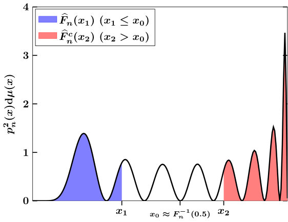 Figure 1
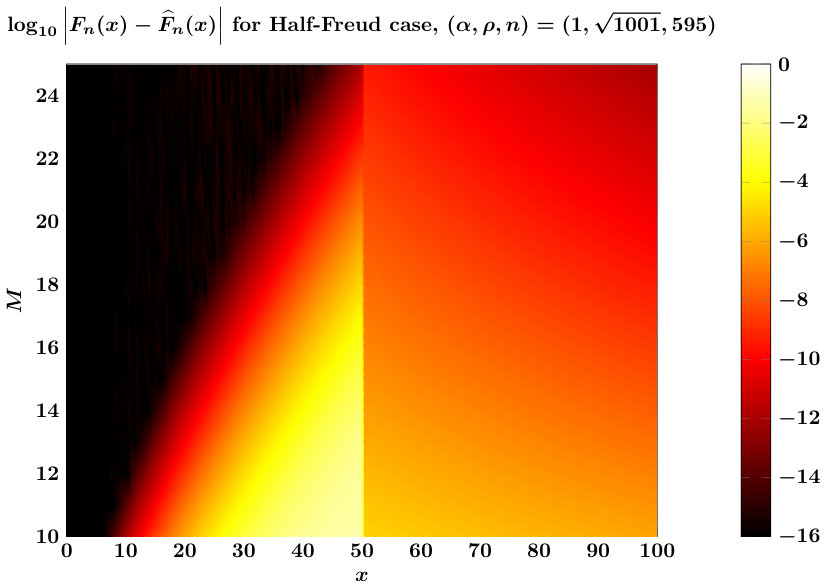 Figure 2
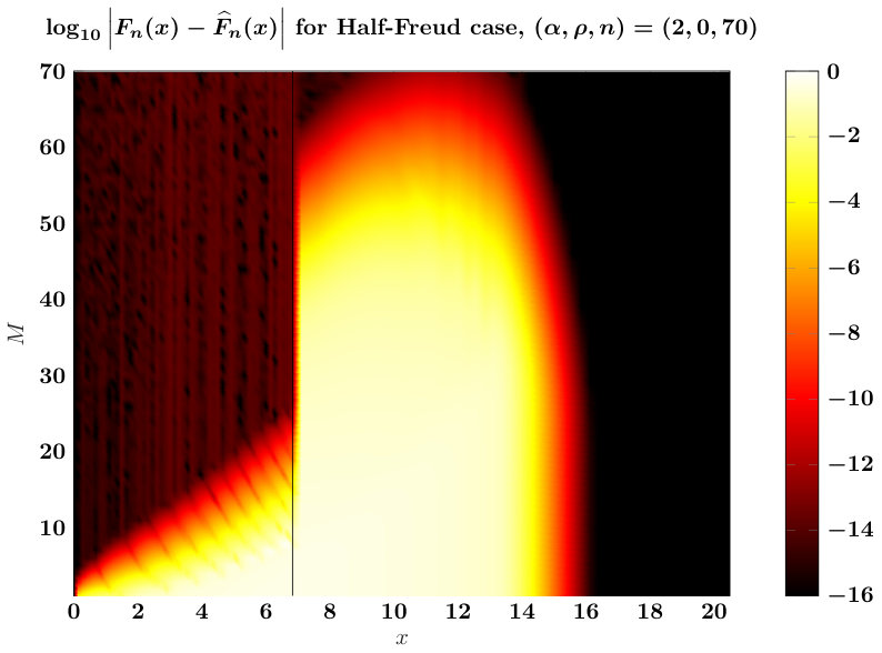 Figure 3
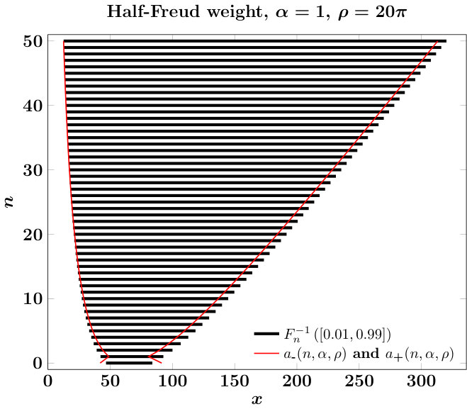 Figure 4
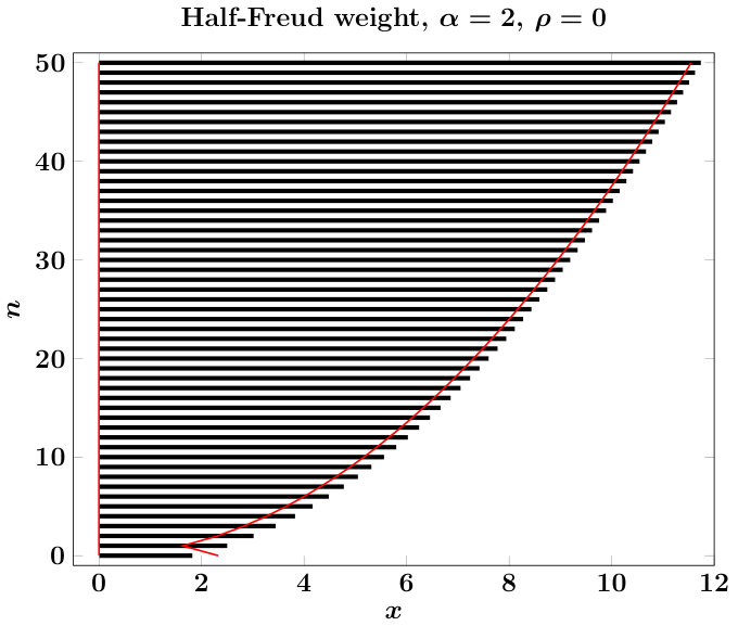 Figure 5
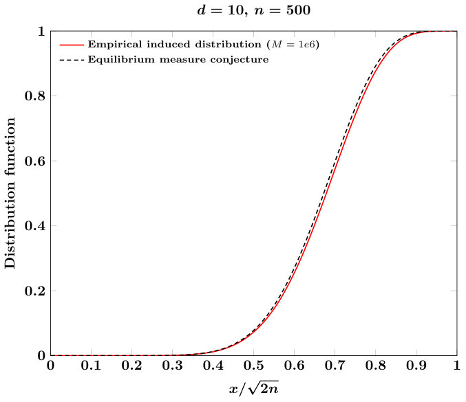 Figure 6
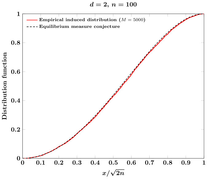 Figure 7
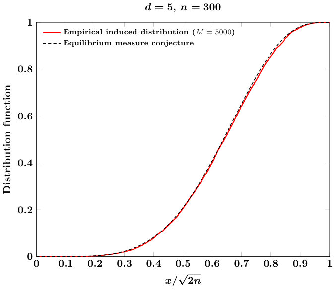 Figure 8
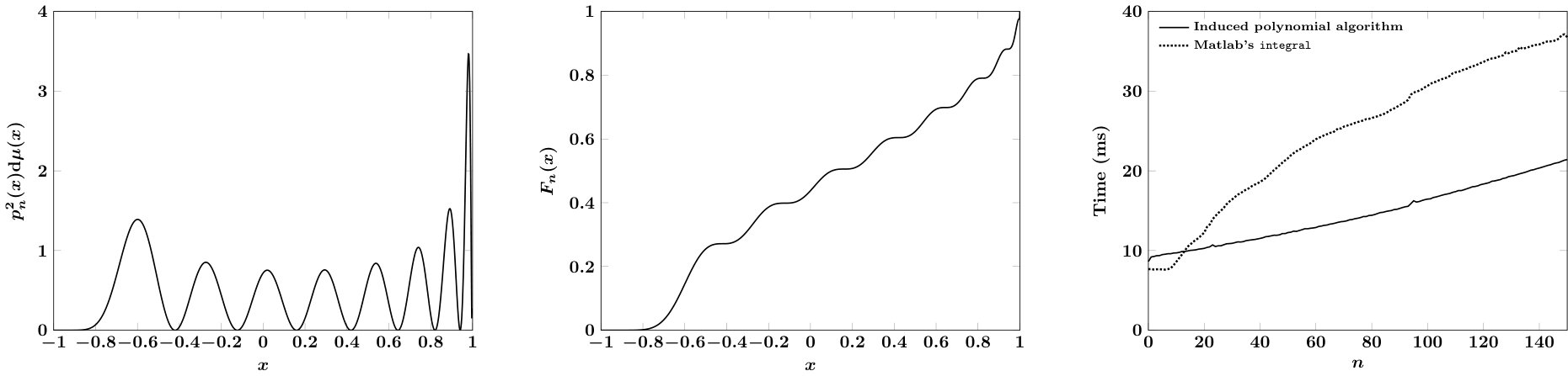 Figure 9
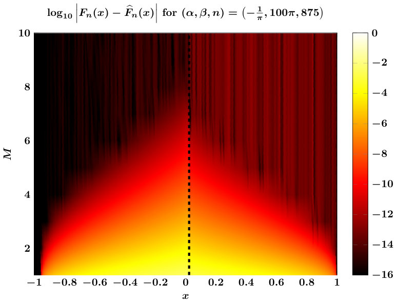 Figure 10
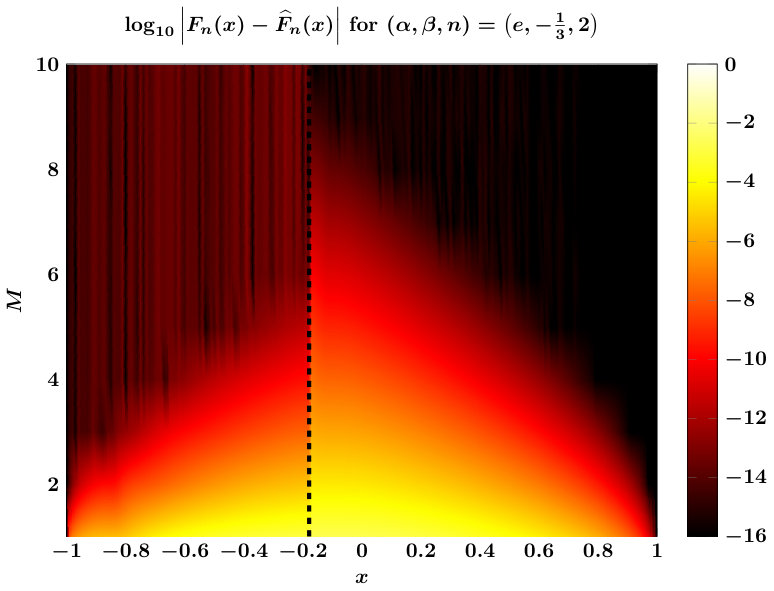 Figure 11
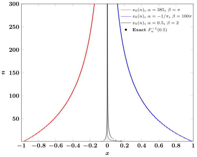 Figure 12
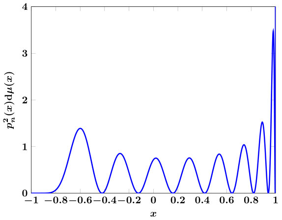 Figure 13
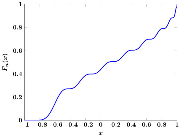 Figure 14
 Figure 15
Peer Reviews
No public reviews on file for this paper yet. If you reviewed it on a platform where reviews are public (OpenReview, ICLR, NeurIPS, ICML), you can paste yours below so the community can read it here.
Videos
No videos yet. Explain this paper in a talk, walkthrough, or lecture? Add one.
x∈R
Note that for large enough . (Appendix B) Polynomial measure modifications: given and its associated three-term recurrence coefficients and , computation of the three-term recurrence coefficients associated with the measures and , defined as
[TABLE]
The sign in is chosen so that is a positive measure.
1. Evaluation of
This section develops computational algorithms for the evaluation of the induced distribution defined in (LABEL:eq:mun-def). These algorithms depend fairly heavily on the form of a Lebesgue density (i.e., a positive weight function) for the measure on , but the ideas can be generalized to various measures. We consider the classes of weights enumerated in Table LABEL:tab:measures:
- •
(Jacobi weights) for with parameters .
- •
(Freud weights) for with parameters , .
- •
(half-line Freud weights) for with parameters , .
The induced distribution for Freud weights can actually be written explicitly in terms of the corresponding induced distribution for half-line Freud weights, so most of the algorithm development concentrates on the Jacobi and half-line Freud cases. The strategy for these two latter cases is essentially the same: with in one of the classes above and fixed, we divide the computation into one of two approximations, depending on the value of . Each approximation is accurate for its corresponding values of . Formally, the algorithm is
[TABLE]
where and represent computational approximations to and , respectively, and are the outputs from the algorithms that we will develop. A pictorial description of this is given in Figure 1 (left). The constant is ideally ; since we cannot know this value a priori, we use potential-theoretic arguments to compute a value approximating the median of ,
[TABLE]
For our choice of , we can provide no estimates for this approximate equality, but empirical evidence in Figure 1 (right) shows that our choices are very close to the real median, uniformly in . The coming sections concentrate on, for each class of mentioned above, specifying and detailing algorithms for and .
1.1. Jacobi weights
We consider computing induced distribution functions for Jacobi measures as defined in Table LABEL:tab:measures. When circumstances are clear, we will write to avoid notational clutter. We seek the distribution function of the induced measure,
[TABLE]
To compute , we specify an approximate median satisfying (4), and construct algorithmic procedures to evaluate (for ) and (for ). Having specified these, we use (3) to compute our approximation to .
1.1.1. Approximating
With , and fixed, consider the measure . Note that this measure is still a Jacobi measure since and . We may rewrite the integrand in (5)
[TABLE]
The quantity under the square brackets on the right-hand side is, in the language of potential theory, a weighed polynomial of degree . One result in potential theory characterizes the “essential” support of this weighted polynomial; in particular, the weighted polynomial decays quickly outside this support. The essential support is an interval, and we take the median of the induced measure to be the centroid of this interval. The essential support of the weighted polynomial above is demarcated by the Mhaskar-Rakhmanov-Saff numbers for the asymmetric weight on . These numbers for this weight are computed explicitly in [23, pp 206-207]. When , this support interval is , with
[TABLE]
Since this is the interval where most of the “mass” of the integral in (5) lies, we set to be the centroid of this interval:
[TABLE]
Note that the definitions of require and to be non-negative. Without mathematical justification, we extend the formula (6) to valid negative values of as well. Figure 1 compares and for certain choices of and .
1.1.2. Computing
First assume that , with defined in (6), and define as
[TABLE]
where is the floor function. We transform the integral (5) over onto the standard interval via the substitution :
[TABLE]
where is a degree- polynomial given by
[TABLE]
where are the zeros of . Since we explicitly know the polynomial roots of , we can absorb the term marked into the measure via linear modifications, and we can likewise absorb the term via quadratic modifications. (See Appendix B.) Thus, define
[TABLE]
which is a modified measure whose recurrence coefficients can be computed via successive application of the linear and quadratic modification methods in Appendix B. Thus,
[TABLE]
The integrand above has a root () or singularity () at ; this root is far outside the interval unless is very large and both and are small. The integrand is therefore a positive, monotonic, smooth function on , taking values between and ; we use an order- -Gaussian quadrature to efficiently evaluate it. With denoting the nodes and weights, respectively, of this quadrature rule, we compute
[TABLE]
The entire procedure is summarized in Algorithm 1. In order to compute for , we use symmetry. Since interchanges the parameters and , then
[TABLE]
Note that if , then . Thus, can be computed via the same algorithm for , but with different values for , , and . This is also shown in Algorithm 1.
Theorem 1.1**.**
With , , and all given, assume that with as in (6). Then the output from Algorithm 1 using an -point quadrature rule satisfies
[TABLE]
where are the three-term recurrence coefficients associated to the -dependent measure defined in (7). The constant is
[TABLE]
Note that on the right-hand side of (11) is explicitly computable once , , , and are fixed, and only the product involving depends on . Furthermore, this last quantity is explicitly computed in Algorithm 1, so that a rigorous error estimate for the algorithm can be computed before its termination. Since , then the estimate (11) also hints at exponential convergence of the quadrature rule strategy, assuming that the factors can be bounded or controlled. We cannot provide these bounds, although we do know the asymptotic behavior as [21, Remark 3.1.10]. Also, since for any then, uniformly in , . Thus, for a fixed we expect that the estimate in Theorem 1.1 behaves like
[TABLE]
showing exponential convergence with respect to . However, we cannot prove this latter statement.
Proof.
The result is a relatively straightforward application of known error estimates for Gaussian quadrature with respect to non-classical weights. We use the notation of Algorithm 1: and denote the -point -Gaussian quadrature nodes and weights, respectively. We start with the Corollary to Theorem 1.48 in [7], stating that if is infinitely differentiable on , then
[TABLE]
for some . Noting that since are the zeros of the degree- -orthogonal polynomial, then
[TABLE]
From (8), the integral we wish to approximate has integrand . Then for any and any ,
[TABLE]
Then
[TABLE]
Since , then
[TABLE]
The result follows by direct computation of . ∎
We verify spectral convergence of the scheme empirically in Figure 2, which also illustrates that for the test cases shown, one could choose to bound errors uniformly in . The figure also shows that qualitative error behavior is uniform even for extremely large values of and/or or . Based on these results, taking appears sufficient uniformly over all .111Not shown: we have verified this for numerous values of . Finally, extending the estimate in (11) to the case can be accomplished by permuting and as is done for that case in Algorithm 1.
1.2. Half-line Freud weights
In this section we consider the half-line Freud measure as defined in Table LABEL:tab:measures. These algorithms require the recurrence coefficients for ; these coefficients are in general not easy to compute when . We show in Appendix C that these recurrence coefficients can be determined from the recurrence coefficients for Freud weights, but recurrence coefficients for Freud weights are themselves relatively difficult to tabulate [16, 1]. In our computations we use the methodology of [8] to compute Freud weight recurrence coefficients (and hence half-line Freud coefficients). We note that the methodology of [8] is computationally onerous: For a fixed and , it required a day-long computation to obtain 500 recurrence coefficients. Again in this subsection we write and similarly for , , , etc. We restore these super- and subscripts when ambiguity arises without them. We accomplish computation of for this measure with largely the same procedure as for Jacobi measures. Like in the Jacobi case, the details of the procedure we use differ depending on whether is closer to the left-hand end of (which is here), or to the right-hand end of the (which is ). We determine this delineation again by means of potential theory.
1.2.1. Computation of
As with the Jacobi case, we take to be the midpoint of the “essential” support for , the latter of which is approximately the support of the weighted equilibrium measure associated to . However, directly computing the support of this equilibrium measure is difficult. Thus, we resort to a more ad hoc approach. To derive our approach, we first compute the exact support of special cases of our Half-line Freud measures.
- •
The support of the weighted equilibrium measure associated to the measure
[TABLE]
is the interval , with these values given by [23]
[TABLE]
This interval is the “essential” support for any function of the form where is a degree- polynomial.
- •
The second special case is for arbitrary , but . The support of the weighted equilibrium measure for in this case is the interval , where
[TABLE]
are the Mhaskar-Rakhmanov-Saff numbers for [17].
We now derive our approximation for the case of general , . To approximate where is supported, consider
[TABLE]
where we have introduced , which is a “polynomial” of “degree” 222More formally, it is a potential with “mass” .. Note that in the variable , the weight function under square brackets in the last expression is of the form (12). Concepts in potential theory extend to generalized notions of polynomial degree, and so we may apply our formulas for and with and . These formulas imply that the “essential” support for the variable is
[TABLE]
Therefore, to obtain appropriate limits on the variable , we raise the endpoints to the power. However, we now require a correction factor. To see why, we compute the right-hand side of our computed support interval when
[TABLE]
and compare this with the exact value computed above. We note that while matches the -behavior of (13), the constant is wrong. We thus multiply the endpoints by the appropriate constant to match the behavior of . The net result then, for arbitrary , is the approximation
[TABLE]
Figure 3 compares the intervals demarcated by and versus , the latter of which contains “most” of the support of .
1.2.2. Computing
First assume that . Then
[TABLE]
We recognize a portion of the integrand as a Jacobi measure, and use successive measure modifications to define :
[TABLE]
The recurrence coefficients of can be computed via polynomial measure modifications on the roots , where are the roots of . A detailed algorithm is given in Algorithm 2.
Now assume that . We compute directly in a similar fashion as we did for . We have
[TABLE]
We again use this to define a new measure and an associated -point Gauss quadrature . The recurrence coefficients for are computable via polynomial measure modifications. This results in the approximation
[TABLE]
A more detailed algorithm is given in Algorithm 3. Of course, once is computed we may compute .
Errors between and computational approximations are shown in Figure 4. We see that we require a much larger value of in order to achieve accurate approximations compared to the Jacobi case. We believe this to be the case due to the function appearing in the integral . Note that for this function becomes unity and so does not adversely affect the integral; this results in the much more favorable error plot on the left in Figure 4. The different behavior for leads us to make customized choices in this case: we choose for all values of and , and we take . Whereas for our tests suggest that is sufficient to achieve good accuracy, and we take as the average of as given in (14).
1.3. Freud weights
Finally, consider the Freud measure defined in Table LABEL:tab:measures. An especially important case occurs for , , corresponding to the classical Hermite polynomials. Note that the recurrence coefficients for general values of and are not known explicitly, but their asymptotic behavior has been established [15]. It is well-known that Freud weights are essentially half-line Freud weights in disguise under a quadratic map. It is not surprising then that we may express primitives of induced polynomial measures for Freud weights in terms of the associated half-line Freud primitives.
Theorem 1.2**.**
Let parameters define a Freud weight and associated measure . Then for ,
[TABLE]
For , we have
[TABLE]
Note that with expressions (21) and (22), an algorithm for computing is straightforward to devise utilizing Algorithm 3 for . The result (22) follows easily from the fact that the integrand in (LABEL:eq:mun-def) defining is an even function. To prove the main portion of the theorem, expression (21), we require the following result relating Freud orthonormal polynomials to half-line Freud orthonormal polynomials.
Lemma 1.1**.**
Let and be parameters that define a Freud measure with associated orthonormal polynomial family . Define two sets of half-line Freud parameters and and the corresponding half-line Freud measures and polynomials:
[TABLE]
Also define the constant
[TABLE]
Then, for all ,
[TABLE]
Proof.
The following equalities may be verified via direct computation using the definitions (23) and (24) along with the expressions in Table LABEL:tab:measures:
[TABLE]
The proof of this lemma relies on the change of measure . We have
[TABLE]
This relation shows that the family are polynomials of degree that are orthonormal under a Freud weight with parameters and . Using nearly the same arguments, but with the family , yields the relation
[TABLE]
This relation shows that the family are polynomials of degree that are orthonormal under the same Freud having parameters and . We also have that is orthogonal to under a(ny) Freud weight for any because of even-odd symmetry. Thus, define
[TABLE]
Then is a family of degree- polynomials (with positive leading coefficient) orthonormal under a Freud weight. Therefore, . ∎
We can now give the
Proof of Thereom 1.2.
Assume . Then
[TABLE]
where are as defined in (23a). By Lemma 1.1,
[TABLE]
where are defined in (23b). Then if is even, we have
[TABLE]
where we recall the equalities (25) related to . Similarly, if is odd we have
[TABLE]
The combination of these results proves (21). ∎
2. Inverting induced distributions
We have discussed at length in previous sections algorithms for computing defined in (LABEL:eq:mun-def) for various Lebesgue-continuous measures . The central application of these algorithms we investigate in this paper is actually in the evaluation of for . We accomplish this by solving for in the equation
[TABLE]
using a root-finding method. Our first step involves providing an initial guess for .
2.1. Computing an initial interval
We use to denote the (possibly infinite) endpoints of the support of :
[TABLE]
Now let . Our first step in finding is to compute two values and such that
[TABLE]
Our procedure for identifying an initial interval containing leverages the Markov-Stiltjies inequalities for orthogonal polynomials. These inequalities state that empirical probability distributions of Gauss quadrature rules generated from a measure bound the distribution function for this measure. Precisely:
Lemma 2.1** (Markov-Stiltjies Inequalties, [25]).**
Let be a probability measure on with an associated orthogonal polynomial family. For any , let denote the -Gaussian quadrature nodes and weights, respectively. Then:
[TABLE]
Let denote the sequence of polynomial orthonormal under the induced measure . Given , let denote the -point -Gaussian quadrature rule, i.e., are the ordered zeros of , with the associated weights. Since is a probability measure, then . As such, given we can always find some such that
[TABLE]
Then, defining and for all and , we have
[TABLE]
Since is non-decreasing, this is equivalently,
[TABLE]
Thus, if we find an such that (28) holds, then (27) holds with
[TABLE]
When is bounded, the -asymptotic density of orthogonal polynomial zeros on guarantees that we can find a bounding interval with endpoints of arbitrarily small width by taking sufficiently large. The difficulty is that we therefore require the zeros and the quadrature weights of the induced measure, which in turn require knowledge of the three-term recurrence coefficients associated to . These can be easily computed from the coefficients associated to ; since
[TABLE]
then we may again iteratively utilize the quadratic modification algorithm given by (41b) to compute these recurrence coefficients, which are iteratively quadratic modifications of the -coefficients. (Note that this is precisely the procedure proposed in [9] for computing these coefficients.)
2.2. Bisection
For simplicity, the root-finding method we employ to solve (26) is the bisection approach. More sophisticated methods may be used, with the caveat that the derivative of the function, , vanishes wherever has a root. We have found that a naive application of Newton’s method for root-finding often runs into trouble, even with a very accurate initial guess. The bisection method for root-finding applied to (26) starts with an initial guess for an interval containing the root , and iteratively updates this interval via
[TABLE]
After a sufficient number of iterations so that and/or is smaller than a tunable tolerance parameter, one can confidently claim to have found the root to within this tolerance. A good initial guess for lessens the number of evaluations of in a bisection approach and thus accelerates overall evaluation of . The overall algorithm for solving (26) is to (i) compute the recurrence coefficients associated with in (30) via quadratic measure modifications, (ii) compute order- -Gaussian quadrature nodes and weights and , respectively, (iii) identify such that (28) holds so that may be computed in (29), and (iv) iteratively apply the bisection algorithm with the initial interval defined by using the evaluation procedures for outlined in Section 1.
3. Applications
This section discusses two applications of sampling from univariate induced measures. Both these applications consider multivariate scenarios, and are based on the fact that many “interesting” multivariate sampling measures are additive mixtures of tensorized univariate induced measures. Our first task is to introduce notation for tensorized orthogonal polynomials. We will write -variate polynomials using multi-index notation: denotes a multi-index with components and magnitude . A point has components , and . A collection of multi-indices will be denoted ; we will assume that is finite. Let be a tensorial measure on such that each of its marginal univariate measures , admits a -orthonormal polynomial family on , satisfying
[TABLE]
A tensorial allows us to explicitly construct an orthonormal polynomial family for from univariate polynomials,
[TABLE]
These polynomials are an -orthonormal basis for the subspace , defined as
[TABLE]
Under the additional assumption that the index set is downward-closed, then . We extend our definition of induced polynomials to this tensorial multivariate situation. For any , the order- induced measure is defined as
[TABLE]
where is the (univariate) order- induced measure for according to the definition (LABEL:eq:mun-def). Thus, is also a tensorial measure.
3.1. Optimal polynomial discrete least-squares
The goal of this section is description of a procedure utilizing the algorithms above for performing discrete least-squares recovery in a polynomial subspace using the optimal (fewest) number of samples. The procedure we discuss was proposed in [4] and is based on the foundational matrix concentration estimates for least-squares derived in [3]. Let be a -variate function. Given (i) a tensorial probability measure admitting an orthonormal polynomial family, and (ii) a dimension- polynomial subspace , we are interested in approximating the -orthogonal projection of onto . This projection is given explicitly by
[TABLE]
One way to approximate the integral defining the coefficients is via a Monte Carlo least-squares procedure using collocation samples of the function . Let denote a collection of independent and identically distributed random variables on , where we leave the distribution of unspecified for the moment. A weighted discrete least-squares recovery procedure approximates with , computed as
[TABLE]
where are positive weights. One supposes that if the distribution of and the weights are chosen intelligently, then it is possible to recover the coefficients with a relatively small number of samples ; ideally, should be close to . The analysis in [3] codifies conditions on a required sample count so that the minimization procedure above is stable, and so that the recovered coefficients are “close” to ; these conditions depend on the distribution of , on , on , and on . Since and are specified, the goal here is identification of an appropriate distribution for and weight . Using ideas proposed in [20, 12] the results in [4] show that, in the context of the analysis in [3], the optimal choice of probability measure for sampling and weights that achieves a minimal sample count are
[TABLE]
The precise quantification of the sample count and error estimates can be formulated using an algebraic characterization of (31). Define matrices and , and vectors and as follows:
[TABLE]
where represents any enumeration of elements in . We use on matrices to denote the induced norm. The algebraic version of (31) is then to compute that minimizes the the least-squares residual of . The following result holds.
Theorem 3.1** ([3, 4]).**
Let , and be given, and define . Draw iid samples from , and let the coefficients be those recovered from (31). If
[TABLE]
Then
[TABLE]
The free parameter is a tunable oversampling rate; represents the guaranteeable proximity of to . We emphasize that by choosing with the weights defined as in , then the size of as required by (33) depends only on the the cardinality of , and not on its shape. Furthermore, the criterion is optimal up to the logarithmic factor. Also, the statements above hold uniformly over all multivariate . Note that the optimal sampling measure is an additive mixture of induced measures and can be easily sampled, assuming can be sampled. Sampling from defined above is fairly straightforward given the algorithms in this paper: (1) given choose an element randomly using the uniform probability law, (2) generate independent, uniform, continuous random variables , each on the interval , (3) compute as
[TABLE]
Then is a sample from the probability measure . Note that the work required to sample requires only samples from a univariate induced measure. The procedure above is essentially as described by the authors in [4]; this paper gives a concrete computational method to sample from for a relatively general class of measures (i.e., those formed by arbitrary finite tensor products of Jacobi, half-line Freud, and/or Freud univariate measures). Thus, the algorithms in this paper along with the specifications (32) allow one to perform optimal discrete least-squares using Monte Carlo sampling for approximation with multivariate polynomials.
3.2. Weighted equilibrium measures
On , consider the special case , where is the Euclidean norm on . The weighted equilibrium measure is a probability measure that is the weak limit of the summations
[TABLE]
The form for is not currently known, but the authors in [20] conjecture that has support on the unit ball with density
[TABLE]
where . If on is distributed according to , then the cumulative distribution function associated to is
[TABLE]
where the factor in the integrand is the Jacobian factor for integration in spherical coordinates, and is the associated normalization constant. Note that the cumulative distribution function is a mapped (normalized) incomplete Beta function with parameters and ,
[TABLE]
where is the Beta function. With , the veracity of this limit is known . Using the algorithms in this paper, we can empirically test the conjecture. Precisely, defining , then the conjecture for (34) reads
[TABLE]
Our procedure for testing this conjecture is as follows: for a fixed and large , we generate iid samples distributed according to , and compute the empirical distribution function associated with the ensemble of scalars . We show in Figure 5 that indeed for large that empirical distributions associated with these ensembles match very closely with the distribution function , giving evidence that supports, but does not prove, the conjecture (35).
4. Conclusions
We have developed a robust algorithm for the evaluation of induced polynomial distribution functions associated with a relatively wide class of continuous univariate measures. Our algorithms cover all classical orthogonal polynomial measures, and are equally applicable on bounded or unbounded domains. The algorithm leverages several properties of orthogonal polynomials in order to attain stability and accuracy, even for extremely large values of parameters defining the measure or polynomial degree. All computations have been tested up to degree and were found to be stable. The ability to evaluate induced distributions allows the possibility to exactly sample from additive mixtures of these measures. Such additive mixtures define sampling densities that are known to be optimal for multivariate discrete least-squares polynomial approximation algorithms, and allow us to provide supporting empirical evidence for an asymptotic conjecture involving weighted pluripotential equilibrium measures.
Appendix A Auxiliary recurrences
For some algorithmic tasks that we consider, the three-term recurrence (LABEL:eq:three-term-recurrence) for the does not provide a suitable computational procedure due to floating-point under- and over-flow. This happens in two particular cases:
- •
If is far outside , then becomes very large and causes numerical overflow (the quantity grows like ). We will need to evaluate for large and potentially large . (When is infinite, one can interpret “far outside ” to be defined using the potential-theoretic Mhaskar-Rakhmanov-Saff numbers for .)
- •
When is inside , we will need to evaluate . For large enough , a direct computation causes numerical overflow.
We emphasize that (LABEL:eq:three-term-recurrence) is quite stable and sufficient for most practical computations requiring evaluations of orthogonal polynomials. The situations we describe above (which occur in this paper) are relatively pathological.
A.1. Ratio evaluations
We consider the first case described above. With fixed, suppose that either , or . Then by the interlacing properties of orthogonal polynomial zeros, for all . In this case, the ratio
[TABLE]
is well-defined, with . A straightforward manipulation of (LABEL:eq:three-term-recurrence) yields
[TABLE]
The recurrence (38) is a more stable way to compute when is very large. In practice we can computationally verify that lies outside the zero set of with effort (e.g., [22, equation (11)] for a crude but general estimate). In the context of this paper, this condition is always satisfied whenever we require an evaluation of .
A.2. Normalized polynomials
In the second case, consider a different normalization of :
[TABLE]
with . A manipulation of the three-term recurrence relation (LABEL:eq:three-term-recurrence) yields the following recurrence for :
[TABLE]
Note that essentially behaves like outside a compact interval containing the zero set of ; however, is well-defined and well-behaved inside this compact interval, unlike . The polynomials may be reproduced from knowledge of :
[TABLE]
Appendix B Polynomial measure modifications
We will need to compute recurrence coefficients for the modified measures with densities
[TABLE]
where we assume that the recurrence coefficients of are available to us. Here, both and are some fixed real-valued numbers. In the first case (a linear modification) we assume and choose the sign to ensure that is positive for . Assuming the recurrence coefficients and for are known, the problems of computing the recurrence coefficients and for , and of computing the recurrence coefficients and for , are well-studied and have constructive computational solutions [10]. We use the auxiliary variables defined in Appendix A to accomplish measure modifications. The linear and quadratic modification recurrence coefficients have the following forms (cf. [19, Section 4]):
[TABLE]
The correction factors for are given by
[TABLE]
For they take the special forms
[TABLE]
Above, and are the functions associated with the measure and so may be readily evaluated using (38) and (40). Note that if we only have a finite number of recurrence coefficients, for , then a linear modification can only compute modified coefficients up to index , and a quadratic modification can only compute coefficients up to index .
Appendix C Freud and half-line Freud recurrence coefficients
For both cases of Freud measures with (generalized Hermite polynomials), and generalized Freud measures with (generalized Laguerre polynomials), explicit forms for the recurrence coefficients are known. However, the situation is more complicated for other values of . We give an extension of Lemma 1.1: Recurrence coefficients of generalized Freud weights may be computed from those of Freud weights.
Lemma C.1**.**
Let parameters define a Freud weight having recurrence coefficients . (The coefficients vanish because the weight is even.) Define and as in (23), along with the associated generalized Freud measures and and their recurrence coefficients and , respectively. Then, for all :
[TABLE]
Furthermore,
[TABLE]
This result implies that one may either use Freud weight recurrence coefficients to compute Half-line Freud weight recurrence coefficients, or vice versa. The proof is a result of Lemma 1.1 along with manipulations of the three-term recurrence relation (LABEL:eq:three-term-recurrence).
The reference list from the paper itself. Each links out to its DOI / PubMed record.
- 1[1] W. V. Assche , Discrete Painlevé equations for recurrence coefficients of orthogonal polynomials , in Difference Equations, Special Functions and Orthogonal Polynomials, World Scientific, 2005, pp. 687–725.
- 2[2] T. Bloom, L. Bos, N. Levenberg, and S. Waldron , On the Convergence of Optimal Measures , Constructive Approximation, 32 (2010), pp. 159–179, https://doi.org/10.1007/s 00365-009-9078-7 . · doi ↗
- 3[3] A. Cohen, M. A. Davenport, and D. Leviatan , On the Stability and Accuracy of Least Squares Approximations , Foundations of Computational Mathematics, 13 (2013), pp. 819–834, https://doi.org/10.1007/s 10208-013-9142-3 . · doi ↗
- 4[4] A. Cohen and G. Migliorati , Optimal weighted least-squares methods , ar Xiv:1608.00512 [math, stat], (2016), http://arxiv.org/abs/1608.00512 . ar Xiv: 1608.00512.
- 5[5] G. Freud , Orthogonal polynomials , Pergamon Press, 1971.
- 6[6] W. Gautschi , The interplay between classical analysis and (numerical) linear algebra – A tribute to Gene H. Golub , Electronic Transactions on Numerical Analysis, 13 (2002), pp. 119–147.
- 7[7] W. Gautschi , Orthogonal Polynomials: Computation and Approximation , Oxford University Press, USA, June 2004.
- 8[8] W. Gautschi , Variable-precision recurrence coefficients for nonstandard orthogonal polynomials , Numerical Algorithms, 52 (2009), p. 409, https://doi.org/10.1007/s 11075-009-9283-2 . · doi ↗