Extension of the Bjorken energy density formula of the initial state for relativistic heavy ion collisions
Zi-Wei Lin
TL;DR
This paper extends the Bjorken energy density formula for relativistic heavy ion collisions by incorporating finite time effects, providing more accurate estimates at lower energies and longer evolution times.
Contribution
It introduces an analytical extension of the Bjorken formula that accounts for finite initial energy production duration, valid across a wider energy range.
Findings
Maximum energy density is lower at low energies.
Energy density increases rapidly with collision energy.
The extended model aligns with transport simulation results.
Abstract
For relativistic heavy ion collisions, the Bjorken formula is very useful for estimating the initial energy density once an initial time is specified. However, it cannot be trusted at low energies, e.g. well below GeV for central Au+Au collisions, when is smaller than the finite time it takes for the two nuclei to cross each other. Here I extend the Bjorken formula by including the finite time duration of the initial energy production. Analytical solutions for the formed energy density in the central spacetime-rapidity region are derived for several time profiles. Compared to the Bjorken formula at low energies, the maximum energy density reached is much lower, increases much faster with the collision energy, and is much less sensitive to the uncertainty of the formation time, while the energy density time evolution is much longer.…
Click any figure to enlarge with its caption.
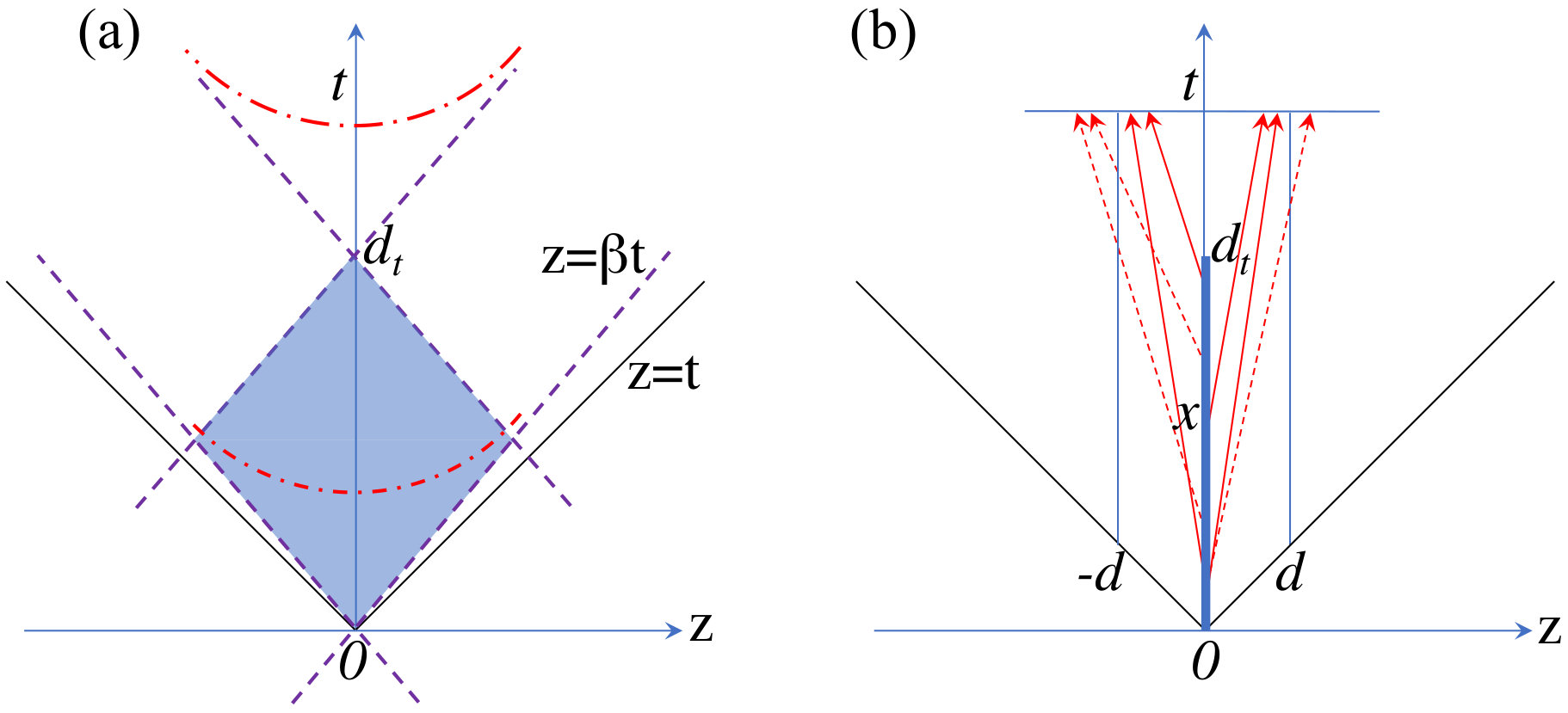 Figure 1
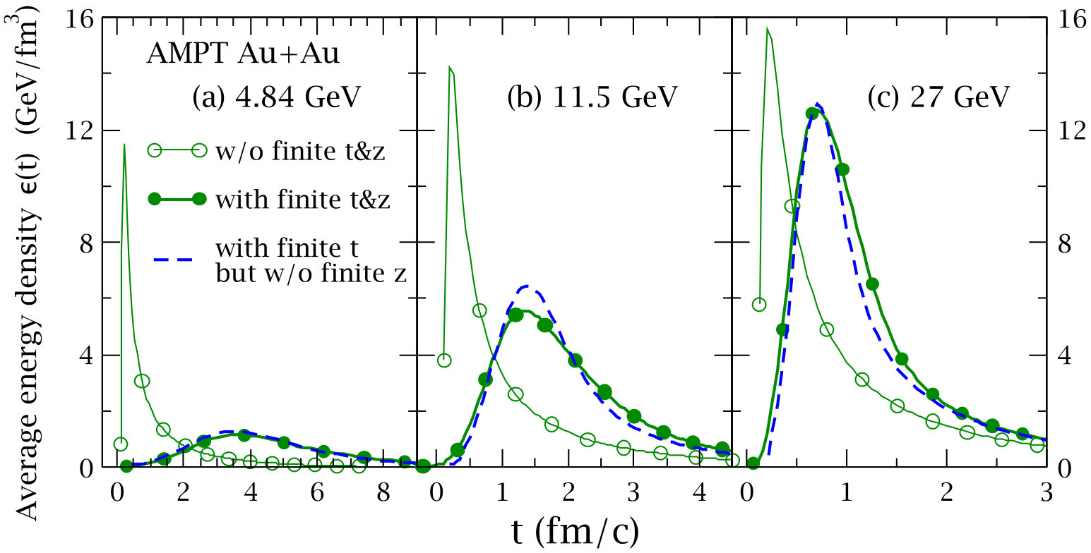 Figure 2
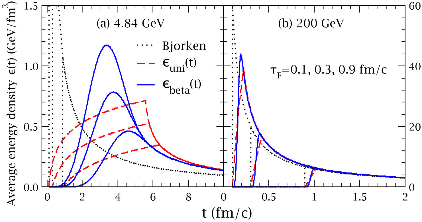 Figure 3
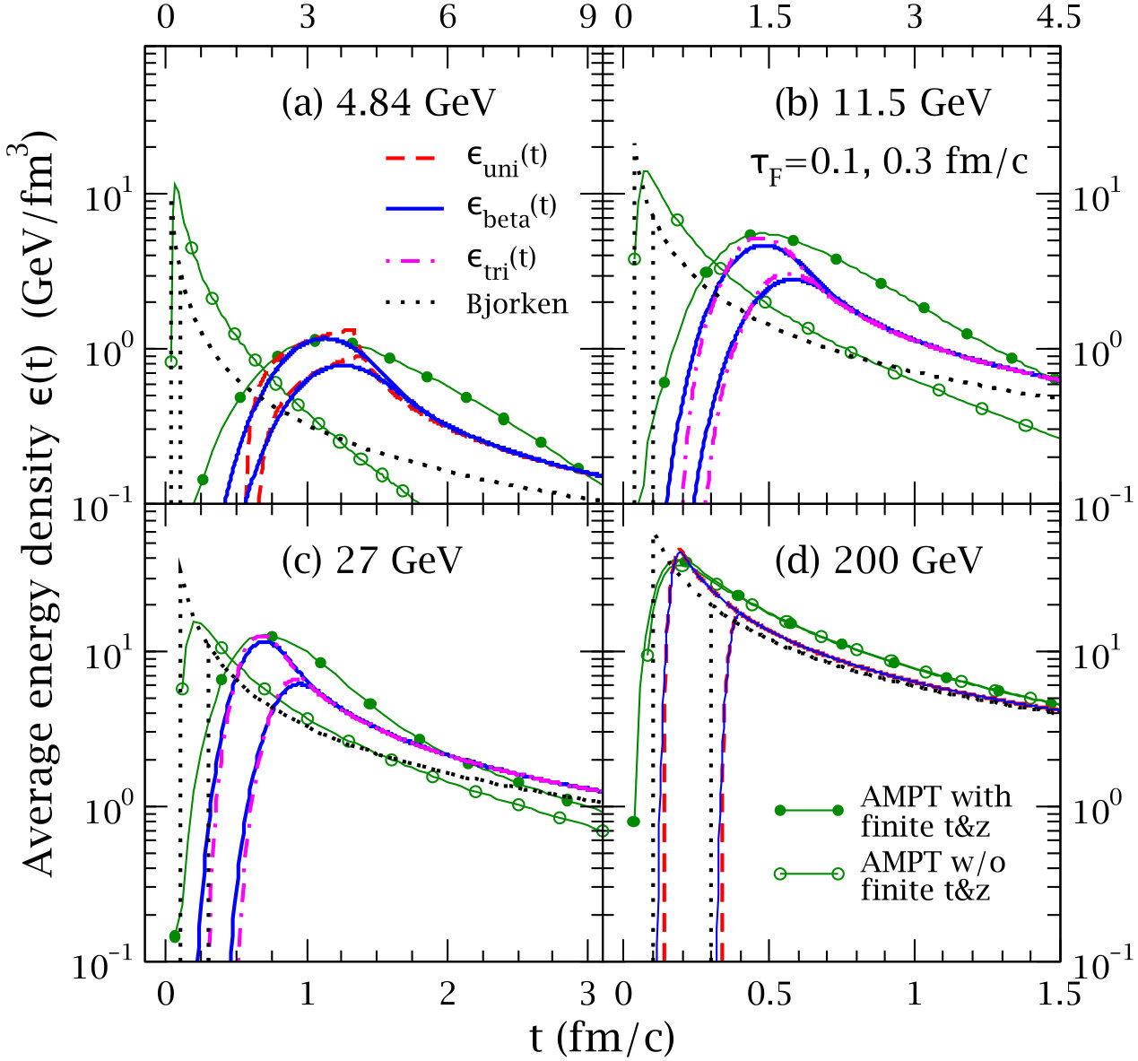 Figure 4
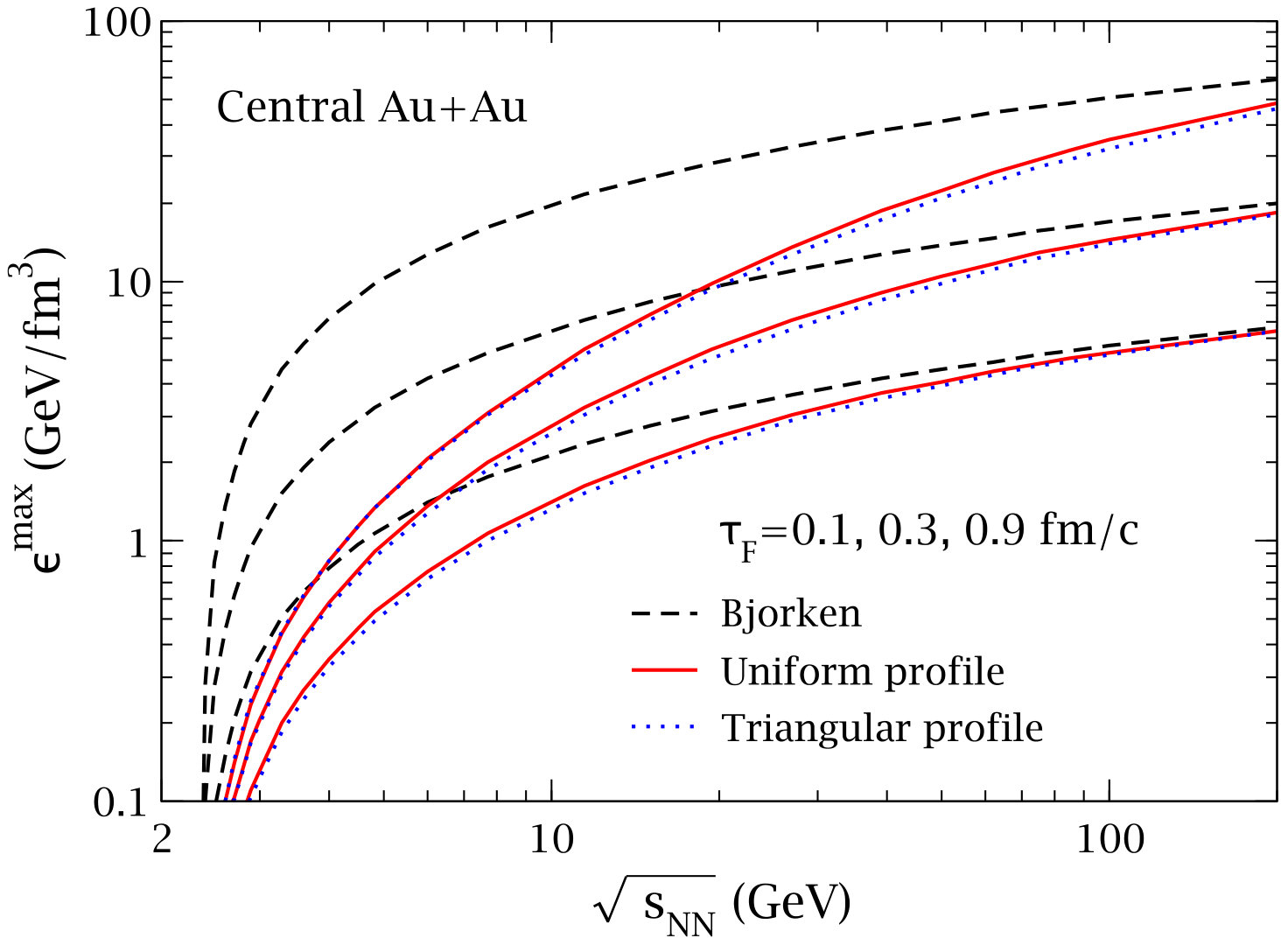 Figure 5
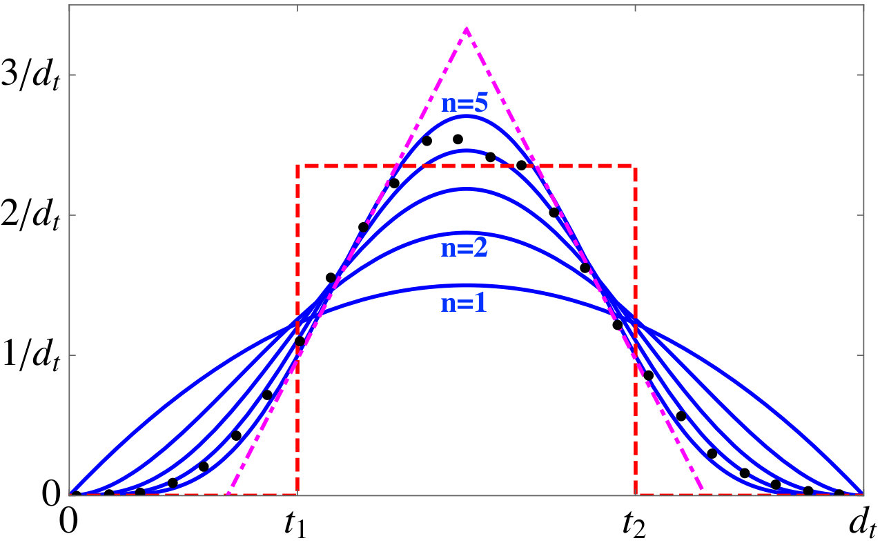 Figure 6
Peer Reviews
No public reviews on file for this paper yet. If you reviewed it on a platform where reviews are public (OpenReview, ICLR, NeurIPS, ICML), you can paste yours below so the community can read it here.
Videos
No videos yet. Explain this paper in a talk, walkthrough, or lecture? Add one.
Extension of the Bjorken energy density formula of the initial
state for relativistic heavy ion collisions
Zi-Wei Lin
Key Laboratory of Quarks and Lepton Physics (MOE) and Institute of Particle Physics, Central China Normal University, Wuhan 430079, China
Department of Physics, East Carolina University, Greenville, NC 27858, USA
Abstract
For relativistic heavy ion collisions, the Bjorken formula is very useful for estimating the initial energy density once an initial time is specified. However, it cannot be trusted at low energies, e.g. well below GeV for central Au+Au collisions, when is smaller than the finite time it takes for the two nuclei to cross each other. Here I extend the Bjorken formula by including the finite time duration of the initial energy production. Analytical solutions for the formed energy density in the central spacetime-rapidity region are derived for several time profiles. Compared to the Bjorken formula at low energies, the maximum energy density reached is much lower, increases much faster with the collision energy, and is much less sensitive to the uncertainty of the formation time, while the energy density time evolution is much longer. Comparisons with results from a multi-phase transport confirm the key features of these solutions. The effect of the finite longitudinal width of the initial energy production, which is neglected in the analytical results, is investigated with the transport model and shown to be small. This work thus provides a general model for the initial energy production of relativistic heavy ion collisions that is also valid at low energies.
pacs:
25.75.-q, 25.75.Ag, 25.75.Nq
I Introduction
Relativistic heavy ion collisions aim to create the quark-gluon plasma (QGP) and study its properties Adams:2005dq ; Adcox:2004mh . Therefore it is important to better understand the initial energy production, including the maximum value and time evolution of the energy density in the overlap volume. For low energies such as the Beam Energy Scan at the Relativistic Heavy Ion Collider, the relationship between the time evolution of the energy density or net-baryon density and the possible critical point of QCD becomes important Stephanov:2011pb ; Bialas:2016epd . The Bjorken formula Bjorken:1982qr is a very useful tool in estimating the initial energy density in the central rapidity region after the two nuclei pass each other:
[TABLE]
In the above, represents the full transverse area of the overlap volume, and is the rapidity density of the transverse energy at mid-rapidity (at an early time ), which is often approximated with the experimental value in the final state. Since the Bjorken energy density diverges as , a finite value is needed for the initial time Adcox:2004mh . Considering that the production of a particle takes a finite formation time , one can take the Bjorken formula at time to obtain the initial formed energy density.
A severe limitation of the above Bjorken energy density formula of the initial state results from the fact that it neglects the finite thickness of the colliding nuclei (along the beam direction ), which leads to a finite duration time, as well as a finite longitudinal width in , for the initial energy production. Using a hard-sphere model for the nucleus, it will take the following time for two nuclei of the same mass number to cross each other in a central collision in the center-of-mass frame Kajantie:1983ia :
[TABLE]
where is the projectile rapidity in the center-of-mass frame and is the nuclear radius. Therefore the Bjorken formula is only valid when the duration time (or crossing time) is much smaller than the formation time Adcox:2004mh . As an example, for fm/c, the Bjorken formula cannot be trusted for central Au+Au collisions well below GeV since fm/c there.
My goal of this study is to derive a Bjorken-like formula so that it is also valid at low energies where the Bjorken formula breaks down. I accomplish this by including the finite crossing time in the time profile of the initial energy production. I focus on the formed energy density, averaged over the full transverse overlap area, in the central spacetime-rapidity region () in the center-of-mass frame of central collisions of two identical nuclei.
II Method
Since the Bjorken formula Bjorken:1982qr is only valid at very high energies where the two incoming nuclei are highly Lorentz-contracted Adcox:2004mh , it essentially assumes that the initial energy production occurs at time . Then the quanta appear (i.e. are formed) after a certain proper time , as shown by the lower dot-dashed hyperbola in Fig. 1(a). This proper time can be viewed as a typical decay time of the color fields created from primary collisions of the two nuclei collection . Because of in the Bjorken ansatz, the quanta appearing at or are initially produced at time on the plane.
Once one considers the finite crossing time of the two nuclei, however, the initial energy production actually goes on throughout this period of time. Figure 1(a) shows a schematic picture, where the two nuclei come into contact at time [math] and pass each other at time Kajantie:1983ia . The two solid diagonal lines represent the light-cone boundaries (in natural units where the speed of light has been set to one), while each pair of the parallel dashed lines represents the boundaries of the trajectories of nucleons in an incoming nucleus that moves with speed . The shaded area, indicating the primary nucleon-nucleon collision region, shows that the initial energy production takes place over a finite amount of time. Again assuming a proper formation time , primary collisions at time [math] will then produce formed quanta on the lower hyperbola while primary collisions at time will produce formed quanta on the upper hyperbola as shown in Fig. 1(a). In addition, one sees that the initial energy is produced over a finite longitudinal width; for example, a particle initially produced at may propagate with a negative rapidity and later cross the plane.
To obtain analytical results for the central spacetime-rapidity region, I include the finite duration time in my formulation but neglect the finite longitudinal -width in the initial energy production. Figure 1(b) shows the simplified schematic picture for the region at , where the initial particles and energy are assumed to be produced over the crossing time but at . In order to obtain analytical results, I make minimal extensions to the Bjorken formula framework Bjorken:1982qr , thus I also neglect secondary particle interactions or the transverse expansion. The numerical results from a multi-phase transport (AMPT) model Lin:2004en , however, include the finite longitudinal width in , secondary parton scatterings, and the transverse expansion. In particular, I shall study with AMPT the effect of the finite longitudinal width in the initial energy production, which is neglected in the analytical formulation. Note that I only address the Bjorken energy density formula of the initial state Bjorken:1982qr ; Adcox:2004mh shown as Eq.(1), not the more general Bjorken model Bjorken:1982qr that also assumes local thermal equilibrium for the produced quanta in the initial state and then considers the subsequent hydrodynamic space-time evolution. Furthermore, since I only consider the central spacetime-rapidity region, I have written the time variable as instead of .
Let us write the production rate of the initial transverse energy rapidity density around at time as . Thus there could be particle productions at any time , while for or . With the picture of Fig. 1(b), I evaluate the energy density within a narrow region at time . For a particle produced at time to stay within this -region, its rapidity needs to satisfy
[TABLE]
at . Note that the right-hand-side above can always be made small with small-enough , so that does not depend on within this small -range. Therefore the average energy density in this region at time is
[TABLE]
From now on I shall study the formed energy density by assuming a finite formation time for the produced particles. A similar analysis gives the following average formed energy density at any time as
[TABLE]
As in the Bjorken formula, . However, an important feature of the above formula is that it applies to early times when the two nuclei are still crossing each other (i.e. ). Note that Eq.(5) above reduces to the Bjorken formula when one neglects the finite crossing time by taking . To proceed further, I will next take specific forms for the time profile of the initial energy production .
III Results
For simplicity, I first assume that the initial energy is produced uniformly from time to (with ):
[TABLE]
Note that one only needs the above assumption to apply at . Also, I have not related and to for the sake of generality. An illustration of this time profile is shown as the dashed curve in Fig. 2. Equation (5) then gives the following solution for the formed energy density:
[TABLE]
One can easily verify that, for and , this solution reduces to the Bjorken formula of Eq.(1).
Qualitatively, this energy density starts from 0 at time , grows smoothly to the following maximum value at time , and then decreases abruptly after the energy production stops:
[TABLE]
Compared to the maximum energy density given by the Bjorken formula, one has
[TABLE]
Therefore the value above is always smaller than the Bjorken initial energy density: at low energies where is small, while at high energies . Furthermore, as , the peak energy density grows as , much slower than the growth of the Bjorken formula. This means that, after taking into account the finite crossing time, the maximum energy density achieved will be much less sensitive to the uncertainty of , especially at lower energies where is bigger. In addition, Eq.(7) shows that the initial energy density at time later than is independent of . One will see next that these features are general and also apply to the other time profiles.
Due to the typical spherical shape of a nucleus, there will be few primary nucleon-nucleon interactions when the two nuclei barely touch or almost pass each other, while there will be many such interactions when the two nuclei fully overlap (around time ). I thus expect the time profile of the initial energy production to peak around time while diminish at time 0 and . Therefore I can choose the following time profile based on the probability density function of the beta distribution with equal shape parameters:
[TABLE]
In the above, power does not need to be an integer, and is the normalization factor with being the Beta function. This smooth beta profile reduces to a uniform profile when ; with an appropriate value of it can also well describe the transport model time profile, as shown in Fig. 2. I obtain the following solution for the formed energy density:
[TABLE]
above is the Appell hypergeometric function of two variables, and is the Gaussian hypergeometric function. One can verify that for the above solution reduces to Eq.(7) for & .
I now apply these solutions to central Au+Au collisions. The nuclear transverse area is taken as
[TABLE]
where . I take the mid-rapidity as the following data-based parameterization Adler:2004zn :
[TABLE]
where must be greater than in the unit of GeV. Also, I take for central collisions.
My results for central Au+Au collisions at GeV and 200 GeV are shown in Fig. 3 for different formation times & fm/c. Also shown are the results implied by the Bjorken formula: for (and for ). I have taken for the beta profile according to Fig. 2, and I take the naive choice of and for the uniform profile in Fig. 3. At 4.84 GeV, one sees that the time evolution of the energy density in either time profile has a much bigger width (e.g. full width at half maximum) than the Bjorken results, while the maximum energy density is much lower than the corresponding Bjorken value for the same . As expected, my maximum initial energy density changes by a much smaller factor of 2.1 (uniform profile) or 2.5 (beta profile) when changes from to fm/c; while the Bjorken initial energy density changes by a factor of 9. On the other hand, my results at 200 GeV are much closer to (although still different from) the Bjorken results; this is expected since the crossing time there ( fm/c) is very small. For both energies, my results approach the Bjorken results at late times.
Both the Bjorken formula and my method have neglected secondary particle interactions and the transverse expansion, which could affect the time evolution of the energy density. These dynamics can be described by transport models such as AMPT Lin:2004en or hydrodynamic models Shen:2012vn ; Oliinychenko:2014tqa . Now I compare my analytical solutions with results from the string melting AMPT model, which includes a conversion of excited strings into a parton matter, partonic scatterings, a quark coalescence for hadronization, and hadronic scatterings. For this study, the string melting AMPT model Lin:2004en has been improved by including the finite thickness of nuclei work , then I calculate the average local energy density (over the hard-sphere transverse area ) for partons at mid-spacetime-rapidity following the method of an earlier study Lin:2014tya . Circles in Fig. 2 represent the distribution of production time of partons within mid-spacetime-rapidity from AMPT for central ( fm) Au+Au collisions at GeV work . I thus take for the beta time profile, since this can reasonably describe the AMPT time profile. To get the same mean and standard deviation as the beta profile (for ), I set & for the uniform profile.
Figure 4 shows my results from different time profiles together with the Bjorken results at different energies. One sees from Figs. 4(a)&(d) that, unlike Figs. 3, results from the uniform and beta profiles here are quite close to each other once the uniform profile is set to the same mean and standard deviation as the beta profile. Curves with filled and open circles are respectively the AMPT results with and without the finite nuclear thickness. Note that each AMPT curve with finite thickness has been shifted a bit in time, so that it peaks at the same time as the corresponding beta profile for fm/c, in order to better compare their shapes. One sees that at the high energy of 200 GeV the AMPT results with and without the finite nuclear thickness are essentially the same; the Bjorken result and my analytical results are also very similar (especially after allowing shifts in time). This confirms that expectation that the finite nuclear thickness can be mostly neglected at high-enough energies. One also sees that the AMPT results are generally wider in time; partly because the parton proper formation time in AMPT is not set as a constant but is inversely proportional to the parent hadron transverse mass Lin:2004en ; I find that the parton formation time distribution at mid-spacetime-rapidity has a mean value of fm/c but has a long tail. The finite -width for the initial energy production, secondary parton scatterings, the transverse expansion, and the effective work done during the expansion Gyulassy:1983ub ; Ruuskanen:1984wv of the dense matter in AMPT can also cause differences from the analytical results. Overall, one sees that the AMPT results without considering the finite nuclear thickness are similar to the Bjorken results, while the AMPT results including the finite thickness are similar to my analytical results.
IV Discussions
One can also take a triangular time profile, as illustrated by the dot-dashed curve in Fig. 2, from time to with the peak at : for while for . One then obtains the following solution:
[TABLE]
This energy density increases smoothly to the following maximum value at a time within and then decreases smoothly with time:
[TABLE]
Figures 4(b)&(c) show that results from the beta and triangular profiles are almost identical in shape and close in magnitudes, after I set & for the triangular time profile to have the same mean and standard deviation as the beta profile for . An advantage of the triangular profile is that one has analytical expressions for its and the corresponding time.
Figure 5 compares , the maximum value of the average energy density at central spacetime-rapidity , in central Au+Au collisions from the Bjorken formula with that from my analytical extension, including the uniform and triangular time profiles that have analytical solutions for . My results from the uniform and triangular time profiles are quite close to each other after their and parameters are chosen so that each profile has the same mean and standard deviation as the beta profile for . One sees that the increase of the maximum energy density with the collision energy is much faster than the prediction from the Bjorken formula; this is consistent with Eq.(9), which shows that the Bjorken formula overestimates the maximum energy density more at lower energies. The overestimation of by the Bjorken formula is also more severe for smaller . At high energies, however, one sees that my results approach the Bjorken formula at the same . Note that these results are obtained using the parameterization in Eq.(13) Adler:2004zn , which precision should be improved at very low collision energies, e.g. when GeV.
Since my analytical method includes the finite time duration but neglects the finite -width for the initial energy production, further work may be warranted to include this effect analytically. Note that the finite width in is already included in one set of the AMPT results (curves with filled circles) shown in Fig. 4. Here I further demonstrate this effect numerically in Fig. 6. By modifying the AMPT model to include the finite width in but not the finite width in , I obtain the dashed curves in Fig. 6; they are quite close to the corresponding full AMPT result (filled circles) in both the peak magnitude and shape (with the width slightly smaller), while at low energies they are very different from the AMPT results that neglect both finite widths in and (open circles). These results suggest that the effect of the finite width in on my analytical results is rather small. Again note that, in order to better compare the shapes, each AMPT curve with finite thickness has been shifted a bit in time so that it peaks at the same value as the corresponding dashed curve. Similar to Fig. 5, one also sees in Fig. 6 that the increase of the maximum energy density with the collision energy is much faster after one includes the finite time duration of the initial energy production.
The analytical results of this study only address the energy density at spacetime-rapidity in the center-of-mass frame of the collision. Therefore the results for a realistic finite range of spacetime-rapidity, e.g. , would be somewhat different. Also, I have only addressed the energy density averaged over the full transverse overlap area . Note that the transverse overlap area at time before is smaller due to the partial overlap of the two nuclei. To average over this partial overlap area, one may replace in my solutions by for . This will enhance the energy density somewhat at early times. Also note that the finite duration of proper time in the initial energy production has been considered in hydrodynamic models Okai:2017ofp ; Shen:2017ruz , where an energy source term with a finite time duration can be introduced and my method can be applied to help describe the initial stage.
V Conclusions
I have extended the Bjorken formula by including a time profile for the initial energy production due to the finite nuclear thickness. By considering a simple uniform as well as more realistic time profiles, I have obtained analytical solutions of the formed energy density in the central spacetime-rapidity region. These solutions approach the Bjorken formula at high collision energies and/or at late times, but they are also valid at low energies where the Bjorken formula breaks down. I then apply the solutions to central Au+Au collisions in the energy range GeV. After taking into account the finite crossing time, at lower energies where the crossing time is bigger, the maximum energy density achieved is much less sensitive to the uncertainty of and increases much faster with the collision energy than the Bjorken formula. At low energies, the energy density reaches a much lower maximum value than the Bjorken energy density for the same formation time , but the width of the time evolution of energy density is much bigger. In addition, comparisons with the results from the string melting AMPT model confirm the key features of the analytical solutions. The AMPT results also suggest that the effect of the finite longitudinal width of the initial energy production on my analytical results is small. Therefore this extension provides a convenient tool to model the initial energy production in relativistic heavy ion collisions, especially at low energies.
Acknowledgments
I thank Miklos Gyulassy for careful reading of the manuscript and helpful comments. This work is supported in part by National Natural Science Foundation of China grant No. 11628508.
The reference list from the paper itself. Each links out to its DOI / PubMed record.
- 1(1) J. Adams et al. [STAR Collaboration], Nucl. Phys. A 757 , 102 (2005).
- 2(2) K. Adcox et al. [PHENIX Collaboration], Nucl. Phys. A 757 , 184 (2005).
- 3(3) M. A. Stephanov, Phys. Rev. Lett. 107 , 052301 (2011).
- 4(4) A. Bialas, A. Bzdak and V. Koch, Acta Phys. Polon. B 49 , 103 (2018).
- 5(5) J. D. Bjorken, Phys. Rev. D 27 , 140 (1983).
- 6(6) K. Kajantie, R. Raitio and P. V. Ruuskanen, Nucl. Phys. B 222 , 152 (1983).
- 7(7) G. Gatoff, A. K. Kerman and T. Matsui, Phys. Rev. D 36 , 114 (1987); A. Bialas, W. Czyz, A. Dyrek and W. Florkowski, Nucl. Phys. B 296 , 611 (1988); H. T. Elze and U. W. Heinz, Phys. Rept. 183 , 81 (1989); A. Kovner, L. D. Mc Lerran and H. Weigert, Phys. Rev. D 52 , 6231 (1995); G. C. Nayak and V. Ravishankar, ibid. 55 , 6877 (1997) & Phys. Rev. C 58 , 356 (1998); D. D. Dietrich, G. C. Nayak and W. Greiner, Phys. Rev. D 64 , 074006 (2001); F. Gelis, K. Kajantie and T. Lappi, Phys
- 8(8) Z. W. Lin, C. M. Ko, B. A. Li, B. Zhang and S. Pal, Phys. Rev. C 72 , 064901 (2005).