Boundary classification and 2-ended splittings of groups with isolated flats
Matthew Haulmark

TL;DR
This paper classifies 1-dimensional boundaries of groups with isolated flats acting on CAT(0) spaces, showing they are homeomorphic to well-known fractals or circles unless the group splits over a virtually cyclic subgroup.
Contribution
It generalizes previous theorems by Kapovich-Kleiner and Bowditch, providing a comprehensive classification of boundaries and their relation to group splittings in this setting.
Findings
Boundaries are homeomorphic to circle, Sierpinski carpet, or Menger curve under certain conditions.
Existence of local cut points implies the group splits over a 2-ended subgroup.
The classification extends previous results to a broader class of groups with isolated flats.
Abstract
In this paper we provide a classification theorem for 1-dimensional boundaries of groups with isolated flats. Given a group acting geometrically on a space with isolated flats and 1-dimensional boundary, we show that if does not split over a virtually cyclic subgroup, then is homeomorphic to a circle, a Sierpinski carpet, or a Menger curve. This theorem generalizes a theorem of Kapovich-Kleiner, and resolves a question due to Kim Ruane. We also study the relationship between local cut points in and splittings of over -ended subgroups. In particular, we generalize a theorem of Bowditch by showing that the existence of a local point in implies that splits over a -ended subgroup.
Click any figure to enlarge with its caption.
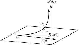 Figure 1
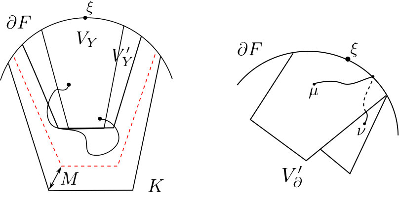 Figure 2
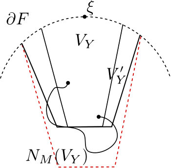 Figure 3
Peer Reviews
No public reviews on file for this paper yet. If you reviewed it on a platform where reviews are public (OpenReview, ICLR, NeurIPS, ICML), you can paste yours below so the community can read it here.
Videos
No videos yet. Explain this paper in a talk, walkthrough, or lecture? Add one.
Boundary classification and 2-ended splittings of groups with isolated flats
Matthew Haulmark
Department of Mathematics
1326 Stevenson Center
Vanderbilt University
Nashville, TN 37240 USA
Abstract.
In this paper we provide a classification theorem for 1-dimensional boundaries of groups with isolated flats. Given a group acting geometrically on a space with isolated flats and 1-dimensional boundary, we show that if does not split over a virtually cyclic subgroup, then is homeomorphic to a circle, a Sierpinski carpet, or a Menger curve. This theorem generalizes a theorem of Kapovich-Kleiner, and resolves a question due to Kim Ruane.
We also study the relationship between local cut points in and splittings of over -ended subgroups. In particular, we generalize a theorem of Bowditch by showing that the existence of a local point in implies that splits over a -ended subgroup.
Key words and phrases:
, Isolated Flats, Group Boundaries, JSJ Decompositions, Splittings, Ends of Spaces
1. Introduction
When a group acts discretely on a geometric space , we can often compactify by attaching a “boundary at infinity” to . In the presence of non-positive curvature, has an induced action by homeomorphisms on the boundary. There are strong connections between the topological properties of and the algebraic properties of . A natural question posed by Kapovich and Kleiner [28] is: which topological spaces occur as boundaries of groups?
In [28] Kapovich and Kleiner prove a classification theorem for boundaries of one-ended hyperbolic groups. They show that if the boundary is -dimensional and the group does not split over a virtually cyclic subgroup then the boundary of the group is either a circle, a Sierpinski carpet, or a Menger curve.
Problem 1.1** (K. Ruane).**
Can the Kapovich-Kleiner result be extended to some natural family of groups?
Kapovich and Kleiner’s result relies heavily on JSJ results due to Bowditch [11]. Bowditch’s results relate the existence of local cut points in the boundary to the existence of cut pairs, which is further related to two-ended splittings of the group. For groups Papasoglu and Swenson [32] extend the connection between cut pairs and two-ended splittings, but leave the issue of local cut points completely unresolved.
In this article we resolve this issue for groups acting geometrically (i.e. properly, cocompactly, and by isometries) on a space with isolated flats (see [25]) and obtain the following result:
Theorem 1.2** (Main Theorem).**
Let be a group acting geometrically on a space with isolated flats. Assume is one-dimensional. If does not split over a virtually cyclic subgroup then one of the following holds:
- (1)
* is a circle* 2. (2)
* is a Sierpinski carpet* 3. (3)
* is a Menger curve.*
A key tool used by Kapovich and Kleiner is the topological characterization of the Menger curve due to R.D. Anderson [1, 2]. Anderson’s theorem states that a compact metric space is a Menger curve provided: M is -dimensional, M is connected, M is locally connected, M has no local cut points, and no non-empty open subset of M is planar. We note that if the last condition is replaced with “M is planar,” then we have the topological characterization of the Sierpinski carpet (see Whyburn [36]).
Prior to Kapovich and Kleiner’s theorem [28], results of Bestvina and Mess [6], Swarup [33], and Bowditch [8] had shown that the boundary of a one-ended hyperbolic group is connected and locally connected. The planarity issue is easily dealt with using the dynamics of the action of the group on its boundary, leaving only the local cut point issue. However, Bowditch has shown [11] that if is not homeomorphic to a circle, then has a local cut point if and only if splits over a two-ended subgroup.
We follow a similar outline to prove Theorem 1.2. The question of which groups with isolated flats have locally connected boundary has been completely determined by Hruska and Ruane [27]. So we will begin by assuming, for now, that is locally connected. In the isolated flats setting the planarity is again easily dealt with using an argument similar to that of Kapovich and Kleiner, leaving only the local cut point issue. So in order to complete the proof of Theorem 1.2, the remaining difficulty is understanding the connection between local cut points in and splittings of .
We prove the following splitting theorem which is independent of the dimension of and thus more general than is required for the proof of Theorem 1.2:
Theorem 1.3**.**
Let be a group acting geometrically on a space with isolated flats. Suppose is locally connected and not homeomorphic to . If does not split over a virtually cyclic subgroup, then has no local cut points.
Techniques developed by the author for the proof of Theorem 1.3 have already been used by Hruska and Ruane [27] in the proof of their local connectedness theorem. In the special case when the boundary is one-dimensional Hruska and Ruane’s [27] theorem shows reduces to the statement that is locally connected if does not split over a two-ended subgroup (see Theorem 2.3). So, we obtain a simplified version of Theorem 1.3, which is used in the proof of Theorem 1.2.
Corollary 1.4**.**
Let be a one-ended group acting geometrically on a space with isolated flats and assume that is 1-dimensional and not homeomorphic to . If does not split over a virtually cyclic subgroup, then has no local cut points.
Theorem 1.3 fills a gap in the JSJ theory literature on groups and most of this paper is spent on the proof. We mention that the significance of this gap in the literature has also been observed by Świątkowski [34].
In [11] Bowditch studied local cut points in boundaries of hyperbolic groups and their relation to so called JSJ-splittings. As mentioned above, Bowditch showed that for a one-ended hyperbolic group which is not cocompact Fuchsian the existence of a local cut point is equivalent to a splitting of over a -ended subgroup. Generalizations of Bowditch’s results have been studied by Papasoglu-Swenson [31] [32], and Groff [18] for and relatively hyperbolic groups, respectively.
Groups with isolated flats have a natural relatively hyperbolic structure [25], and there is a strong relationship between and the Bowditch boundary . Analogous to the limit set of a Kleinian group, the Bowditch boundary was introduced by Bowditch [10] and used to study splittings of hyperbolic groups. In general may have infintely many global cut points. In fact, the global cut point structure of is key to a general theory of splittings [9].
Using cut pairs instead of local cut points Groff [18] obtains a partial extension of Bowditch’s JSJ tree construction [11] for relatively hyperbolic groups, and Guralnik [22] observed that in the special case that the relative boundary has no global cut points, then many of Bowditch’s results [11] about the valence of local cut points in the boundary of a hyperbolic group translate directly to the relatively hyperbolic setting. Their results were subsequently used by Groves and Manning [20] to show that if has no global cut points and all the peripheral subgroups are one-ended, then the existence of a local cut point in is equivalent to the existence of a splitting of relative to over a non-parabolic -ended subgroup. The relative boundary (or Bowditch boundary) is different from the boundary mentioned above.
In [23] the author investigates local cut points in and provides a splitting theorem for relatively hyperbolic groups without making any assumptions about global cut points. Namely, he shows that under some very modest conditions on the peripheral subgroups, the existence of a non-parabolic local cut point in implies that splits over a -ended subgroup (see Theorem 2.5). Because of the close relationship between and , this splitting theorem will be used in Section 6 to show that the existence of a local cut point of which is not in the boundary of a flat implies that splits over a -ended subgroup.
We conclude the paper by discussing applications of Theorem 1.2. In particular, in Section 10 we discuss groups with Menger curve boundary and in Section 9 we generalize the work of Świątkowski [34] to obtain the following result:
Theorem 1.5**.**
Let be a Coxeter system such that has isolated flats. Assume that the nerve of the system is planar, distinct from simplex, and distinct from a triangulation of . If the labeled nerve of is distinct from a labeled wheel and inseparable, then is homeomorphic to the Sierpinski carpet.
Definitions of the terms used in Theorem 1.5 can be found in Section 9.
In [17] Davis and Okun show that if is a Coxeter group whose nerve is planar, then acts properly on a -manifold. Consequently, Theorem 1.5 is in line with the following extension of a conjecture due to Kapovich and Kleiner [28]:
Conjecture 1.6**.**
Let be a group with isolated flats and Sierpinski carpet boundary. Then acts properly on a contractible -manifold.
1.1. Methods of Proof
The strong connection between and the boundary is given by Hung Cong Tran [35]. For spaces with isolated flats Tran’s result implies that is the quotient space obtained from by identifying points which are in the boundary of the same flat. Using basic decomposition theory (see Section 6.1), we are able to show that if there exists a local cut point that is not in the boundary of a flat, then it must push forward under this quotient map to a local cut point of . This allows us to apply Theorem 2.5 mentioned above, and prove that the existence of a local cut point that is not in the boundary of a flat implies the existence of a -ended splitting (see Proposition 6.1).
Assuming that our group does not split over a two ended group, we are left with the remaining question: Can a point which lies in the boundary of a flat be a local cut point? Much of this paper is spent answering that question in the negative when is locally connected. Let be a space which has isolated flats with respect to and let be an -dimensional flat in , then it can be shown that has a finite index subgroup isomorphic to . In Section 3 we show that acts properly and cocompactly on . This is done by means of a relation on , which uses orthogonal rays to associate points in with points in the boundary. In Sections 4 and 5 we assume that is locally connected and show that we may put an -equivariant metric on . Then in Section 7 we use the properties of this action to deduce that a point in the boundary of a flat cannot be a local cut point. This combined with Proposition 6.1 allow us to obtain Theorem 1.3.
Once we have completed the proof of Theorem 1.3 we are ready to prove Theorem 1.2. This is accomplished in Section 8 with an argument inspired by Kapovich and Kleiner [28]. Using the dynamics of the action of on the boundary we show that if contains a non-planar graph , then every open subset of must contain a homeomorphic copy of . This will be enough to complete the proof.
1.2. Acknowledgments
First and foremost, I would like to thank my advisor Chris Hruska for his guidance throughout this project. Second, I would like to thank the rest of UWM topology group Craig Guilbault, Ric Ancel, and Boris Okun for suggesting simplifications for some my arguments. I would also, like to thank Kim Ruane, Jason Manning, and Kevin Schreve for helpful conversations.
2. Preliminaries
2.1. The Bordification of a Space
Throughout this paper we will assume that is a proper metric space, unless otherwise stated. We refer the reader to [12] for definitions and basic results about spaces.
The boundary of , denoted , is the set of equivalence classes of geodesic rays. Where two rays are equivalent if there exists a constant such that d\big{(}c_{1}(t),c_{2}(t)\big{)}\leq D for all . The bordification of is the set .
The bordification comes equipped with a natural topology called the cone topology, where one considers rays based at some fixed point. A basis for the cone topology consists of open balls in together with “neighborhoods of points at infinity.” Given a geodesic ray and positive numbers , , define
[TABLE]
Where is the orthogonal projection onto the closed ball \overline{B}\big{(}c(0),t\big{)}. For fixed and the sets form a neighborhood base at infinity about . Intuitively, this means that two points in will be close if they are represented by rays which are close at for large values of . We will denote by the set .
2.2. The Bowditch Boundary and Splittings
Let be a group and a collection of infinite subgroups which is closed under conjugation, called peripheral subgroups.
We say that is if admits a proper isometric action on a proper -hyperbolic space such that:
- (i)
is the set of all maximal parabolic subgroups 2. (ii)
There exists a -invariant system of disjoint open horoballs based at the parabolic points of , such that if is the union of these horoballs, then acts cocompactly on .
The Bowditch boundary of is defined to be the boundary of the space . If is relatively hyperbolic and acts geometrically on a space there is a close relationship between the and the visual boundary .
Theorem 2.1** (Tran).**
* is -equivariantly homeomorphic to the quotient of obtained by identifying points which are in the boundary of the same flat.*
A splitting of a group over a given class of subgroups is a finite graph of groups of , where each edge group belongs to the given class. A splitting is called trivial if there exists a vertex group equal to . Assume that is hyperbolic relative to a collection . A peripheral splitting of is a finite bipartite graph of groups representation of , where is the set of conjugacy classes of vertex groups of one color of the partition called peripheral vertices. Nonperipheral vertex groups will be referred to as components. This terminology stems from the correspondence between the cut point tree of and the peripheral splitting of , where elements of correspond to cut point vertices and the components correspond to components of the boundary (i.e. equivalence classes of points not separated by cut points).
A peripheral splitting is a refinement of another peripheral splitting if can be obtained from via a finite sequence of foldings that preserve the vertex coloring. In [9] Bowditch proved the following accessibility result:
Theorem 2.2**.**
Suppose that is relatively hyperbolic and that is connected. Then admits a (possibly trivial) peripheral splitting which is maximal in the sense that it is not a refinement of any other peripheral splitting.
2.3. Isolated Flats
Here we introduce basic definitions and pertinent results regarding spaces with isolated flats. We refer the reader to [25] for a more detailed account. Let be a space with acting geometrically on . A k-flat in is an isometrically embedded copy of Euclidean space, . A -flat will also be referred to as a line and a -flat may be referred to as a flat plane.
The space is said to have isolated flats if there is a -invariant collection of flats, , of dimension 2 or greater and such that the following hold:
- (i)
(capturing condition) There exists a constant such that each flat in lies in the -tubular neighborhood of some 2. (ii)
(isolating condition) For every there exists such that for any two distinct we have \operatorname{diam}\big{(}\mathcal{N}_{\rho}(F)\cap\mathcal{N}_{\rho}(F^{\prime})\big{)}<\kappa(\rho)
Hruska and Kleiner have shown in [25] that if is a group acting geometrically on a space with isolated flats, then is hyperbolic relative to a collection of virtually abelian subgroups of rank at least 2 (Theorem 1.2.1 of [25]). Hruska and Kleiner have also shown that for isolated flats is an invariant of the group up to quasi-isometry (Theorem 1.2.2 of [25]). The following recent result concerning groups with isolated flats is due to Hruska and Ruane [27], and is particularly relevant to this project:
Theorem 2.3** (Hruska-Ruane).**
Let be a one-ended group acting geometrically on a space with isolated flats. Let be the maximal peripheral splitting of . Then each vertex group of acts geometrically on a space with locally connected boundary.
Furthermore is locally connected if and only if the following condition holds: Each edge group of has finite index in the adjacent peripheral vertex group.
In the case where is -dimensional we have the following corollary:
Corollary 2.4**.**
Assume is acting geometrically on a space with isolated flats, and assume is -dimensional. Then is locally connected if and only if does not have a peripheral splitting over a -ended subgroup.
Remark**.**
As “no splitting over a two-ended subgroup” is a hypothesis in both Theorem 1.2 and Theorem 1.3, we may assume that is locally connected when required. Also, notice that for the proof of Theorem 1.2 we are concerned with 1-dimensional boundaries, so in that case the dimension of the flats we are interested in is 2. However, for many of the result we will not need to make any assumption about the dimension of flats.
2.4. Local Cut Points
Recall that a continuum is a non-empty, connected, compact, metric space, and let be such a space. A cut point of is a point such that is disconnected. A point is a local cut point if is a cut point or has more than one end. A detailed discussion of ends of spaces can be found in Section 3 of [21]. In this paper we are often interested in whether a given point is a local cut point or not. Thus we remark that saying a point is a local cut point is equivalent to saying that there exists a neighborhood of such that for every neighborhood of with , there exist points which cannot be connected inside , i.e. and are not contained in the same connected subset of . In Section 7 we will be interested in showing that a point cannot be a local cut point, so it is worth noting the negation of the above. In other words, to check that is not a local cut point it suffices to show that given a neighborhood of there exists a neighborhood with and connected.
In his study of JSJ splittings of hyperbolic groups Bowditch investigated the local cut point structure of the boundary. In that setting Bowditch shows that the existence of a local cut point implies that group splits over a 2-ended subgroup. In [23] the author studies local cut points in the relative boundary (or Bowditch Boundary) and has generalized Bowditch’s result to show:
Theorem 2.5**.**
Let be a relatively hyperbolic group and suppose each is finitely presented, one- or two-ended, and contains no infinite torsion subgroup. Assume that is connected and not homeomorphic to a circle. If contains a non-parabolic local cut point, then splits over a -ended subgroup.
The majority of this paper is concerned with determining the existence or non-existence of local cut points . Theorem 2.5 will be used in Section 6 to show that the existence of a local cut point which is not in the boundary of a flat implies the existence of a splitting over 2-ended subgroup.
2.5. Limit Sets
We will need a few basic results about limit sets sporadically through this paper, consequently, we conclude the preliminary section with a terse discussion of limit sets. In this section will be a space and some group of isometries of .
Recall, that a for a sequence we write if for some . It is clear that if for some , then for any . The limit set, , of is the subset of consisting of all such limits. The set is a closed and -invariant. Given that the action of is geometric we have the following:
Lemma 2.6**.**
**
We leave the proof of this result as an exercise.
A subset of is said to be minimal if is closed, non-empty, -invariant, and does not properly contain a closed -invariant subset. A useful fact about minimal sets is that is minimal if and only if is dense in for every . The action of on is called minimal if is minimal.
3. A Proper and Cocompact Action on
Let be a space with isolated flats and let be a flat in . Set . In this section we a follow a strategy similar to that of Bowditch in Lemma 6.3 of [10] to show that acts properly and cocompactly on . The key observation made by Bowditch is as follows:
Lemma 3.1**.**
Let be a group acting on topological spaces and . Define the action of on to be the diagonal action and let . If is -invariant and the projections and from onto the factors are both proper and surjective, then the following are equivalent:
- (a)
* acts properly and cocompactly on * 2. (b)
* acts properly and cocompactly on * 3. (c)
* acts properly and cocompactly on *
Set . Define be the set of all geodesic rays orthogonal to . Recall that a geodsic ray is orthogonal to a convex set if for every and for any the Alexandrov angle, \angle_{r(0)}\big{(}r(t),y\big{)}, is greater than or equal to . It is well known that acts cocompactly on (see [25] Lemma 3.1.2). Let be the diameter of the fundamental domain of this action. We define \mathcal{R}=\big{\{}(x,q)\big{|}\hskip 2.84526ptq\in\perp(F)\hskip 2.84526pt\text{with}\hskip 2.84526ptd\big{(}x,q(0)\big{)}\leq A\big{\}}. Unless otherwise stated, we will assume that our base point is in the flat .
We want that satisfies the hypotheses of Lemma 3.1, with the roles of and played by and . We begin with the following observation:
Lemma 3.2**.**
* is -invariant.*
Proof.
acts on by isometries, so if and then d\big{(}h.x,h.q(0)\big{)}<A. If is the orthogonal projection onto , then by d\big{(}h.q(t),h.q(0)\big{)}=d\big{(}q(t),q(0)\big{)} and the uniqueness of the projection point (see [12] Proposition II.2.4) we must have that \pi_{F}\big{(}h.q(t)\big{)}=h.\pi_{F}\big{(}q(t)\big{)} for every . ∎
To continue our study of , we require the following useful lemma, which allows one to construct a new orthogonal ray from a sequence of orthogonal rays with convergent base points. The proof relies on a standard diagonal argument and will not be presented here; however, it is not dissimilar to the proof presented in Lemma 5.31 of [12].
Lemma 3.3**.**
If is a separable metric space, is proper metric space, , and a compact subset of , then any sequence of isometric embeddings, , with has a subsequence which converges point-wise to an isometric embedding .
Next, we check that projects surjectively onto the factors and .
Lemma 3.4**.**
Let . If is a ray representing , then there exists a geodesic ray asymptotic to .
Proof.
Let and for all . Our first claim is that the sequence is bounded as . Assume not, then . By Corollary 7 of [26] there exists some constant such that d\big{(}x_{0},[x_{n},y_{n}]\big{)}<M for all . Then by the triangle inequality and the definition of as the orthogonal projection we have that . Then converges in and we may apply Lemma 3.3 to construct the orthogonal ray . ∎
Corollary 3.5**.**
The projections and are surjective.
Proof.
The surjectivity of is immediate. For we need only that each point in the flat is within a bounded distance of an element of . Let be the constant used in the definition of above. We know from the previous lemma that there exists some . The result follows as and is -dense. ∎
In order to check the properness of the projections, we need to know that as a sequence of orthogonal rays moves the corresponding sequence of asymptotic rays based at travel within a bounded distance of the points \big{(}r_{n}(0)\big{)}. We provide a quasiconvexity result below, which is a corollary of the following theorem presented by Hruska and Ruane in 4.14 of Theorem [27].
Theorem 3.6**.**
Let be a space with isolated flats with respect to . There exists a constant such that the following hold:
- (1)
Given two flats with the shortest length geodesic from to , we have that is -quasiconvex in . 2. (2)
Given a point and a flat , with the shortest path from to , then is -quasiconvex in .
Lemma 3.7**.**
Let and then there exists a constant such that is -quasiconvex in .
Proof.
The proof follows from the Theorem 3.6 by passing to the limit as of the geodesic segments \big{[}q(n),q(0)\big{]}. ∎
To prove properness we will also need to know that convergence of orthogonal rays in the space corresponds to convergence of points in .
Lemma 3.8**.**
If ) is a sequence of rays in which converge pointwise to an element of , then the corresponding points at infinity converge in the topology on .
Proof.
Let be the base point for the cone topology on and let be limit ray. For each ray there exists a an asymptotic ray based at (see [12] Chapter II.8 Proposition 8.2). Define D=d\big{(}x_{0},r(0)\big{)}, then d\big{(}r_{n}(t),c_{n}(t)\big{)}\leq D for every . Thus we may apply Lemma 3.3 with to find the limiting based ray . Then is asymptotic to . The claim is that in the cone topology. Fix and let . Then U(c,s,\epsilon)=\bigl{\{}\,{c^{\prime}\in\partial_{x_{0}}X}\bigm{|}{d\big{(}c^{\prime}(s),c(s)\big{)}<\epsilon}\,\bigr{\}} is a basic neighborhood of . As pointwise we have that there exists d\big{(}c_{m}(s),c(s)\big{)}<\epsilon for every . Thus we have the claim. ∎
We now wish to prove that the projections and are proper. In order to do so we will need several lemmas concerning the relationship between base points of orthogonal rays and the based rays which represent them in the boundary (See Figure 1 for an intuitive picture).
Lemma 3.9**.**
There is a constant such that for any , d\big{(}\omega(0),c(t)\big{)}<M where is the ray based at representing and t=d\big{(}x_{0},\omega(0)\big{)}.
Proof.
Let be the geodesic with and . By Corollary 3.7 there exists a constant such that is contained within the -tubular neighborhood of . This implies that there exists an , , and with d\big{(}c(s),x\big{)}\leq L and d\big{(}c(s),y\big{)}\leq L. By orthogonal projection we know that d\big{(}x,\omega(0)\big{)}\leq 2L, which implies that d\big{(}c(s),\omega(0)\big{)}\leq 3L. Because, and are geodesics the triangle inequality gives us that t\in\big{[}s-3L,s+3L\big{]}. Thus setting we are done. ∎
Lemma 3.10**.**
Suppose and let be the constant found in Lemma 3.9. There is a constant such that for any and the following holds: if with and is the ray based at representing , then .
Proof.
Let be the geodesic with and . If is the constant from Lemma 3.9, then we know that d\big{(}\beta(a),c(a)\big{)}\leq M. So, if we are done.
Assume that . Then by convexity d\big{(}c(n),\beta(n)\big{)}\leq M and d\big{(}\beta(n),\eta(n)\big{)}\leq\epsilon, which implies that d\big{(}c(n),\eta(n)\big{)}\leq M+\epsilon.
If , then . By hypothesis , which implies that d\big{(}\beta(a),\eta(n)\big{)}<\epsilon. So, d\big{(}c(a),\eta(n)\big{)}\leq M+\epsilon, but and are geodesics so we have that d\big{(}c(n),\eta(n)\big{)}\leq 2(M+\epsilon). Set . ∎
Lemma 3.11**.**
Let be compact. The set of all points with d\big{(}x,w(0)\big{)}\leq A for some is bounded.
Proof.
Assume not, then there exists a sequence in with for every such that as for some . For every let be the ray based at the base point and asymptotic to .
Recall that for any the sets form a neighborhood base at . Fix . Then implies that for any we have lies in for all but finitely many . Lemma 3.10 then gives us that for any we have lies in for all but finitely many , which by Lemma 3.8 implies that , a contradiction. ∎
Lemma 3.12**.**
The projections and are proper.
Proof.
Let be compact. We want that is compact. Let ) be a sequence of rays in with base points in . As is compact using Lemma 3.3 we know that the sequence has a subsequence which converges to a ray based in . Set , , and let be some fixed point in . We know that and that the function is upper semi-continuous for all (see [12] Proposition II.3.3(1)), thus must be a ray orthogonal to . By Lemma 3.8 we have that the sequence of points at infinity converges, which implies that is compact.
Now, let be a compact subset of and the set of all points with d\big{(}x,w(0)\big{)}\leq A for some . We need that is compact. By Lemma 3.11 the set is bounded. We only need that is closed.
Assume that is a limit point of . Then there exists a sequence of points in which converge to , and there exists a sequence of rays in with d\big{(}c_{i},w_{i}(0)\big{)}\leq A and for every . The sequence \big{(}w_{i}(0)\big{)}_{i=0}^{\infty} converges in , so by a diagonal argument we have that converges to a ray . Lemma 3.8 and compactness of give that . It is now easy to see that d\big{(}c,w(0)\big{)}\leq A.∎
Combining the previous results we may apply Lemma 3.1 to conclude:
Theorem 3.13**.**
Let . Then acts properly and cocompactly on .
As mentioned above in Lemma 3.1.2 of [25] Hruska and Kleiner showed that acts cocompactly on . The Beiberbach theorem then gives that contains a subgroup of finite index isomorphic to , where is the rank of the flat .
We then obtain the following corollary:
Corollary 3.14**.**
The subgroup acts properly and cocompactly on .
4. Additional Properties of
Throughout this section we will assume that is locally connected. Let be the collection of connected components of . The goal of this section is to show that has finitely many orbits and that the stabilizer of each has a finite index subgroup isomorphic to , where is the dimension of the flat. This fact will play a crucial role in Sections 5 and 7.
Let be a closed convex subset of a metric space , and let be any subgroup of . We say is -periodic if acts cocompactly on . As in the previous section let be a finite index subgroup isomorphic to , where is the dimension of . We begin with two results concerning the -periodicity of elements of that will be needed to prove the main result of this section.
4.1. H-periodicity
Lemma 4.1**.**
The collection is locally finite, i.e only finitely many intersect any compact set
Proof.
This simply follows from the local connectedness of . Assume that is not locally finite. Then there exists such that meets infinitely many elements of . We may then find a sequence of points from distinct elements of which meet . This sequence must converge to a point in . Thus any neighborhood of meets infinitely many members of . is an open subset of a locally connected space and thus must be locally connected, a contradiction. ∎
Lemma 4.2**.**
Let be as above. Then we have the following:
- (i)
The elements of lie in only finitely many -orbits. 2. (ii)
Each is -periodic, i.e acts cocompactly on .
Proof.
From Lemma 4.1 we know that is locally finite, and we saw in Corollary 3.14 that acts properly and cocompactly on on . We may now follow word for word the proof of Lemma 3.1.2 of [25].∎
4.2. Full Rank Components
Lemma 4.3**.**
Assume we have a sequence of rays in with base points, , converging to a point in , then the sequence \big{(}r_{i}(\infty)\big{)} converges to in .
Proof.
By Corollary 3.7 each point is represented by based rays that stay within the -neighborhood of im. Thus if , then for any all but finitely many members of the sequence \big{(}r_{i}(0)\big{)} are inside , which implies that for any all but finitely many lie in .∎
Corollary 4.4**.**
Every point in is a limit point of points in .
Proof.
Let be in the boundary of a and a based ray representing . Then by Corollary 3.5 for each there is an such that d\big{(}c(n),r_{n}(0)\big{)}<A. So, the sequence converges to and we may apply the preceding lemma. ∎
The proof of the following lemma essentially amounts to checking Bestvina’s nullity condition [5] for the action of on .
Lemma 4.5**.**
If then elements of are asymptotic in the sense that two components meet in \Lambda\big{(}\operatorname{Stab}_{H}(C)\big{)}\subset\partial F.
Proof.
Let and let a sequence of points in converging to a point of . We show that there is a sequence of points in which converge to the same point of .
Each is a translate of some point some point in . Notice that because is abelian , and that by Lemma 4.2 there exists compact sets and whose -translates cover and , respectively. So there exists a sequence of group elements in such that is contained in and for every .
Now, as in Section 3 consider the projection of and to the the flat and choose two points and . For every the point is within a bounded distance of the base of an orthogonal representative for . Similarly, each is within a bounded distance of an orthogonal representative of ; moreover, the distance is bounded. So, and converge to the same point in , which implies that the bases of the orthogonal representatives of the and also converge to . We may apply Lemma 4.3 to complete the proof. ∎
Proposition 4.6**.**
Let , then is connected with stabilizer isomorphic to .
Proof.
By way of contradiction suppose and assume that for some . As we may find an and an axis passing through for with and not in the limit set . Let be the point of represented by the ray . As is a closed subsphere of , we may find a neighborhood of in .
Fix and let be an orthogonal representative of . Then is an orthogonal ray for every and the sequence h^{n}\big{(}r(0)\big{)} converges to , which by Lemma 4.3 implies . As each lies in a different element of we have that infinitely members of intersect . As stabilizes and the orbit under of points in converges to points in , Lemma 4.5 implies that no element of is contained in . Thus is not locally connected, a contradiction.∎
Combining this result with the -periodicity result Lemma 4.2 we obtain:
Corollary 4.7**.**
There are only finitely many components of .
5. An Equivariant Metric on
In this section we assume that is locally connected. Let be the maximal free abelian subgroup of . We will put an -equivariant metric on . First, we remind the reader of a standard result about covering spaces that will be used several times throughout this section:
Lemma 5.1**.**
Let be a torsion free group acting properly on a locally compact Hausdorff space , then together with the quotient map form a normal covering space of .
We begin with a review of how one defines the pull-back length metric of a length space. We refer the reader to [30] for a more detailed account. Recall that a length metric is one where the distance between two points is given by taking the infimum of the lengths of all rectifiable curves between and . Suppose that is a length space and is topological space, and is a surjective local homeomorphism. Define a pseudometric on by:
[TABLE]
Where is the length of the path . If is Hausdorff then is a length metric (see [30] Proposition 3.4.7). Also, it is easy to show that:
Lemma 5.2**.**
If is obtained as the quotient of a free and proper action by a group then the metric is -equivariant.
Proof.
Let be the set of all paths between and and Q(x^{\prime},y^{\prime})=\bigl{\{}\,{p\circ\sigma}\bigm{|}{\sigma\in P(x^{\prime},y^{\prime})}\,\bigr{\}}. To prove that it suffices to show that . But this is clear, as is obtained as the quotient of the group action, i.e. if is a path in , then and are identified.∎
Let be a torsion free group, acting, properly and cocompactly on a connected component of , set , and define to be the associated quotient map. In order to apply the above construction to our setting we need that is a length space. I would like to thank Ric Ancel for pointing out the following theorem due to R.H. Bing (see [7]), which we will use to show that is a length space:
Theorem 5.3** (Bing).**
Every Peano continuum admits a convex metric.
Recall that that a Peano continuum is a compact, connected, locally connected metrizable space. The notion of convexity used by Bing is that of Menger convexity. For proper metric spaces Menger convexity is known to be equivalent to being geodesic [30]. Recall that a geodesic, between two points and in a metric space is an isometric embedding of an interval such that , , and . By a geodesic metric space we mean that there is a geodesic joining any two points of the space. Compact metric spaces are proper, so we may replace the word “convex” with “geodesic” in Bing’s result. Note that by default a geodesic metric space a length space. Therefore, we need only show that is a Peano continuum to obtain that is a length space.
To show that is metrizable we use Urysohn’s metrization theorem:
Theorem 5.4**.**
Let be a space. If is regular and second countable, then is separable and metrizable.
This theorem and all general topology results used in this section can be found in [37].
Lemma 5.5**.**
* is second countable.*
Proof.
First note that is a compact metric space, which implies that is separable. Subspaces of separable metric spaces are separable. So, is separable. For pseudometric spaces separability and second countability are equivalent (see [37] Theorem 16.11), so is second countable. is the continuous open image of a second countable space, therefore is second countable (see [37] Theorem 16.2(a)). ∎
Lemma 5.6**.**
* is .*
Proof.
A topological space is iff each one point set is closed [37]. Let . As is the quotient of a proper group action q^{-1}\big{(}[x]\big{)} is a discrete set of points, this implies that q^{-1}\big{(}[x]\big{)} is closed in . Quotients by group actions are open maps, so is a surjective open map. Therefore q(C\setminus q^{-1}\bigl{(}[x]\bigr{)}=Q\setminus\{[x]\} is open, which implies that is closed.∎
Lemma 5.7**.**
* is regular.*
Proof.
It suffices to show that for each open set and that there exists an open set such that and (see [37] Theorem 14.3). As is locally compact and is a component of , must be locally compact. The continuous open image of locally compact is locally compact, so we have that is locally compact. Let be a neighborhood of in . Then by local compactness for any neighborhood of in there exists an open set such that and . ∎
Theorem 5.8**.**
* is a Peano continuum.*
Proof.
We have shown that is metrizable and is compact by definition. is connected. So, by continuity of , we have that is connected. locally connected and is a local homeomorphism, so is locally connected.∎
Thus, by Bing’s theorem we have that is a geodesic metric space. Defining as in the previous two sections we may use the construction mentioned at the beginning of this section to obtain:
Proposition 5.9**.**
There exists an -equivariant metric on .
From Corollary 4.7 we know that consists of only finitely many components each stabilized by . Thus by defining distance to be the same in each component and the distance between points in different components to be infinite we may prove the following corollary:
Corollary 5.10**.**
There exists an -equivariant metric on .
We conclude this section with an important corollary that will prove very useful in Section 7. Let be the relation defined in Section 3.
Corollary 5.11**.**
The relation is a quasi-isometry relation, i.e. if then there exist constants and such that
[TABLE]
where is the -equivariant metric on given by Corollary 5.10.
Proof.
We have acting geometrically on and . So there are quasi-isometries and given by the orbit maps of the action of on and , respectively. Thus we may find a quasi-isometry given by . If , then we know that there exists and such that:
[TABLE]
.
If we can find a constant such that d_{Y}\big{(}\Phi(x_{1}),y_{1}\big{)}<D and , the we will be done. Let be a compact set whose -translates cover . We saw in Section 3 that the projection and are proper and equivariant. So, if is such that , then for , where . We need only that for . But, this follows from the fact that is the composition of an orbit map and the inverse of an orbit map. ∎
6. Local cut points which are not in the boundary of a flat
In this section we wish to prove the following:
Proposition 6.1**.**
Let be a one-ended group acting geometrically on a space with isolated flats. Suppose is not homeomorphic to and let be such that is not in for any . If is a local cut point, then splits over a -ended subgroup.
The proof of this proposition relies on Theorem 2.5 and a result of Hung Cong Tran (Theorem 2.1), which provides a strong connection between and via a quotient map. Let be this quotient map. To prove Proposition 6.1 we need more information about the behavior of the map . The particular question that needs to be addressed is as follows: Let which is not in the boundary of a flat. If is a local cut point can its image, , fail to be a local cut point in ?
To answer this question in the negative we will first need to recall some basic decomposition theory. We refer the reader to [16] for more information on decomposition theory.
6.1. Decompositions
A decomposition, , of a topological space is a partition of . Associated to is the decomposition space whose underlying point set is , but denoted . The topology of is given by the decomposition , , where is the unique element of the decomposition containing . A set in is deemed open if and only if is open in . A subset of is called saturated (or -saturated) if \pi^{-1}\big{(}\pi(A)\big{)}=A. The saturation of , , is the union of with all that intersect . The decomposition is said to be upper semi-continuous if every is closed and for every open set containing there exists and open set such that is contained in . is called monotone if the elements of are compact and connected.
A collection of subsets of a metric space is called a if for every there are only finitely many with . The following proposition can be found as Proposition I.2.3 in [16].
Proposition 6.2**.**
Let be a null family of closed disjoint subsets of a compact metric space . Then the associated decomposition of is upper semi-continuous.
In the isolated flats setting a theorem of Hruska and Ruane [27] shows:
Proposition 6.3**.**
The collection forms a null family in
Let be as above. Note that is the decomposition map of the monotone and upper semi-continuous decomposition of where \mathcal{D}=\bigl{\{}\,{\partial F}\bigm{|}{F\in\mathcal{F}}\,\bigr{\}}\cup\bigl{\{}\,{\{x\}}\bigm{|}{x\notin\partial F\hskip 2.84526pt\text{for all}\hskip 2.84526ptF\in\mathcal{F}}\,\bigr{\}}. By Proposition 3.5 of [23] we have:
Lemma 6.4**.**
Let and assume that for any . If is a local cut point, then is a local cut point.
Now that we know that non-parabolic local cut points in get mapped to non-parabolic local cut points in , the proof of Proposition 6.1 follows almost immediately from Theorem 2.5.
Proof of Proposition 6.1.
Let be a point in which is a local cut point which is not in that boundary of a flat. As groups with isolated flats are relatively hyperbolic, Proposition 6.4 implies that there is a non-parabolic local cut point in . Therefore we are done by Theorem 2.5.∎
7. Local Cut Points in the Boundary of a Flat
The goal of this section is to complete the proof of Theorem 1.3 by showing that a point in the boundary of a flat cannot be a local cut point. We begin this section by defining basic neighborhoods “of infinity” in and provide a useful lemma. Then in Section 7.2 we develop machinery required to prove that cannot be a local cut point. Throughout this section we will assume that is locally connected.
7.1. Basic Neighborhoods in
Let be an element of . Given a neighborhood in the bordification of , recall that is the restriction of to points of . Given a boundary neighborhood we define to be the subset . Then is open in with the subspace topology. Although it is somewhat of a misnomer , will refer to as a basic neighborhood of in . Notice that these sets form a basis in the sense that given any open set consisting of an open neighborhood of in intersected with we may find a large enough so that . Lastly, the set will be referred to as a *flat neighborhood * of and denoted . When there is no ambiguity about the parameters we will simply write , , and . The following is a consequence of Lemmas 3.9 and 3.10:
Lemma 7.1**.**
Suppose , , and is the quasiconvexity constant given by Lemma 3.7. There is a such that for any and if is the orthogonal representative of , then .
7.2. cannot be a local cut point
Recall that a point is a local cut point if is not one-ended. A path connected metric space is one-ended if for each compact there exists a compact such that points outside of can be connected by paths outside of . In other words, to show that is not a local cut point we need to show that for any neighborhood of , there exists a neighborhood of such that all points of can be connected by paths in . Intuitively the idea is to show that we may connect two points close to up by a path which does not travel “too far” into .
In Section 5 we saw that admits a geometric action by ; moreover, by Proposition 4.6 and 4.2 we know that consists of finitely many components whose stabilizers are subgroups of full rank. So the components of coarsely look like and this particularly nice structure will help us control the length of paths in near .
The majority of the arguments in this section only concern the action of on a single connected component; therefore, we may assume for now that consists of a single connected component. A reader only interested in the proof of Theorem 1.2 may wish to focus on the simple case when , as this is an intuitively simpler case.
Also, recall that our main concern is -dimensional boundaries so the reader may wish to think of as being equal to for intuitive purposes; however, the following arguments do not require that assumption.
Lemma 7.2**.**
Let and . Then there exists an such that points of the ball may be connected by paths in .
Proof.
If is connected, then and we are done. So, assume is not connected. Then must contain only finitely many path components, contradicting local connectedness of . Let be the set of components of and assume . Then for any pair of components with we may find a path in with and . Let be the collection of all such paths. Then . For every we have that , so set N=\max\bigl{\{}\,{\operatorname{diam}(p)}\bigm{|}{p\in P}\,\bigr{\}}. Then is connected and has diameter . Set .∎
Corollary 7.3**.**
Let , and . Then there is an such that for any is path connected inside of .
Proof.
This follows immediately from the lemma and the geometric action of on .∎
In the remainder of this section shall refer to the constant found in Corollary 7.3.
Lemma 7.4**.**
Let be a basic neighborhood of in . Then there exists a metric neighborhood of in such that points in can be connected by paths inside .
Proof.
Let and be the base points of elements and of representing and respectively. By Lemma 7.1 there exists a such that and are in . As is a sector of an embedded Euclidean plane, there exists a path in connecting and . Define to be the constant from the definition of the relation in Section 3. We may find a finite sequence of points contained in the image of with , , and such that is contained in . By choice of , for each we may find with and , and such that d_{X}\big{(}c_{i}(0),a_{i}\big{)}<A. This implies that d_{X}\big{(}c_{i}(0),c_{i+1}(0)\big{)}<4A.
The boundary points need not be in , but using an argument similar to that of Lemma 3.10 one sees that they are in for some . From Lemma 7.1 we have that , so we see that .
Recall that Corollary 5.11 gives an -quasi-isometry associated to , which implies that d_{Y}\big{(}c_{i}(\infty),c_{i+1}(\infty)\big{)}<L(4A)+C. Fixing a base point in we know that acts cocompactly on , so there exists a constant and points such that for every we have d_{Y}\big{(}y_{i},c_{i}(\infty)\big{)}\leq J. Setting , we see that the neighborhoods form a chain from to . Corollary 7.3 tells us that we may find a constant such that is connected by paths in N_{M}\big{(}\bigcup\overline{B}(y_{i},D)\big{)}. Therefore, and are connected by a path in . ∎
Although it is not truly a neighborhood (in the sense that it is not open in ), we will use to denote . In other words, is with attached.
Corollary 7.5**.**
Let be a basic neighborhood of in . Then any two points in can be connected by paths in .
Proof.
We have three 3 cases to check. First assume that . Then by 7.4 we have that and can be connected by a path in .
Second, suppose that and . We know that is locally path connected. As is a basic neighborhood of in , we may find a path connected basic -neighborhood of in . By Corollary 4.4 and choice of we have that is non-empty, we may find a point which is connected to by a path in . Thus we may apply the first case to connect to by a path in . By concatenating these paths we complete case two.
Lastly, if and are both in we may pick a point in and apply the second case twice.∎
We now disregard the hypothesis that consists of a single connected component and prove the main result of this section.
Theorem 7.6**.**
A point in the boundary of a flat cannot be a local cut point.
Proof.
Let be a compact subset of . Recalling the discussion at the beginning of this subsection, we need to find a compact set such that points outside of can be connected by paths outside of . Let and be as in Lemma 7.4 and set . The sets form a neighborhood base so we may find an large enough so that
[TABLE]
where is the constant found in 7.4. Let . Notice that implies that is contained in and consequently (see Figure 3). Define .
We need that that points in can be connected by paths outside of . Let .
If and are in or in the same component of , then Corollary 7.5 tells us that they can be connected a path which misses . So, if and are in different components of we may connect them by passing through a point of (see Figure 3). Thus, and can be connected by path outside of .∎
Combining this theorem with Proposition 6.1 we have completed the proof of Theorem 1.3.
8. Proof of the Main Theorem
The goal of this section is to prove Theorem 1.2, but first we review a few facts about the dynamics of the action of on .
8.1. Tits Distance and the Dynamical Properties of
Recall that a line in is a 1-flat. A flat half plane is a subspace of isometric to the Euclidean half-plane, i.e in the -plane. A line, , is called rank one if it does not bound a flat half-plane. By we denoted the line with endpoints and in . is said to be -periodic if there is an arc-length parametrization of of , an element , and a constant such that for all .
We will need the following two results regarding rank one geodesics and dynamics of the action on the boundary. The first can be found in Section III.3 of [3] and the second may be found as Proposition 1.10 of [4].
Lemma 8.1**.**
Suppose is an oriented rank one line shifted by an axial isometry . Let and be the end points of . Then for all neighborhoods of and of in there exists such that and for every .
Proposition 8.2**.**
Suppose that the limit set is non-empty. Then the following are equivalent:
- (i)
* contains a -periodic rank one line.* 2. (ii)
For each there is a with , where is the Tits metric. 3. (iii)
There are points with , where is contained in some minimal subset of .
Recall that the Tits metric is the length metric associated to the angular metric on . We refer the reader to [12] Chapter II.9 for the required background. Though not stated in Proposition 8.2, it is clear from the proof provided Ballmann and Buyalo [4] that the end points of the -periodic rank one line can be found arbitrarily close to the points and . This is precisely the way in which Proposition 8.2 will be used below. We will also need the following:
Lemma 8.3**.**
Let be a one-ended group acting geometrically on a space with isolated flats. The action of on is minimal.
Proof.
Assume not, then contains a closed -invariant set . If is the equivariant quotient map defined in Theorem 2.1, then is a closed map by Proposition 1 of [16]. Thus is closed and -invariant. From [10] we have that the action of on is minimal. Thus, if is a proper subset of we will obtain a contradiction.
As is properly contained in we may find a neighborhood of which is properly contained in . By upper semi-continuity of the decomposition (see Proposition 6.2) we have the . Thus , which implies that is properly contained in . ∎
Proposition 8.4**.**
Let be a proper closed subset of , then for any open set in we may find a homeomorphic copy of such that .
Proof.
Let be and open subset of the boundary and let be a conical limit point. In Theorem 5.2.5 of [25] Hruska and Kleiner show that components of are boundary spheres and isolated points. So let be another point in , then . Choose any neighborhoods of and of in . Then Proposition 8.2 implies that we may find a periodic rank one line such that the ends and are in and respectively. We may then apply Lemma 8.1 to find a homeomorphic copy of in (or ).
By Lemma 8.3 we have that the action of on the boundary is minimal, which implies we have that is dense in . Thus there exists a such that . Choosing small enough we have that . As is a homeomorphism contains a copy of K. ∎
We now prove the main theorem.
Proof of Theorem 1.2:.
Using the toplogical characterizations of the Menger curve and Sierpinski carpet we provide a proof similar to that of Kapovich and Kleiner in Section 3 of [28].
By hypothesis and Corollary 2.4, we have that is connected, locally connected, and -dimensional. Theorem 1.3 gives that if has a local cut point, then is homeomorphic to or splits over a -ended subgroup. Assume that does not have a local cut point.
The boundary of is planar, or it is not. If is planar, then it is a Sierpinski carpet by the characterization of Whyburn [36]. So, assume that is non-planar. Claytor’s embedding theorem [14] then implies that contains a non-planar graph. We may now use Proposition 8.4 to show that no non-empty open subset of is planar. Thus must be a Menger curve by the topological characterization due to Anderson [1, 2].∎
9. Non-hyperbolic Coxeter groups with Sierpinski carpet boundary
In this section we give sufficient conditions for the boundary of a Coxeter group with isolated flats to have a Sierpinski carpet boundary. This result is an easy consequence of Theorem 1.2 and results of Świątkowski [34].
A Coxeter system is a pair such that is a finitely presented group with presentation with
[TABLE]
and means that there is no relation between and .
The nerve of the Coxeter system is a simplicial complex whose [math]-skeleton is and a simplex is spanned by a subset if and only if the subgroup generated by is finite. The labeled nerve of is the nerve with edges in the -skeleton of labeled by the number . A labeled suspension in is a full subcomplex of isomorphic to the simplicial suspension of a simplex, , such that any edge in adjacent to or has edge label . The labeled nerve is called inseparable if it is connected, has no separating simplex, no separating vertex pair, and no separating labeled suspension. The labeled nerve is called a labeled wheel if is the cone over a triangulation of with cone edges labeled by .
Associated to any Coxeter system is a piecewise Euclidean space called the Davis complex . The group acts geometrically on by reflections. Caprace [13] has completely determined when the Davis complex has isolated flats.
Proof of Theorem 1.5:.
Assume the hypotheses. In Lemmas 2.3, 2.4, and 2.5 of [34] Świątkowski shows that is connected, planar, and -dimensional. Lastly inseparability of implies that does not split over a virtually cyclic subgroup [29, 34], thus Theorem 1.2 implies that must be a circle or a Sierpinski carpet.
If is hyperbolic, then Świątkowski [34] shows that cannot be homeomorphic to . Assume that is homeomorphic to and is not hyperbolic. Then contains a flat ; moreover, must be the only flat. Thus is a -dimensional Euclidean group. Because the nerve is planar, must be a wheel or a triangulation of , a contradiction.
∎
10. Non-hyperbolic Groups with Menger Curve Boundary
In the hyperbolic setting groups with Menger curve boundary are quite ubiquitous. It is a well known result of Gromov [19] that with overwhelming probability random groups are hypeberbolic; subsequently, Dhamani, Guirardel, and Przytycki [15] have shown that with overwhelming probability random groups also have Menger curve boundary. In stark contrast no example of a non-hyperbolic group with Menger curve boundary can presently be found in the literature, leading Kim Ruane to pose the challenge of finding finding a non-hyperbolic group with Menger curve boundary.
Prior to Theorem 1.2 there were no known techniques for developing examples of such a group. The author claims that one example is the fundamental group of the space obtained by gluing three copies of a finite volume hyperbolic 3-manifold with totally geodesic boundary together along a torus corresponding to a cusp. This particular example was suggested to the author by Jason Mannning, and a detailed proof is to be provided in [24]. The author believes that many examples of non-hyperbolic groups with Menger curve boundary may now be constructed in a similar fashion.
The reference list from the paper itself. Each links out to its DOI / PubMed record.
- 1[1] R. D. Anderson. A characterization of the universal curve and a proof of its homogeneity. Ann. of Math. (2) , 67:313–324, 1958.
- 2[2] R. D. Anderson. One-dimensional continuous curves and a homogeneity theorem. Ann. of Math. (2) , 68:1–16, 1958.
- 3[3] Werner Ballmann. Lectures on spaces of nonpositive curvature , volume 25 of DMV Seminar . Birkhäuser Verlag, Basel, 1995. With an appendix by Misha Brin.
- 4[4] Werner Ballmann and Sergei Buyalo. Periodic rank one geodesics in Hadamard spaces. In Geometric and probabilistic structures in dynamics , volume 469 of Contemp. Math. , pages 19–27. Amer. Math. Soc., Providence, RI, 2008.
- 5[5] Mladen Bestvina. Local homology properties of boundaries of groups. Michigan Math. J. , 43(1):123–139, 1996.
- 6[6] Mladen Bestvina and Geoffrey Mess. The boundary of negatively curved groups. J. Amer. Math. Soc. , 4(3):469–481, 1991.
- 7[7] R. H. Bing. Partitioning continuous curves. Bull. Amer. Math. Soc. , 58:536–556, 1952.
- 8[8] B. H. Bowditch. Connectedness properties of limit sets. Trans. Amer. Math. Soc. , 351(9):3673–3686, 1999.