
TL;DR
This paper discusses methods for mapping exoplanets by analyzing their thermal emission and albedo variations over time, providing insights into their atmospheres and potential surface features despite current observational limitations.
Contribution
It reviews current techniques and future prospects for exo-cartography, enabling the study of exoplanet surfaces and atmospheres from afar.
Findings
Maps of thermal emission and albedo have been constructed for short period giant exoplanets.
These maps provide constraints on atmospheric dynamics and cloud patterns.
Future methods may allow surface mapping of terrestrial exoplanets.
Abstract
The varied surfaces and atmospheres of planets make them interesting places to live, explore, and study from afar. Unfortunately, the great distance to exoplanets makes it impossible to resolve their disk with current or near-term technology. It is still possible, however, to deduce spatial inhomogeneities in exoplanets provided that different regions are visible at different times -- this can be due to rotation, orbital motion, and occultations by a star, planet, or moon. Astronomers have so far constructed maps of thermal emission and albedo for short period giant exoplanets. These maps constrain atmospheric dynamics and cloud patterns in exotic atmospheres. In the future, exo-cartography could yield surface maps of terrestrial planets, hinting at the geophysical and geochemical processes that shape them.
Click any figure to enlarge with its caption.
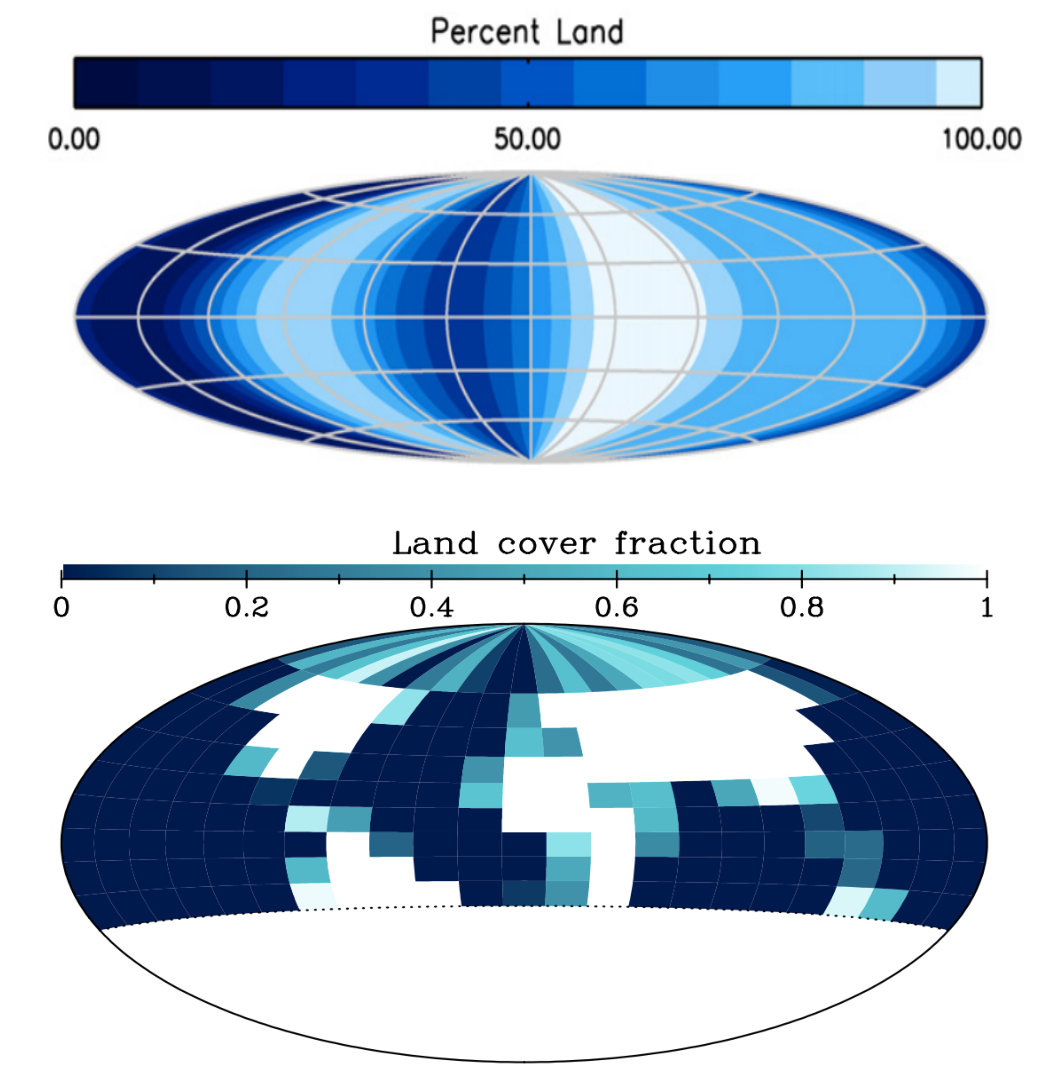 Figure 1
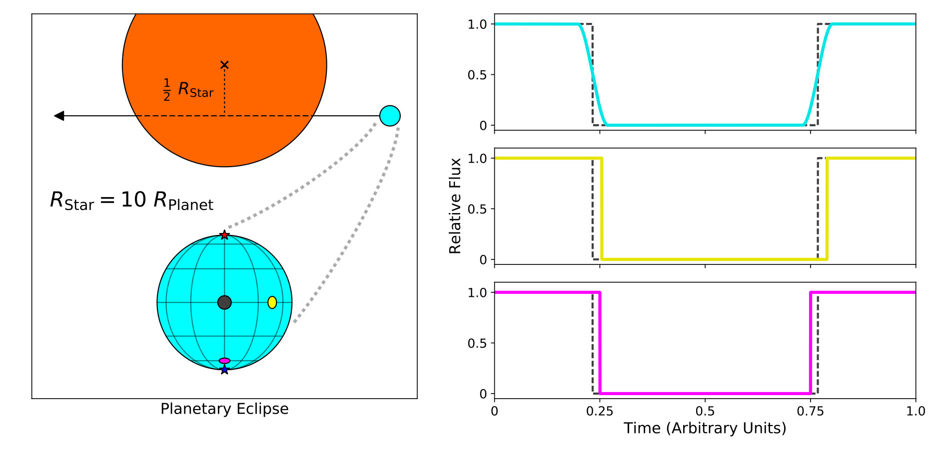 Figure 2
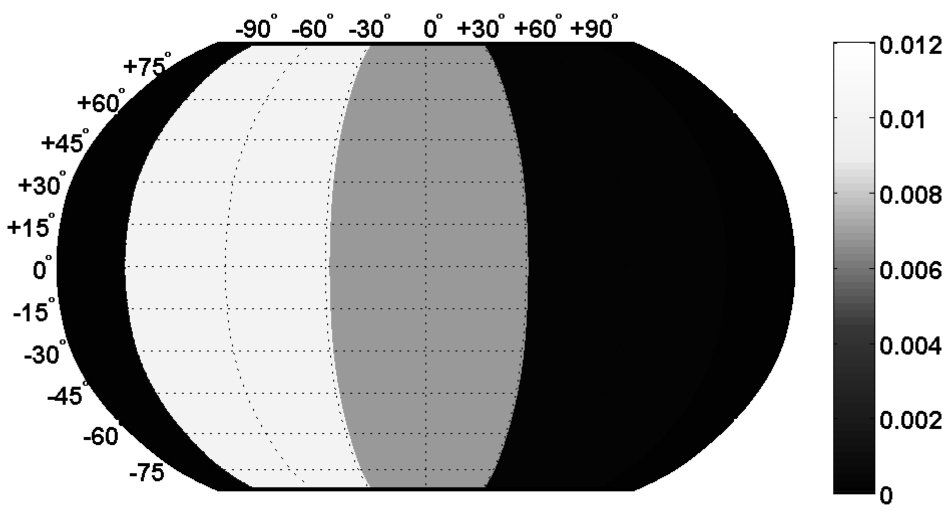 Figure 3
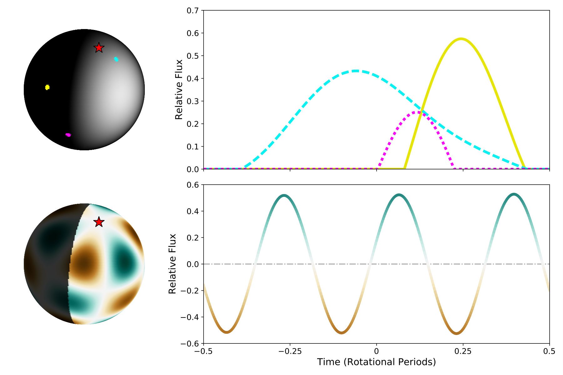 Figure 4
 Figure 4
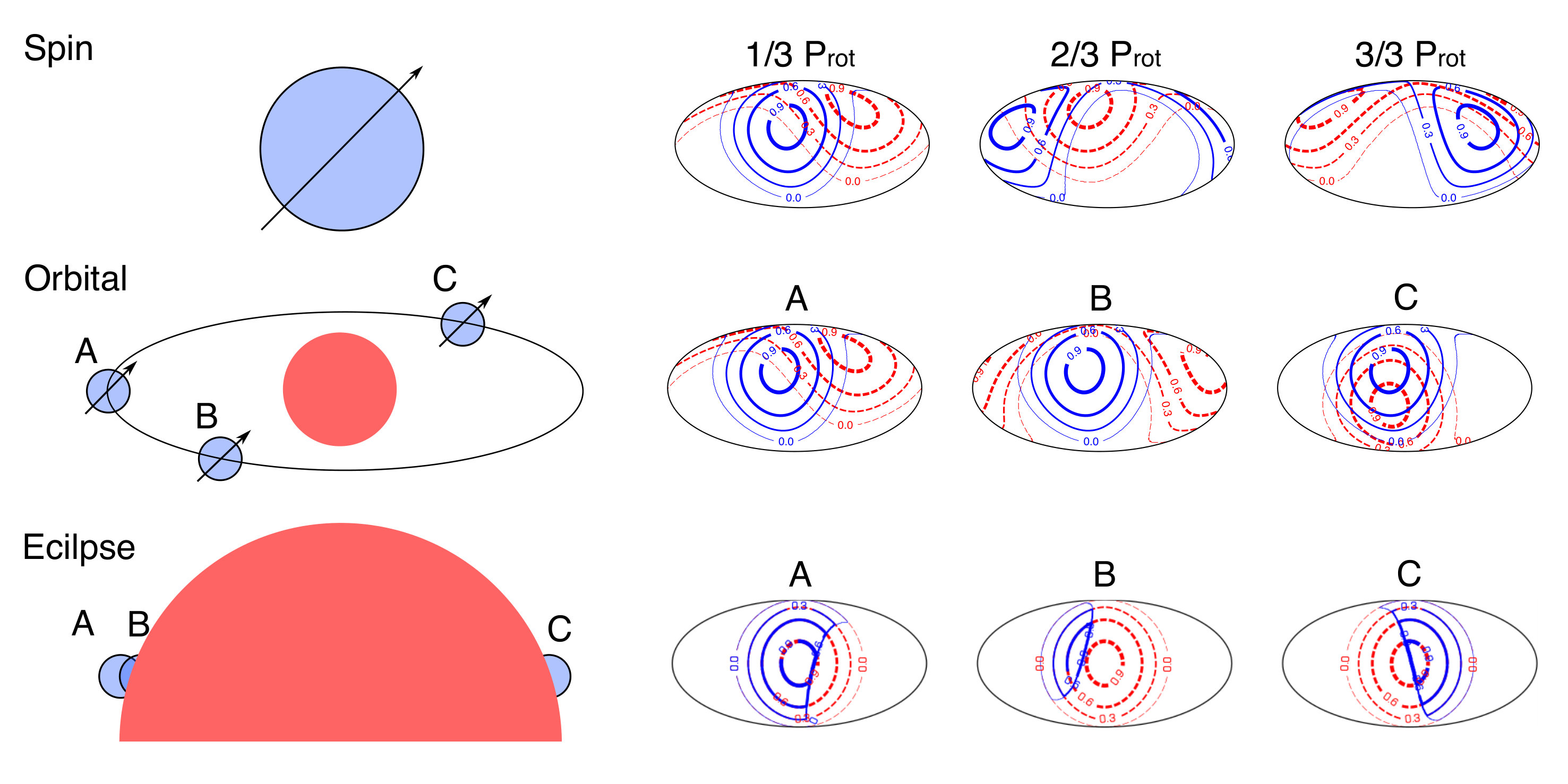 Figure 6
Peer Reviews
No public reviews on file for this paper yet. If you reviewed it on a platform where reviews are public (OpenReview, ICLR, NeurIPS, ICML), you can paste yours below so the community can read it here.
Videos
No videos yet. Explain this paper in a talk, walkthrough, or lecture? Add one.
11institutetext: Nicolas B. Cowan 22institutetext: McGill University, Montréal, Québec, Canada
22email: [email protected] 33institutetext: Yuka Fujii 44institutetext: National Astronomical Observatory of Japan, Mitaka, Tokyo, Japan
44email: [email protected]
Mapping Exoplanets
Nicolas B. Cowan and Yuka Fujii
Abstract
The varied surfaces and atmospheres of planets make them interesting places to live, explore, and study from afar. Unfortunately, the great distance to exoplanets makes it impossible to resolve their disk with current or near-term technology. It is still possible, however, to deduce spatial inhomogeneities in exoplanets provided that different regions are visible at different times—this can be due to rotation, orbital motion, and occultations by a star, planet, or moon. Astronomers have so far constructed maps of thermal emission and albedo for short period giant exoplanets. These maps constrain atmospheric dynamics and cloud patterns in exotic atmospheres. In the future, exo-cartography could yield surface maps of terrestrial planets, hinting at the geophysical and geochemical processes that shape them.
1 Introduction
Astronomy often involves studying objects so distant that they remain unresolved point sources with even the largest telescopes. Exoplanets are particularly difficult to study because they are small compared to other astronomical objects. The diffraction limit dictates that resolving the disk of an Earth-sized planet at 10 pc requires a telescope—or array of telescopes—at least 25 km across at optical wavelengths, or 500 km across in the thermal infrared. Short of building a large interferometer to spatially resolve the disks of exoplanets, we must rely on chance and astronomical trickery to map their atmospheres and surfaces.
We expect planets to have spatial inhomogeneities: left to their own devices, atmospheres are subject to instabilities that produce spatially and temporally varying temperature, composition, and aerosols. Moreover, planets orbiting a star are further subject to asymmetric radiative forcing from their star, leading to diurnal (day–night) and seasonal (summer–winter) variations. Lastly, the surface of a planet may have a heterogeneous character due to, e.g., plate tectonics or volcanism.
Although part of the motivation to map exoplanets is simply to know what they look like, there are undoubtedly cases where understanding a planet requires understanding the diversity of its different regions. On a short-period planet, for instance, the hot dayside atmospheres may have atomic and partially ionized gas, while the nightside may be hundreds to thousands of degrees cooler, often shrouded in clouds and sometimes entirely airless. Interpreting the disk-integrated light of a heterogeneous planet with a one-dimensional model is misleading (e.g., Feng et al. 2016). More importantly, the intrinsic climate of a planet is affected by its spatial inhomogeneities (Zhang 2023a, b; Zhang et al. 2023). We would therefore like to map the atmospheres and surfaces of exoplanets.
2 Mapping Basics
This chapter covers the analysis of planetary light, be it thermal radiation or reflected starlight. Planetary light can be separated from starlight temporally (Charbonneau et al. 2005; Deming et al. 2005), spatially (Marois et al. 2008), or spectrally (Brogi et al. 2012). Transmission mapping is also briefly described below.
It is possible to map the surface of an unresolved object as long as we don’t always see the same parts of it—the resulting changes in brightness can be detected across astronomical distances. We are therefore able to tease out spatial information about a planet based on its time-variable brightness, provided we know something about the viewing geometry. There are three ways in which our view of an exoplanet can change: rotation of the planet, changes in its position with respect to its star, and occultations by another object (Figure 1).
Rotational mapping is possible because at any given time, we only see light from at most a hemisphere and as the planet spins on its own axis, different atmospheric and surface features rotate in and out of view. Orbital mapping with reflected light is possible due to the changing illumination pattern as the planet orbits its star. Occultation mapping, on the other hand, requires a second object to obscure part of the planet—the host star is the most likely culprit—hence changing our view and the system’s overall flux. In practice, multiple sources of variability can be present in a single data set: phase variations are generally accompanied by rotation of the planet, and occultations are necessarily accompanied by orbital motion.
2.1 Transmission Mapping
It is also possible to glean spatial information about an exoplanet’s atmosphere when it transits in front of its host star: transmission mapping, or transit mapping. Transmission mapping shares some concepts with emission and reflection mapping, so is briefly described here. Transmission mapping relies on two geometrical facts: 1) only part of the planetary limb is backlit during transit ingress and egress, and 2) the planetary limb probed in transmission moves on the planet during a transit.
At the start of transit ingress, only the western (leading) limb of the planet is in front of the star and contributes to the transmission spectrum; likewise, the end of egress is only sensitive to the eastern (trailing) limb of the planet. Such transmission mapping has been proposed for detecting the difference in atmospheric scale height (Dobbs-Dixon et al. 2012), winds (Louden and Wheatley 2015), and aerosols (Kempton et al. 2017; Powell et al. 2019) near the eastern and western terminators. Many codes have been developed to perform such transmission mapping (Espinoza and Jones 2021; MacDonald and Lewis 2022; Grant and Wakeford 2023). The ingress-egress asymmetry is most marked for planets that are large compared to their star; the best spatial resolution could be obtained for a giant planet orbiting a white dwarf (e.g., Vanderburg et al. 2020). This phenomenon is conceptually similar to eclipse mapping, but is very sensitive to the limb-darkening of the star. Transmission mapping has already been performed with ground-based high resolution spectroscopy (Ehrenreich et al. 2020). Even in the middle of transit, high resolution data can differentiate between the blue-shifted eastern limb and and the red-shifted western limb (Boucher et al. 2023), analogous to Doppler imaging.
Moreover, the planet will rotate during the transit, i.e., the planetary limb does not exactly coincide with the day–night terminator. In fact, the limb only corresponds to the day–night terminator when the planet is in the center of the stellar disk, which never occurs for a non-zero impact parameter. At the start of transit the limb runs on the dayside of the eastern terminator and on the nightside of the western terminator, and vice versa at the end of transit. The angle between the limb and terminator is proportional to the angular size of the star as seen from the planet, and is therefore most important for ultra short period planets (Nguyen et al. 2020). If a rocky planet has a negligible atmosphere, then topographical features may rotate in and out of view during the transit (McTier and Kipping 2018). Transmission mapping of exoplanets is an exciting growth area, but the remainder of this review focuses on mapping exoplanets using light emitted or reflected by the planets themselves.
3 Mapping Formalism
Exo-cartography is an inverse problem, as opposed to the forward problem of predicting the spectrum of a planet based on its surface and atmospheric properties. The usual approach to an inverse problem is to solve the forward problem many times with varying parameters to see which ones best match the observations.
State-of-the-art forward modeling involves, at the very least, detailed radiative transfer calculations and hence is not useful for solving the inverse problem (Robinson et al. 2011). One of the necessities of tackling the inverse problem is therefore making judicious simplifications. Adopting the notation of Cowan et al. (2013), the exo-cartography forward problem is approximated as
[TABLE]
where is the observed flux, or lightcurve, is the convolution kernel, is the top-of-atmosphere planet map, and are planetary co-latitude and longitude, respectively, the differential solid angle is for a spherical planet, and is the integral over the entire planet. Although stands for “flux”, the units of depend on the situation and chosen normalization: planetary flux, planet/star flux ratio, reflectance, apparent albedo, etc.
Arguably the most important simplification is assuming a static map, , as it is generally intractable to map the surface of an unresolved planet when that map is changing. One can map a slowly varying planet, e.g., large-scale cloud patterns on Earth evolve slowly compared to the planet’s rotation (Kawahara and Masuda 2020; Teinturier et al. 2022) and some eccentric planets may still be amenable to eclipse mapping, despite seasonal variations. Beyond these exceptions, one must adopt a parameterized time-variable map, . For example, phase curves of eccentric hot Jupiters have been fitted with energy balance models (Lewis et al. 2013; de Wit et al. 2016; Dang et al. 2022). Finally, Cowan et al. (2017) showed that for planets on circular, edge-on orbits one can infer a time-variable map based on the presence of odd harmonics; nonetheless, this is a far cry from mapping the changing surface of a planet.
Barring a changing map, time-variations in flux come in through the kernel. If there are no occultations, then the changing sub-observer and sub-stellar locations dictate the time-variability of the kernel and hence the time-variations in observed flux.
3.1 The Inverse Problem
Inverse problems are often under-constrained, and exo-cartography is no exception: non-zero maps can produce flat lightcurves, a so-called nullspace, and different maps sometimes produce identical non-trivial lightcurves. These pitfalls represent the loss of information: attempts to map distant objects suffer from formal degeneracies, even in the limit of noiseless observations.
If the orientation of a planet is not known a priori, then the problem is even more challenging because the kernel is a function of one or more unknown parameters: spin frequency, spin orientation, etc. Nonetheless, it has been demonstrated in numerical experiments that one can extract a planet’s spin (rotation rate, obliquity and its direction) from reflected lightcurves (Pallé et al. 2008; Oakley and Cash 2009; Kawahara and Fujii 2010, 2011; Fujii and Kawahara 2012; Schwartz et al. 2016; Kawahara 2016; Farr et al. 2018; Nakagawa et al. 2020) or from thermal lightcurves (Gaidos and Williams 2004; Gómez-Leal et al. 2012; Cowan et al. 2012b, 2013). A similar formalism has been developed for imaging exoplanets with a solar gravitational lens (Toth and Turyshev 2023).
Exoplanets can be mapped in monochrome using single-band photometry, or using spectrally-resolved data to produce maps at each wavelength. It is often more insightful, however, to assume that the lightcurves are correlated due to viewing geometry, molecular absorption, or surface spectra. With high spectral resolution, for example, the signal is in the time-variable mean molecular line shape. We point the interested reader to the excellent review of high resolution atmospheric characterization (Birkby 2018) and note that much work remains to be done in extracting spatial information from high resolution data. The inverse problem of mapping a planet using template spectra—let alone retrieving intrinsic surface colors and spectra—based on multi-band photometry or time-resolved spectroscopy is beyond the scope of this review, but has been considered in the literature both in the context of reflected light (Cowan et al. 2009, 2011; Fujii et al. 2010, 2011; Cowan and Strait 2013; Fujii et al. 2017; Kawahara 2020) and thermal emission (Kostov and Apai 2013; Buenzli et al. 2014; Stevenson et al. 2014; Feng et al. 2016; Irwin et al. 2020; Changeat and Al-Refaie 2020; Cubillos et al. 2021).
4 Basis Maps and Basis Lightcurves
The exo-cartography inverse problem boils down to fitting observed lightcurves. One can use orthonormal basis maps, e.g., spherical harmonics,
[TABLE]
and repeatedly solve the forward problem in order to fit an observed lightcurve, or one can use orthonormal basis lightcurves, e.g., a Fourier series or eigencurves (Rauscher et al. 2018),
[TABLE]
to directly fit the observed lightcurve, then reconstruct the associated map and its uncertainties in post-processing. Sometimes, orthonormal basis maps produce orthonormal basis lightcurves and the problem is particularly tidy, as for rotational thermal mapping (Cowan and Agol 2008; Cowan et al. 2013). Usually, however, the adopted basis maps do not produce orthogonal lightcurves, and vice versa.
There are two broad classes of map parameterizations: global (e.g., spherical harmonics) and local (e.g., pixels). The optimal basis maps will depend on viewing geometry, expected map geometry, and the nature of the data (cf. Keating et al. 2019; Beatty et al. 2019). In general, spherical harmonics are better for rotational mapping, smoothly varying maps, and full phase coverage. Pixels are preferable for eclipse mapping, sharp features, or partial phase coverage. Apai et al. (2017) introduced hybrid basis maps to fit rotational lightcurves of brown dwarfs: zonal bands harboring sinusoidal waves.
It is advisable to adopt a basis for which some maps are constrained and others are unambiguously in the nullspace, as it makes degeneracies easier to track down. As with many inverse problems, priors on the model parameters can help stabilize fits, especially when the data are noisy. For exo-cartography, this takes the form of enforcing map positivity (Keating and Cowan 2017; Farr et al. 2018), regularization to favour smoothness between pixels (e.g., Knutson et al. 2007; Kawahara and Fujii 2010, 2011; Fujii and Kawahara 2012), suppressing power in high-order modes with a sharp cutoff (e.g., Cowan and Agol 2008; Majeau et al. 2012) or a Gaussian process (Farr et al. 2018; Kawahara and Masuda 2020; Luger et al. 2021).
4.1 Pixels and Slices
An intuitive approach is to pixelize the planetary surface. The most general pixelization scheme is 2-dimensional, for example, a latitude–longitude grid or Hierarchical Equal Area isoLatitude Pixelization (HEALPix), but more exotic schemes have been developed for occultation mapping (Louden and Kreidberg 2018). Pixels are useful if the kernel moves or changes its shape in more than one direction, e.g., eclipse mapping or rotational reflected light curves at multiple orbital phases.
Denoting the intensity of the pixel by , we may express an arbitrary map as
[TABLE]
where the basis maps are
[TABLE]
As small pixel is well approximated by a -function at its center. Although -functions are terrible for decomposing continuous maps, they have the advantage of being trivial to integrate (Haggard and Cowan 2018):
[TABLE]
For rotational mapping, latitudinal information is difficult to extract, so it is often reasonable to consider a map consisting of uniform slices, like a beach ball. This situation includes rotational mapping in the thermal infrared (Knutson et al. 2007) and rotational mapping of reflected light at a fixed orbital phase (Cowan et al. 2009).
4.2 Spherical Harmonics
A continuous albedo map, , may be decomposed into spherical harmonics:
[TABLE]
where the coefficients are
[TABLE]
It is difficult to extract latitudinal information from purely rotational variations (the little that can be squeezed out is described by Cowan et al. 2013, 2017). It is expedient in such cases to adopt sinusoidal basis maps (Cowan and Agol 2008), essentially spherical harmonics with .
4.3 The Kernel
The kernel is the equivalent to the vertical contribution function in 1D atmospheric radiative transfer (Kawahara and Fujii have used “weight” instead of “kernel”). By definition, the kernel must move over the planet in order for exo-cartography to be possible. The shape of the kernel, however, is constant for rotational mapping and thermal phase mapping. For such a static kernel, some maps are always in the nullspace, leading to severe degeneracy in the inverse problem (Cowan et al. 2013). If the shape of the kernel changes with time, then maps need not remain in the nullspace, e.g., eclipse mapping (Challener and Rauscher 2023), or reflected-light mapping involving both rotation and orbital motion (Haggard and Cowan 2018). The degeneracy-busting power of a changing kernel is analogous to how a changing antenna pattern reduces the degeneracy in the location of a radio source on the sky.
Thermal Emission
For diffuse thermal emission, the kernel is simply the normalized visibility:
[TABLE]
where the visibility, , is unity at the sub-observer location (the center of the planetary disk as seen by the observer), drops as the cosine of the angle from the sub-observer location if limb-darkening can be neglected, and is zero on the far side of the planet or any part of the planet hidden from view by an occulting object. Cowan et al. (2013) derived analytic orbital/rotational lightcurves for spherical harmonic basis maps and Luger et al. (2019a) did the same for occultations.
Due to the unchanging kernel shape for rotational or orbital thermal mapping, a large fraction of spherical harmonics are in the nullspace, limiting the fidelity of retrieved maps. A common strategy is to ignore basis maps in the nullspace, setting their amplitude to zero in fits (Cowan and Agol 2008). But this strategy can sometimes produce retrieved maps that appear to have regions of negative flux, an artifact of the band-limited deconvolution. The solution is to fit for more basis maps—including those in the nullspace: immeasurable fitted parameters may help the map remain everywhere positive (Keating et al. 2019). Such hidden variables can be further constrained by a regularization scheme or Gaussian process. Indeed, the most general and robust approach to mapping is likely a high-order orthogonal map expansion—many spherical harmonics or pixels—embedded in a hierarchical model (Farr et al. 2018; Luger et al. 2021). If the prospect of fitting unseen and unknowable parameters by relying on priors is daunting, rest assured that you can often obtain a good fit and reasonable map by adopting an altogether different parameterization, such as slices or pixels (Beatty et al. 2019).
Reflected Light
For diffuse reflected light (a.k.a. Lambertian reflection), the kernel is the product of visibility and illumination:
[TABLE]
where the visibility is defined as above, and the illumination is unity at the sub-stellar location (the center of the planetary disk as seen from the star), drops as the cosine of the angle from the sub-stellar location, and is zero on the night side of the planet or any part of the planet in the shadow of another object (e.g., an eclipsing planet or moon). Analytic reflected lightcurves have so far been derived for spherical harmonic maps at full phase (Russell 1906), for tidally-locked, edge-on geometry (Cowan et al. 2013), for the general case of an unocculted planet (Haggard and Cowan 2018), and finally including occultations (Luger et al. 2022). Extending this framework to polarized reflected light is beyond the scope of this review, but would undoubtedly yield useful constraints on cloud and surface properties (for a review of exoplanet polarimetry, see Wiktorowicz and Stam 2015).
The Lambertian scattering approximation is suitable for mapping gibbous planets (Fujii and Kawahara 2012), but preferential back-scattering can be important at full phase, while forward scattering and specular reflection are important at crescent phases (Robinson et al. 2010). If specular reflection is the dominant form of reflection, then the kernel is approximately a -function at the location of the glint spot, making the forward problem analytically tractable (Haggard and Cowan 2018). Specular reflection from surface liquid water is important as it is a direct indication of habitability (Robinson et al. 2014, and chapter by Tyler Robinson). Combining Lambertian mapping at gibbous phases with glint mapping at crescent phases would provide strong evidence for surface liquids (Lustig-Yaeger et al. 2018): oceans appear dark at most phases, but bright when specularly reflecting grazing sunlight (especially in polarized light; Groot et al. 2020).
Occultations
If a planet passes directly behind its star, then one may map its day side. Eclipse mapping can be applied to either planetary emission or reflected light, but the contrast ratio makes the latter daunting. While the eclipse depth is proportional to the integrated day side brightness of the planet, the detailed shape of ingress and egress is a function of the spatial distribution of flux on the planet’s day side (Figure 3). Although eclipses of planets by their host star have so far garnered the most attention, occultations by moons or other planets are also possible, especially in packed planetary systems like TRAPPIST-1 (Veras and Breedt 2017; Luger et al. 2017).
Fast codes are now available to produce occultation lightcurves numerically (SPIDERMAN; Louden and Kreidberg 2018) and analytically (starry; Luger et al. 2019a). The sharp kernel edge during an occultation—the stellar limb—increases the spatial resolution achievable in eclipse maps, and a larger impact parameter provides better latitudinal resolution (Boone et al. 2023).
5 Current Results & Future Prospects
The atmospheres of a few dozen exoplanets have been mapped via their thermal phase curves, e.g., the ExoAtmospheres and exoplanet.edu databases. These phase measurements has so far been mostly IRAC photometry from the Spitzer Space Telescope (e.g., Bell et al. 2021; May et al. 2022), or spectroscopy with the Hubble Space Telescope’s WFC3 (e.g., Stevenson et al. 2014; Kreidberg et al. 2018). We send the interested reader to the brief history of thermal phase curves in Charnay et al. (2022). Phase measurements from the James Webb Space Telescope have started being published, but so far focusing primarily on photometry (Mikal-Evans et al. 2023; Bell et al. 2023; Kempton et al. 2023). Rotational phase variations of brown dwarfs have also been measured and converted into brightness maps (e.g., Apai et al. 2017, and chapter by Artigau).
The Ariel mission could measure spectroscopic phase curves for dozens—if not hundreds—of planets and brown dwarfs (Charnay et al. 2022). The wavelength coverage of Ariel and JWST should be able to discriminate between thermal emission and reflected light (Schwartz and Cowan 2015; Parmentier et al. 2016; Keating and Cowan 2017), as well as disentangling phase variations, star spots, Doppler beaming, ellipsoidal variations, and gas accretion (Cowan et al. 2012a; Knutson et al. 2012; Esteves et al. 2015; Dang et al. 2018; Bell et al. 2019).
Eclipse mapping of hot Jupiters has so far been performed with Spitzer/IRAC photometry (Majeau et al. 2012; de Wit et al. 2012) and JWST/NIRISS spectroscopy (Coulombe et al. 2023). Figure 4 shows the combined phase+eclipse map of HD 189733b from Majeau et al. (2012) showing both longitudinal and latitudinal information, making this a coarse 2D map. The high signal-to-noise and spectral resolution of JWST should enable 3D temperature maps of the daysides of hot Jupiters, and 2D (longitude and altitude) temperature maps of their nightsides. Eclipse mapping of longer-period planets, which may not be tidally locked, could reveal their spin axis (Rauscher 2017; Adams and Rauscher 2023; Rauscher et al. 2023).
Ground-based direct imaging could detect variations in thermal emission from directly-imaged planets due to rotation of patchy clouds in and out of view (Biller et al. 2021), as is currently performed for brown dwarfs. The next generation of ground based telescopes should enable both photometric mapping and Doppler tomography of giant planets (Crossfield et al. 2014), while the Large Interferometer for Exoplanets (Quanz et al. 2022) could map the climates of temperate terrestrial planets (e.g., Gaidos and Williams 2004; Cowan et al. 2012c; Mettler et al. 2023).
Demory et al. (2013) constructed an albedo map of the hot Jupiter Kepler-7b based on phase curves from the Kepler mission (Fig. 5). NASA’s Grace Roman Space Telescope will directly image Jupiter analogs in reflected light, hence enabling rotational mapping of their clouds. The Habitable Worlds Observatory will enable reflected light surface mapping and spin determination for terrestrial planets (Figure 6; Ford et al. 2001; Pallé et al. 2008; Oakley and Cash 2009; Cowan et al. 2009, 2011; Kawahara and Fujii 2010, 2011; Fujii and Kawahara 2012; Cowan and Strait 2013; Schwartz et al. 2016; Kawahara 2016; Fujii et al. 2017; Jiang et al. 2018; Farr et al. 2018; Luger et al. 2019b; Fan et al. 2019; Kawahara 2020; Aizawa et al. 2020; Nakagawa et al. 2020).
Surface water is the definition of planetary habitability (Kasting et al. 1993), while the bimodal surface character of Earth—large oceans and exposed continents—may be crucial to its long-term habitability (Walker et al. 1981; Abbot et al. 2012; Foley 2015, 2019; Dorn et al. 2018; Foley and Smye 2018; Höning et al. 2019). Constructing surface maps of terrestrial exoplanets will therefore be a step towards understanding habitable environments outside of the Solar System and indeed to finding inhabited worlds (for a review see Suto 2019).
Clouds are a blessing and a curse to exo-cartography. From Earth to brown dwarfs, clouds contribute to the spatial inhomogeneity that make exo-cartography interesting and feasible. But clouds also mask underlying features and often vary in time. Ongoing efforts are demonstrating how to map clouds and devising schemes to minimize their effects (Cowan et al. 2009; Cowan and Strait 2013; Fujii et al. 2017; Jiang et al. 2018) in order to catch glimpses of the planetary surface below (Kawahara and Masuda 2020; Teinturier et al. 2022).
Acknowledgements.
The authors are grateful to International Space Science Institute for hosting the Exo-Cartography workshops (2016–2017) during which the first version of this review was drafted. N.B. Cowan acknowledges the financial support and stimulating environment of the Trottier Space Institute and l’Institut de recherche sur les exoplanètes. The authors thank J.C. Schwartz for creating many of the figures, as well as T. Bell, D. Keating, E. Rauscher, and T. Robinson for providing useful feedback on an earlier draft of this review.
Cross-References
- •
“Detecting Habitability”
- •
“Characterization of Exoplanets: Secondary Eclipses”
- •
“Characterization of Exoplanets: Observations and Modeling of Orbital Phase Curves”
- •
“Variability of Brown Dwarfs”
- •
“Spectroscopic Direct Detection of Exoplanets”
The reference list from the paper itself. Each links out to its DOI / PubMed record.
- 1Abbot et al. (2012) Abbot DS, Cowan NB Ciesla FJ (2012) Indication of Insensitivity of Planetary Weathering Behavior and Habitable Zone to Surface Land Fraction. Ap J 756:178
- 2Adams and Rauscher (2023) Adams AD Rauscher E (2023) The Sensitivity of Eclipse Mapping to Planetary Rotation. AJ 165(1):24
- 3Agol et al. (2010) Agol E, Cowan NB, Knutson HA et al. (2010) The Climate of HD 189733 b from Fourteen Transits and Eclipses Measured by Spitzer. Ap J 721:1861–1877
- 4Aizawa et al. (2020) Aizawa M, Kawahara H Fan S (2020) Global Mapping of an Exo-Earth Using Sparse Modeling. Ap J 896(1):22
- 5Apai et al. (2017) Apai D, Karalidi T, Marley MS et al. (2017) Zones, spots, and planetary-scale waves beating in brown dwarf atmospheres. Science 357(6352):683–687
- 6Beatty et al. (2019) Beatty TG, Marley MS, Gaudi BS et al. (2019) Spitzer Phase Curves of KELT-1b and the Signatures of Nightside Clouds in Thermal Phase Observations. AJ 158(4):166
- 7Bell et al. (2019) Bell TJ, Zhang M, Cubillos PE et al. (2019) Mass loss from the exoplanet WASP-12b inferred from Spitzer phase curves. MNRAS 489(2):1995–2013
- 8Bell et al. (2021) Bell TJ, Dang L, Cowan NB et al. (2021) A comprehensive reanalysis of Spitzer’s 4.5 μ 𝜇 \mu m phase curves, and the phase variations of the ultra-hot Jupiters MASCARA-1b and KELT-16b. MNRAS 504(3):3316–3337