Measuring surface magnetic fields of red supergiant stars
Benjamin Tessore, Agn\`es L\`ebre, Julien Morin, Philippe Mathias,, Eric Josselin, and Michel Auri\`ere

TL;DR
This study investigates surface magnetic fields in a sample of red supergiant stars, finding weak magnetic signatures in several stars and suggesting magnetic fields are common in such stars but may diminish in later evolutionary stages.
Contribution
The paper extends the detection of surface magnetic fields to multiple M-type supergiants, demonstrating that weak magnetic fields are prevalent among these stars and analyzing their variability.
Findings
Weak Zeeman signatures detected in CE Tau, α¹ Her, and μ Cep.
Magnetic fields at the Gauss level in CE Tau and μ Cep.
Variability of magnetic fields correlates with atmospheric dynamics.
Abstract
RSG stars are very massive cool evolved stars. Recently, a weak magnetic field was measured at the surface of Ori and this is so far the only M-type supergiant for which a direct detection of a surface magnetic field has been reported. By extending the search for surface magnetic field in a sample of late-type supergiants, we want to determine whether the surface magnetic field detected on Ori is a common feature among the M-type supergiants. With the spectropolarimeter Narval at TBL we undertook a search for surface magnetic fields in a sample of cool supergiant stars, and we analysed circular polarisation spectra using the least-squares deconvolution technique. We detect weak Zeeman signatures of stellar origin in the targets CE Tau, Her and Cep. For the latter star, we also show that cross-talk from the strong linear polarisation signals detected on…
Click any figure to enlarge with its caption.
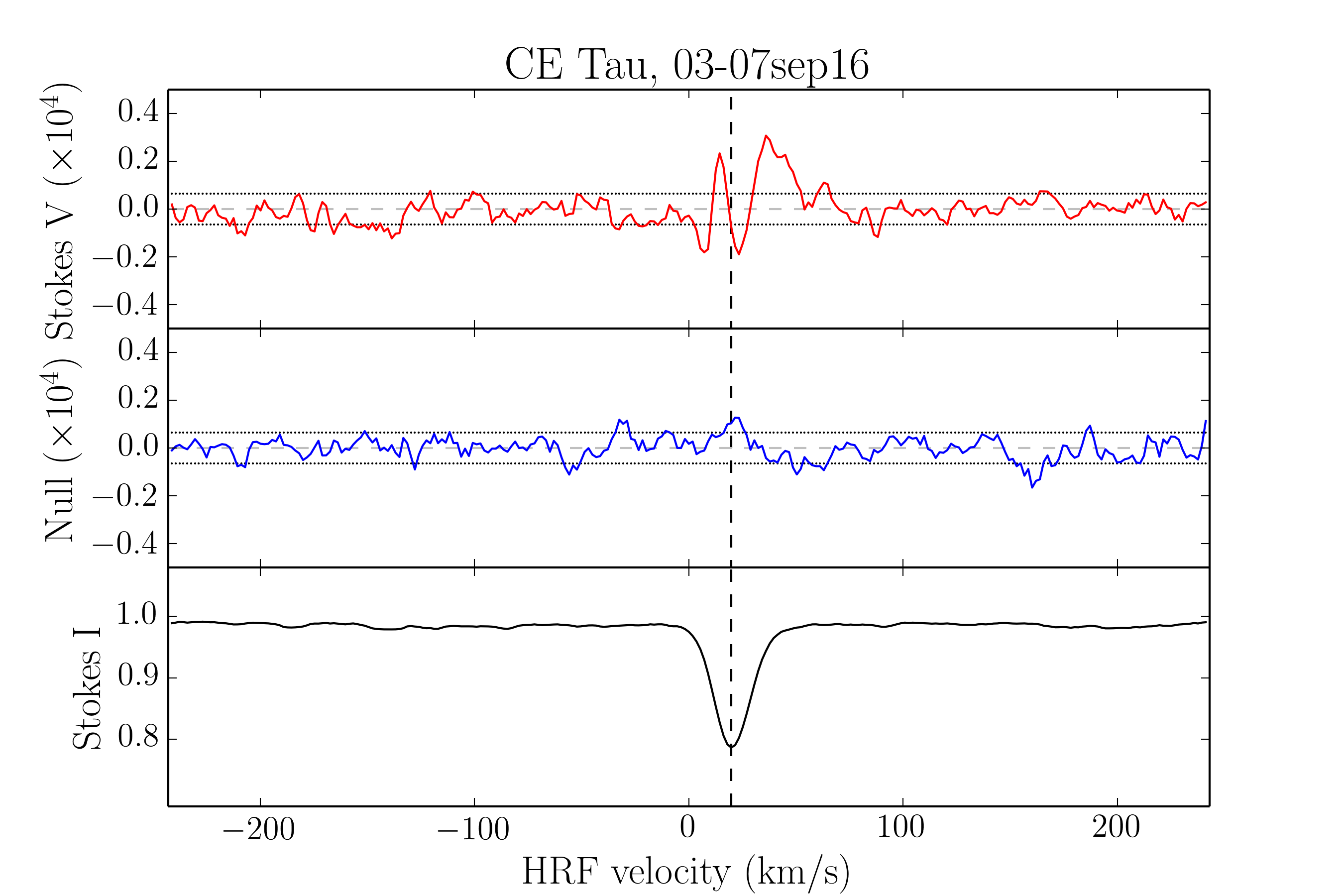 Figure 1
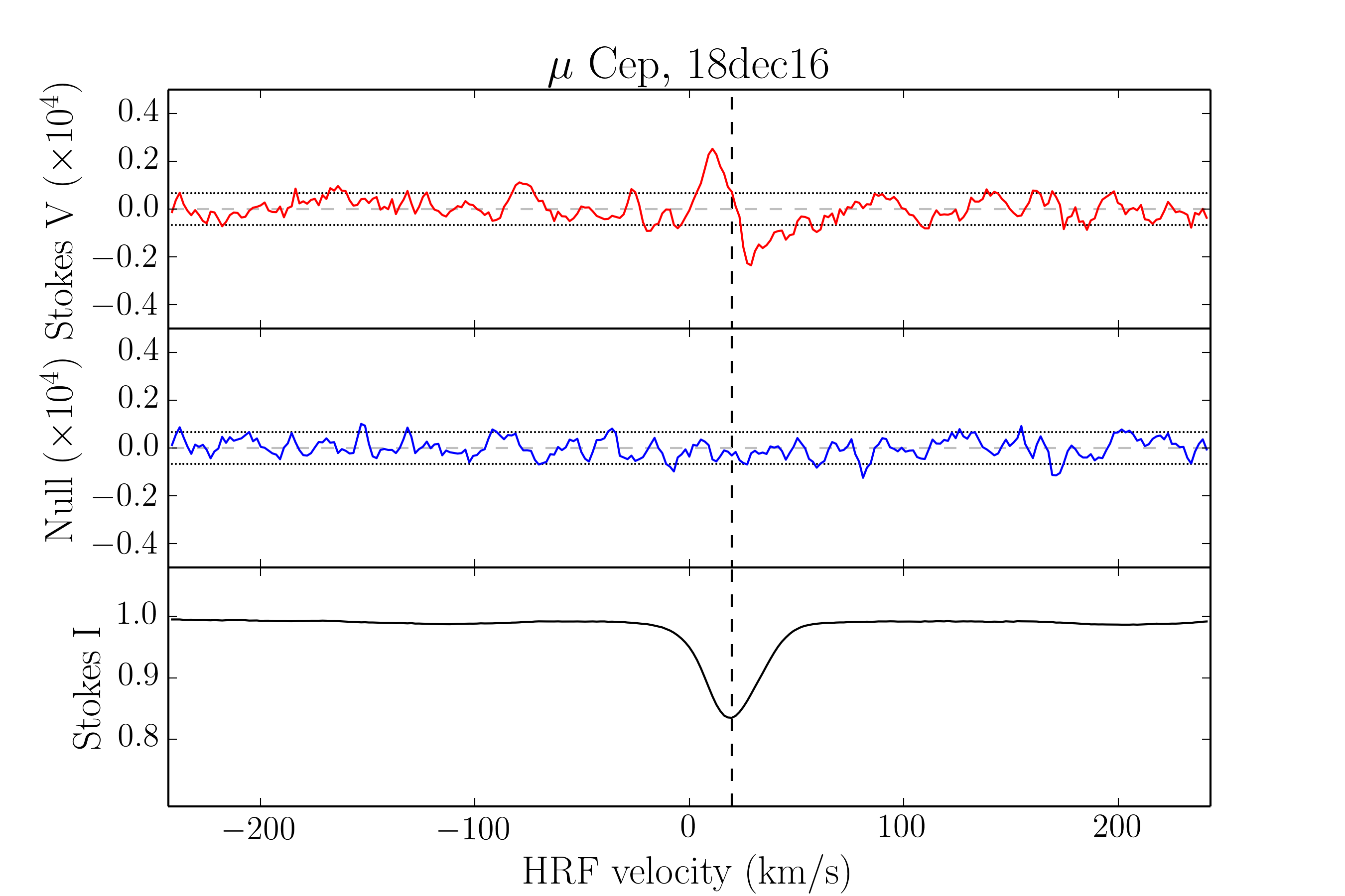 Figure 1
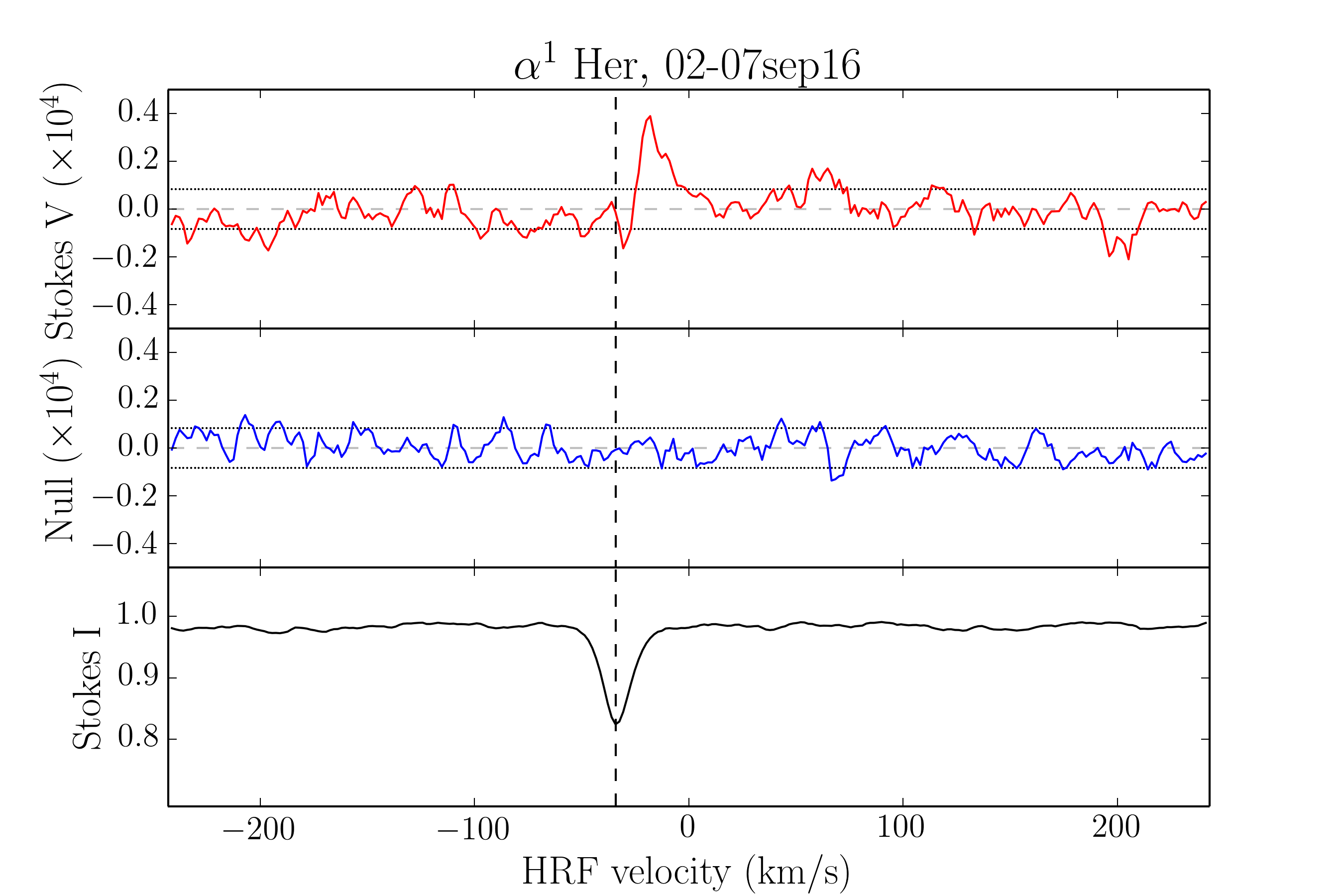 Figure 1
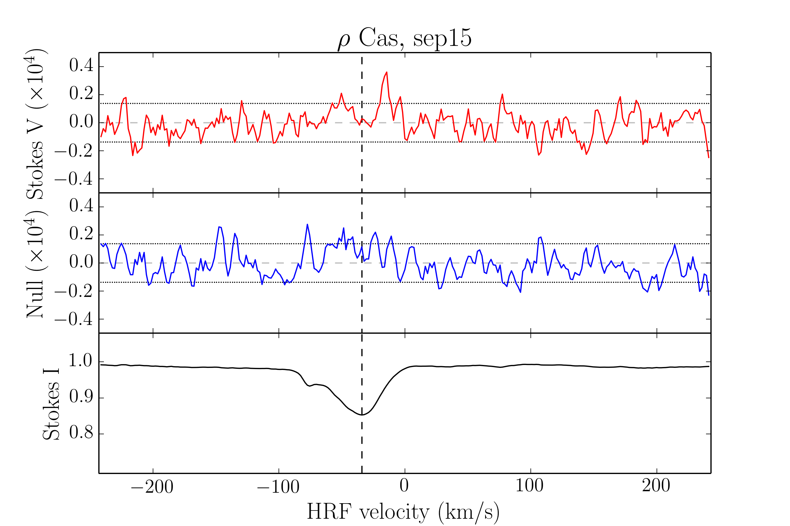 Figure 1
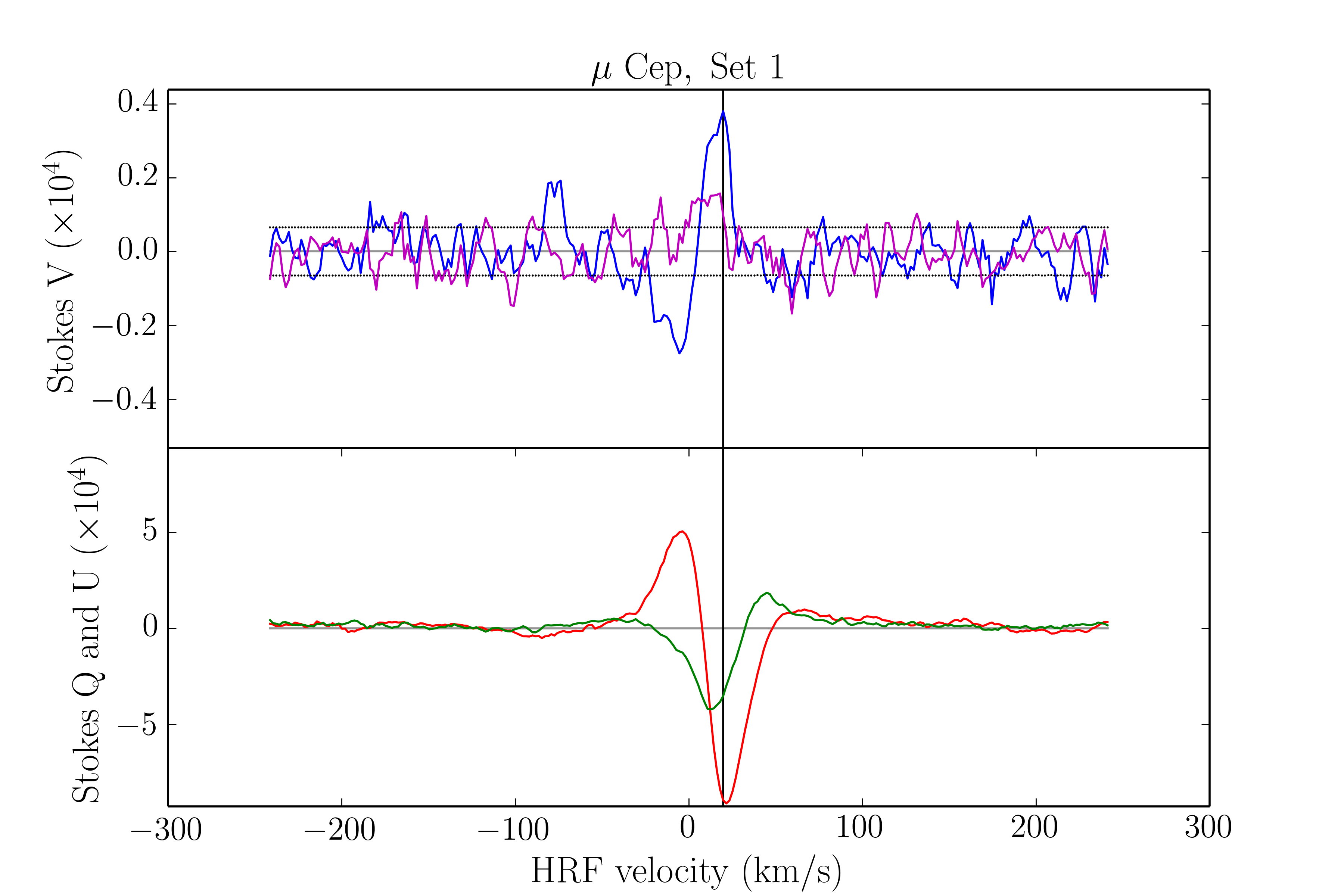 Figure 2
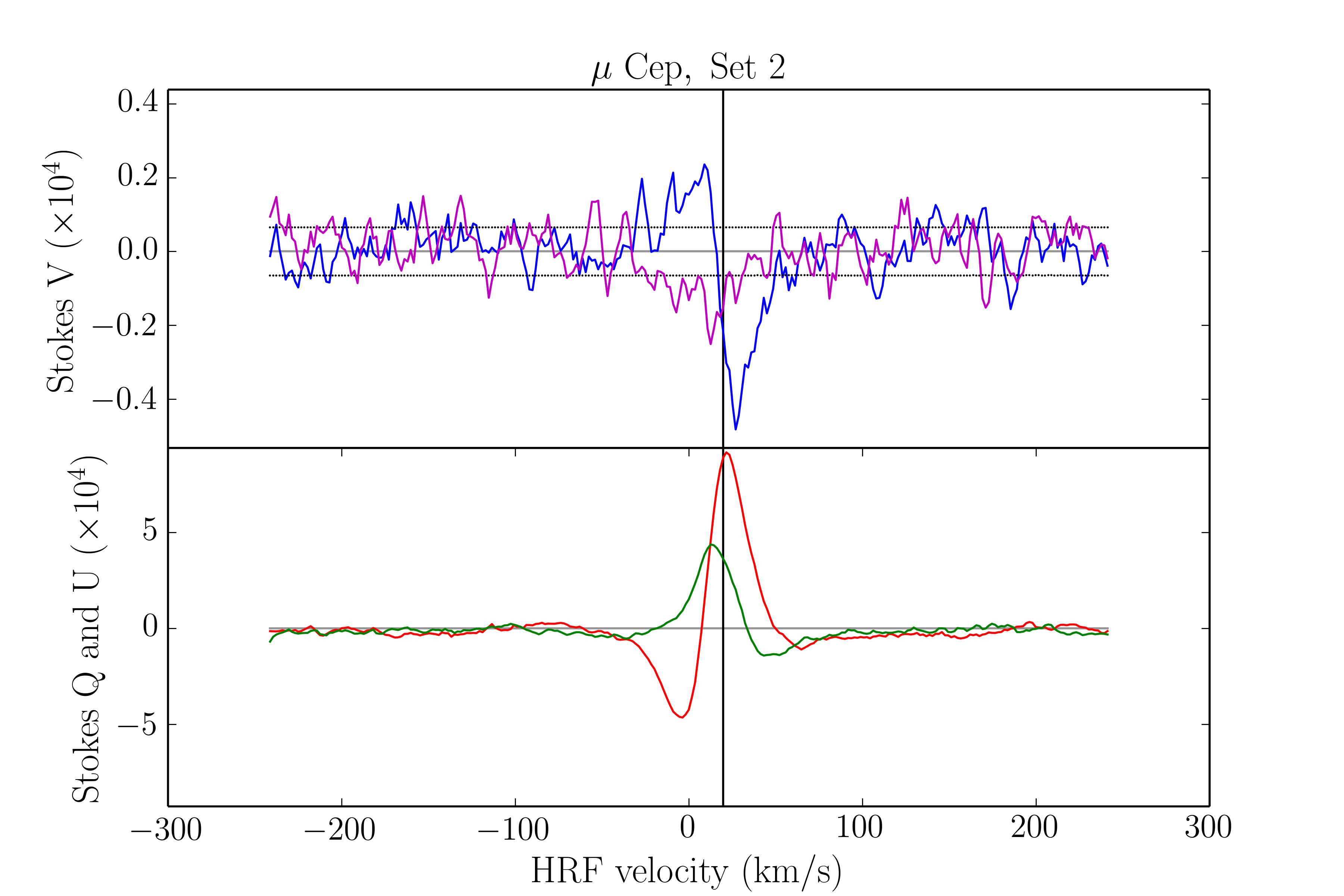 Figure 2
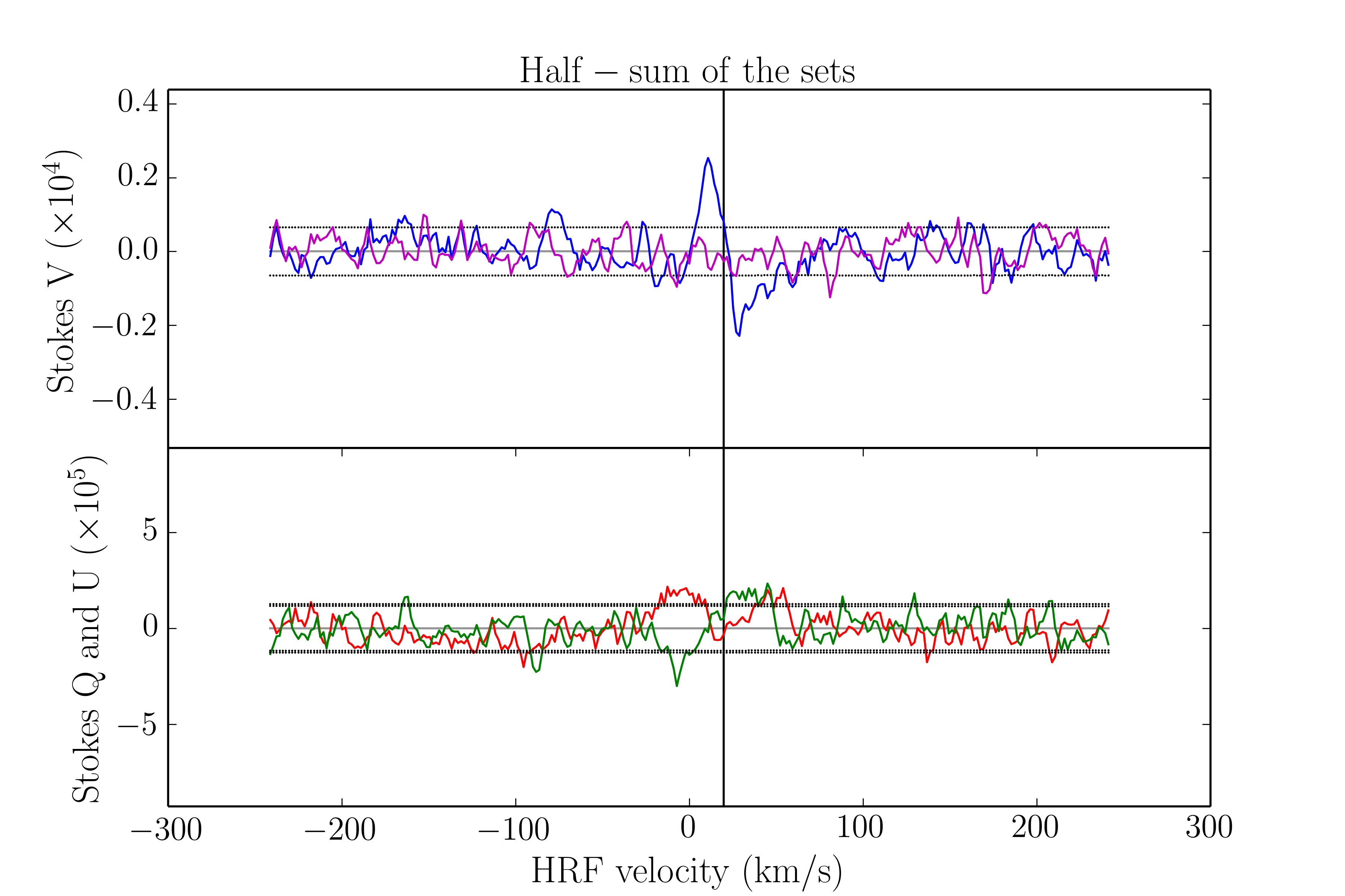 Figure 3
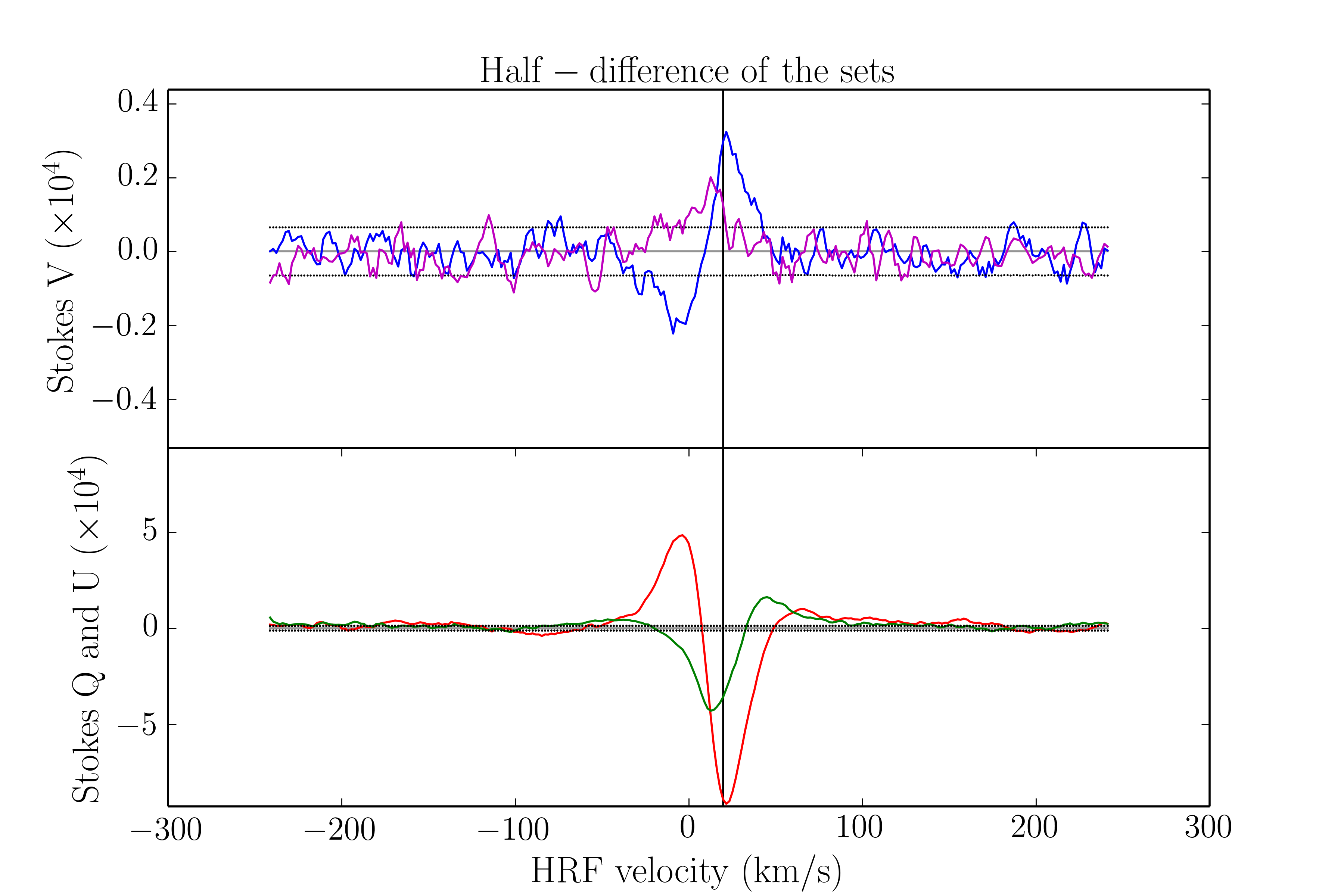 Figure 3
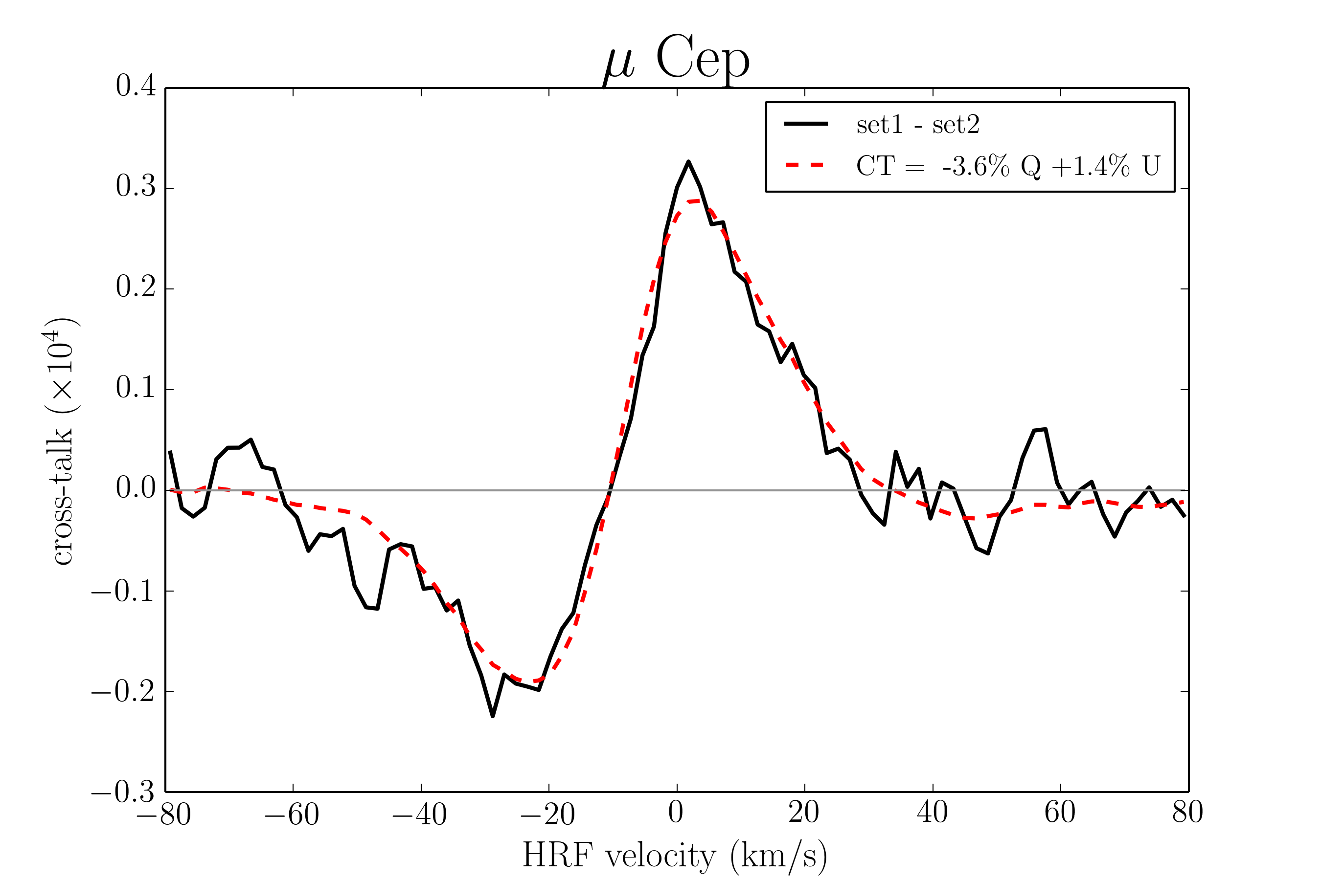 Figure 4
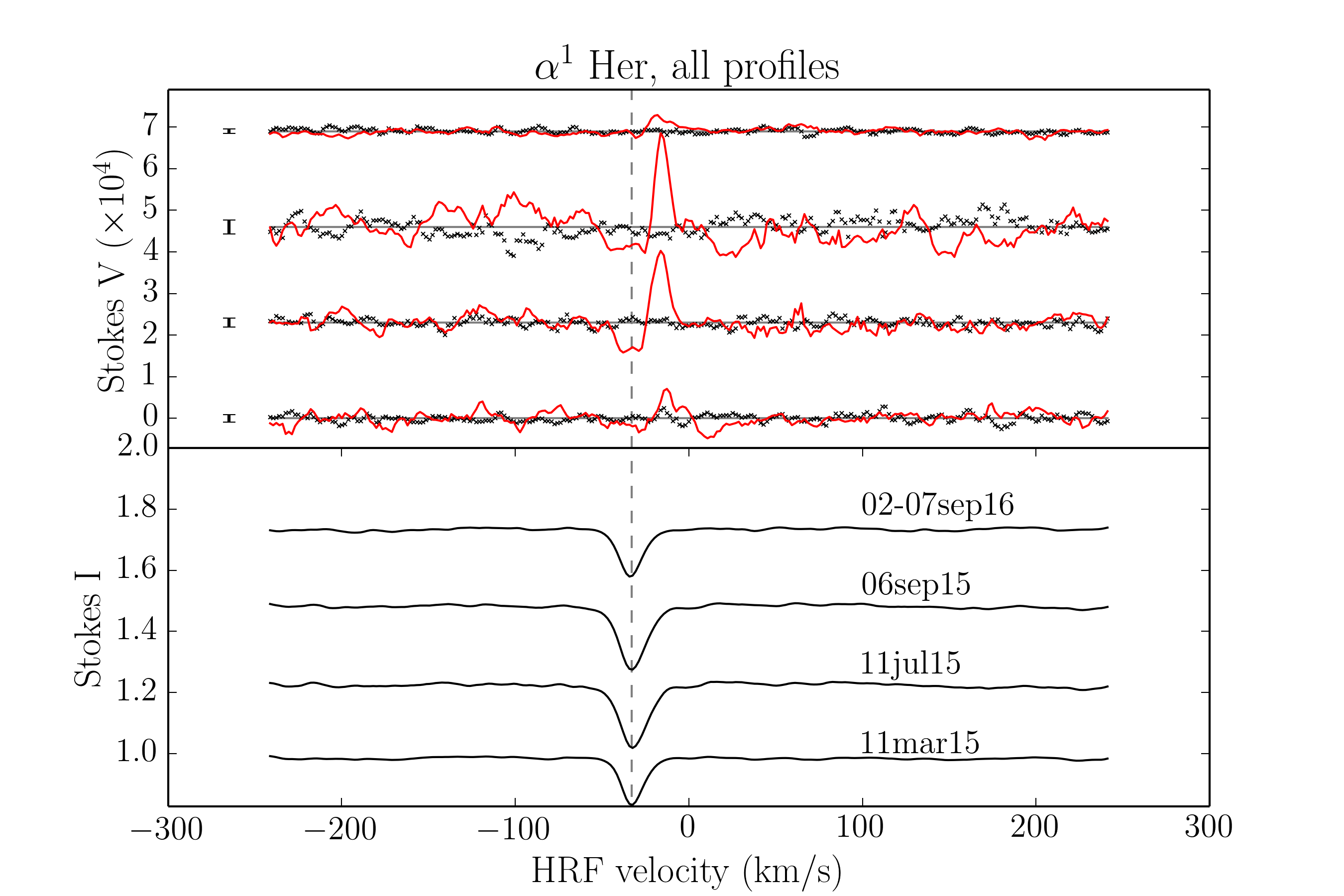 Figure 5
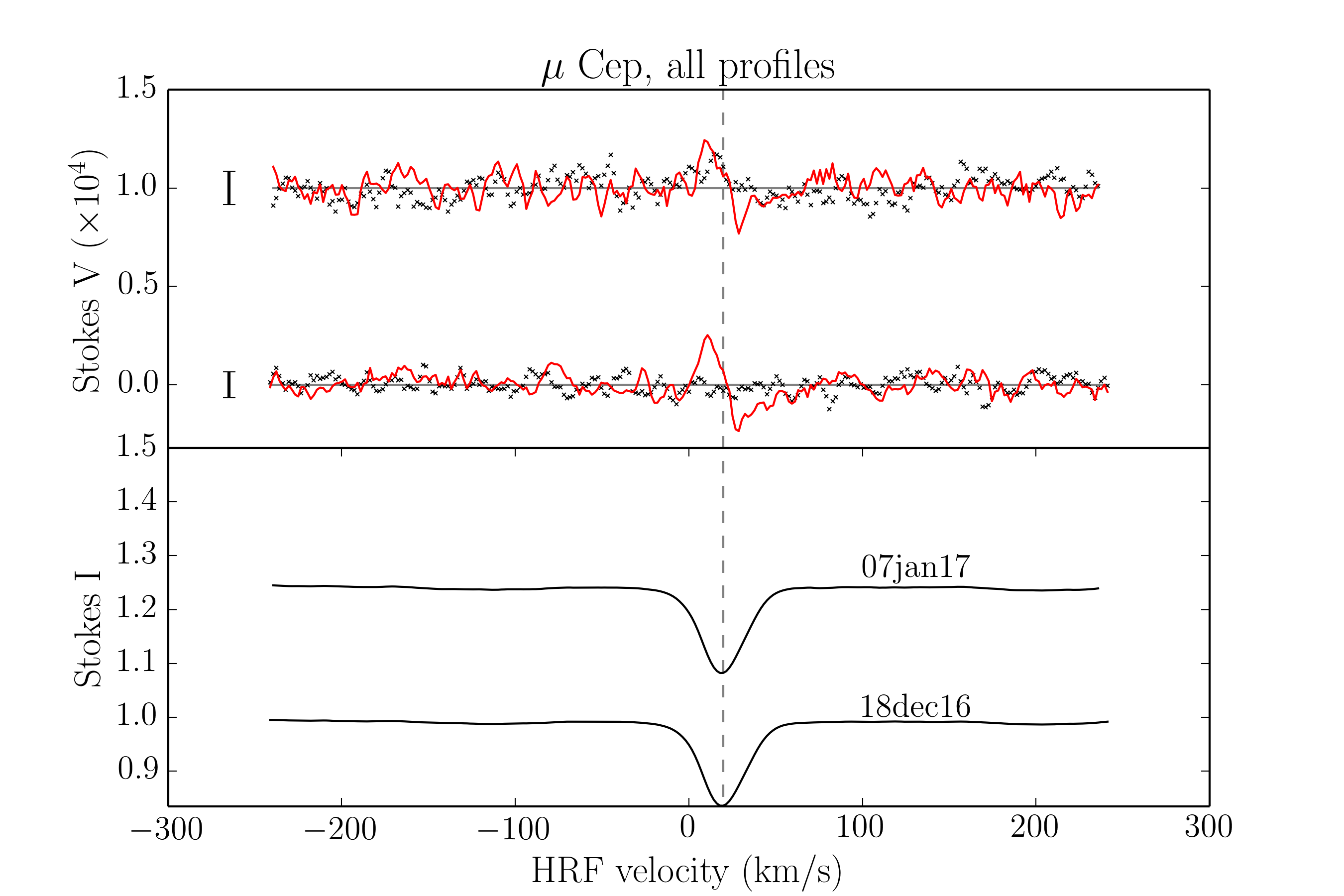 Figure 5
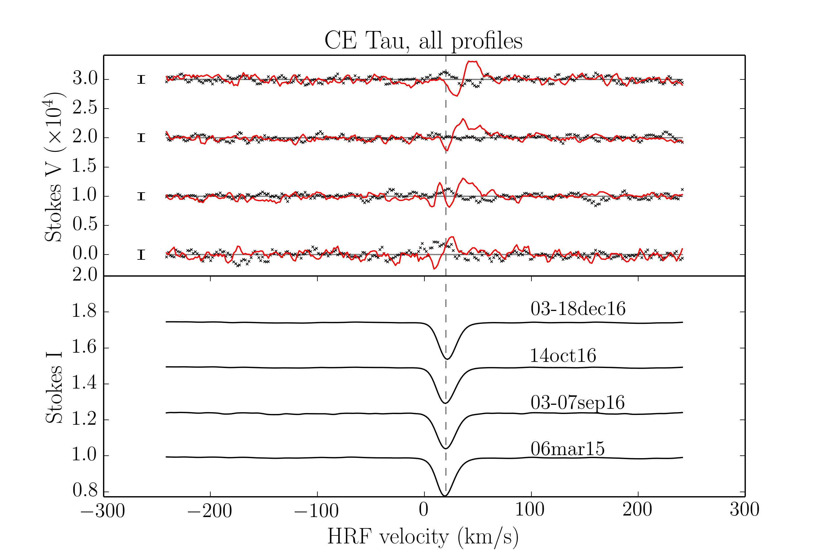 Figure 5
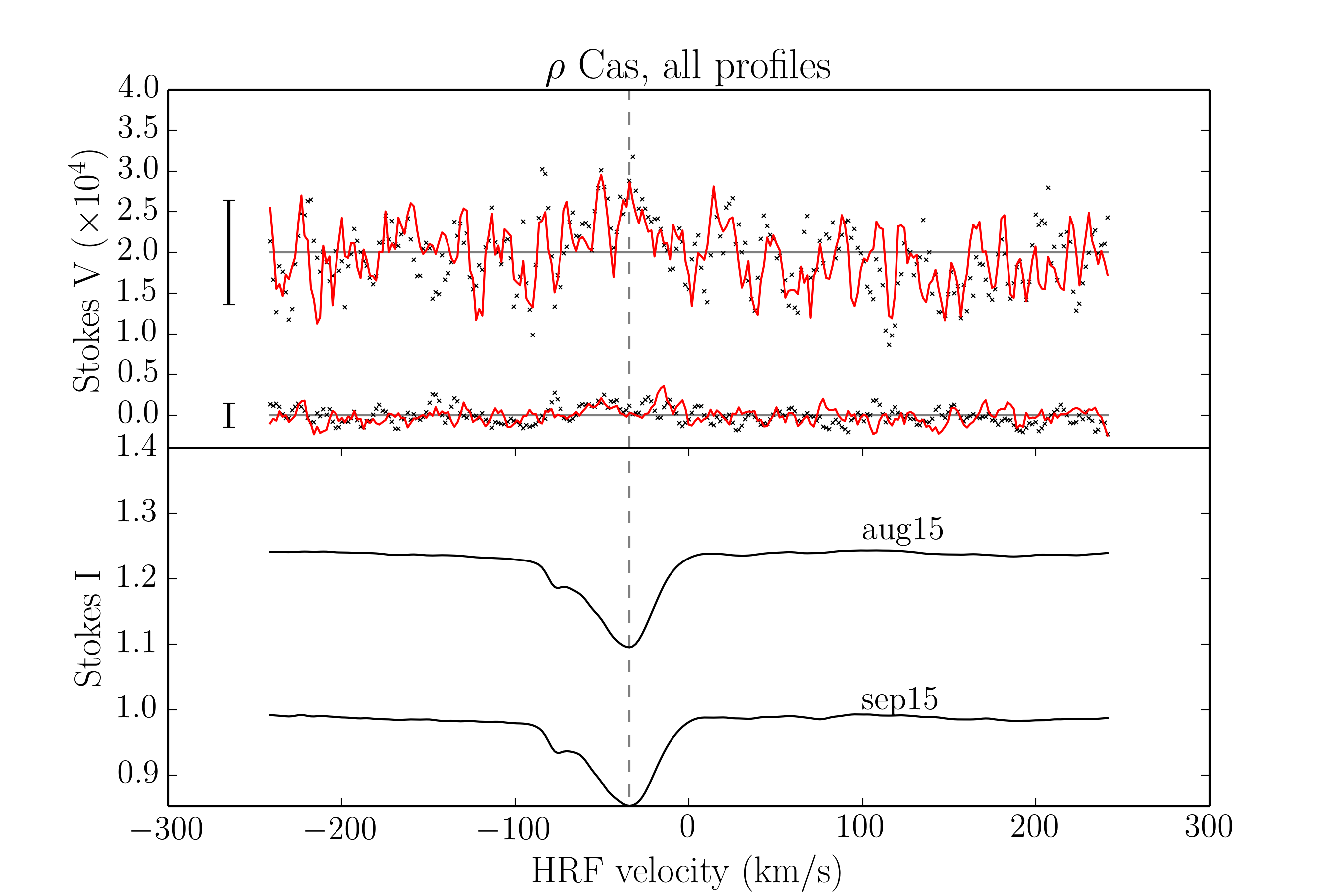 Figure 5
| Target | Spectral type | (K) | |||
|---|---|---|---|---|---|
| M2eIa | 3750 | -0.36 | 4.10 | 25 | |
| M5Ib-II(+G8III+A9IV-V) | 3280 | 0.0 | 3.35 | 2.5 | |
| M2Iab-Ib | 3510 | 0.0 | 4.30 | 15 | |
| G2Ia0e | 6000 | 0.25 | 4.59 | - | |
| M1-M2Ia-ab | 3780 | 0.08 | 0.42 | 15 |
| Target | Julian dates (HJD-2,400,000.5) | Dates (yyyy-mm-dd) | Exposure time (s) | Sequences | SNR peak (/2.6 bin) |
| 57 213.1 | 2015-07-09 | 200 | 16 | 1740 | |
| 57 266.9 | 2015-09-01 | 200 | 25 | 1550 | |
| 57 309.9 | 2015-10-14 | 200 | 25 | 1391 | |
| 57 337.9 | 2015-11-11 | 200 | 25 | 1542 | |
| 57 740.8 | 2016-12-18a | 200 | 8 | 1695 | |
| 57 760.8 | 2017-01-07 | 200 | 8 | 1749 | |
| 57 093.1 | 2015-03-11 | 120 | 16 | 2122 | |
| 57 214.9 | 2015-07-11 | 120 | 16 | 2069 | |
| 57 271.8 | 2015-09-06 | 120 | 9 | 1970 | |
| 57 633.9 | 2016-09-02 | 120 | 5 | 1842 | |
| 57 634.8 | 2016-09-03 | 120 | 11 | 1632 | |
| 57 636.9 | 2016-09-05 | 120 | 5 | 1177 | |
| 57 637.9 | 2016-09-06 | 120 | 7 | 1537 | |
| 57 637.9 | 2016-09-07 | 120 | 7 | 1302 | |
| 57 087.9 | 2015-03-06 | 300 | 16 | 1004 | |
| 57 635.2 | 2016-09-03 | 300 | 16 | 1265 | |
| 57 639.2 | 2016-09-07 | 300 | 10 | 1461 | |
| 57 676.2 | 2016-10-14 | 300 | 16 | 1501 | |
| 57 741.0 | 2016-12-18 | 300 | 16 | 1501 | |
| 57 246.1 | 2015-08-11 | 400 | 14 | 956 | |
| 57 263.1 | 2015-08-28 | 400 | 16 | 1008 | |
| 57 273.1 | 2015-09-07 | 400 | 21 | 1033 | |
| 57 274.1 | 2015-09-08 | 400 | 19 | 1069 | |
| 57 276.1 | 2015-09-10 | 400 | 5 | 752 |
| Target | Obs. date | Detection (Stokes ) | Detection () | ||||
|---|---|---|---|---|---|---|---|
| 2015-07-09* | 772 | 1.14 | 0.66 | - | - | DD | |
| 2015-09-01* | 772 | 1.14 | 0.69 | - | - | DD | |
| 2015-10-14* | 772 | 1.14 | 0.69 | - | - | DD | |
| 2015-11-11* | 772 | 1.12 | 0.69 | - | - | DD | |
| 2016-12-18 | 772 | 1.24 | 0.69 | DD | ND | ||
| 2017-01-07 | 772 | 1.16 | 0.69 | DD | ND | ||
| 2015-03-11 | 772 | 1.19 | 0.68 | DD | ND | ||
| 2015-07-11 | 772 | 1.19 | 0.66 | DD | ND | ||
| 2015-09-06 | 772 | 1.20 | 0.66 | DD | ND | ||
| 2016-09-02/03/05/06/07 | 772 | 1.27 | 0.67 | DD | ND | ||
| 2015-03-06 | 772 | 1.20 | 0.69 | MD | ND | ||
| 2016-09-03/07 | 772 | 1.20 | 0.68 | DD | ND | ||
| 2016-10-14 | 772 | 1.13 | 0.69 | DD | ND | ||
| 2016-12-18 | 772 | 1.15 | 0.69 | DD | ND | ||
| 2015-08-11/28 | 570 | 1.30 | 0.64 | - | ND | ND | |
| 2015-09-07/08/10 | 570 | 1.30 | 0.62 | - | ND | ND |
Peer Reviews
No public reviews on file for this paper yet. If you reviewed it on a platform where reviews are public (OpenReview, ICLR, NeurIPS, ICML), you can paste yours below so the community can read it here.
Videos
No videos yet. Explain this paper in a talk, walkthrough, or lecture? Add one.
11institutetext: LUPM, Université de Montpellier, CNRS, Place Eugène Bataillon, 34095, France
11email: [email protected] 22institutetext: Université de Toulouse, UPS-OMP, Institut de recherche en Astrophysique et Planétologie, Toulouse, France 33institutetext: CNRS, UMR5277, Institut de recherche en Astrophysique et Planétologie, 14 Avenue Edouard Belin, 31400 Toulouse, France
Measuring surface magnetic fields of red supergiant stars
††thanks: Based on observations obtained at the Télescope Bernard Lyot (TBL) at the Observatoire du Pic du Midi, operated by the Observatoire Midi-Pyrénées, Université de Toulouse (Paul Sabatier), Centre National de la Recherche Scientifique of France.
B. Tessore 11
A. Lèbre 11
J. Morin 11
P. Mathias 2233
E. Josselin 112233
M. Aurière 2233
(Received March, 2017; accepted April 19, 2017)
Abstract
*Context. *Red supergiant (RSG) stars are very massive cool evolved stars. Recently, a weak magnetic field was measured at the surface of Ori and this is so far the only M-type supergiant for which a direct detection of a surface magnetic field has been reported.
*Aims. *By extending the search for surface magnetic field in a sample of late-type supergiants, we want to determine whether the surface magnetic field detected on Ori is a common feature among the M-type supergiants.
*Methods. *With the spectropolarimeter Narval at Télescope Bernard-Lyot we undertook a search for surface magnetic fields in a sample of cool supergiant stars, and we analysed circular polarisation spectra using the least-squares deconvolution technique.
*Results. *We detect weak Zeeman signatures of stellar origin in the targets , and . For the latter star, we also show that cross-talk from the strong linear polarisation signals detected on this star must be taken into account. For and , the longitudinal component of the detected surface fields is at the Gauss-level, such as in Ori. We measured a longitudinal field almost an order of magnitude stronger for . We also report variability of the longitudinal magnetic field of CE Tau and , with changes in good agreement with the typical atmospheric dynamics time-scales. We also report a non-detection of magnetic field at the surface of the yellow supergiant star .
*Conclusions. *The two RSG stars of our sample, and , display magnetic fields very similar to that of Ori. The non-detection of a magnetic field on the post-RSG star suggests that the magnetic field disappears, or at least becomes undetectable with present methods, at later evolutionary stages. Our analysis of Her supports the proposed reclassification of the star as an M-type asymptotic giant branch (AGB) star.
Key Words.:
**stars: supergiants – stars: late-type – stars: magnetic field – techniques: polarimetric **
1 Introduction
With masses ranging from about , red supergiant (RSG) stars, meaning supergiants of M spectral-type, can be considered as the massive counterparts of asymptotic giant branch (AGB) stars. These cool evolved stars are surrounded by a circumstellar envelope (CSE) that is rich in molecules and dust grains.
Similar to AGB stars, RSG stars are losing a large amount of mass, up to . Asymptotic giant branch and red supergiant stars are therefore considered as important recycling agents of the interstellar medium. To date, the physical processes contributing to their high mass-loss rates have not been fully identified, although in turn, mass loss is an essential driver of stellar evolution, and thus a key ingredient to stellar evolution codes.
At photospheric level, both radiative hydrodynamics (RHD) simulations (Chiavassa et al., 2009) and interferometric observations (Haubois et al., 2009) show that RSG stars have a small number of giant convective cells, in agreement with earlier theoretical predictions (Schwarzschild, 1975). Unlike pulsating AGB stars, RSG stars are irregular variables and their related luminosity variations can be assigned to the changes of the convective cells with time. Thus a mass loss triggered by pulsations, as occurring in for example Mira stars, is likely irrelevant for RSG stars. Moreover, a significant amount of dust is only found far from the photosphere (Danchi et al., 1994) so that radiation pressure on dust grains cannot trigger a mass-loss event, as suggested for AGB stars (see Höfner, 2008). However, the surface temperature is low enough for molecules to form in the photospheric regions. Regarding spectroscopic observations, Josselin & Plez (2007) proposed that turbulent convective motions and radiation pressure on molecules may initiate a mass-loss event. They also recall that the magnetic field is often invoked in mass-loss mechanisms.
Magnetic fields have already been detected at several radii in the CSE of cool AGB stars and in the RSG star VX Sgr using masers polarisation (see for instance Vlemmings, 2014, and references therein). Still, little is known about the surface magnetism of cool evolved stars, especially in RSG stars, although the new generation of spectropolarimeters have recently provided new information about the surface magnetism of supergiants of spectral type A-F-G-K. Grunhut et al. (2010) report a detection rate of a surface magnetic field of one third in a sample of thirty yellow supergiants of A-F-G-K type. However, they fail to detect a magnetic field at the surface of any of the three RSG stars, of spectral type M, in their sample, . In a parallel study, Aurière et al. (2010) detect a weak magnetic field, at the Gauss-level, at the surface of and this is so far the only RSG star for which a direct detection has been obtained. A follow-up study also shows that this surface magnetic field appears to vary on a monthly time-scale (Bedecarrax et al., 2013; Petit et al., 2013) in agreement with the convective patterns time-scale (Freytag et al., 2002; Montargès et al., 2015).
We collected and analysed high-quality spectropolarimetric data for a sample of three RSG stars and one yellow supergiant (hereafter, YSG). In Sect. 2 we present the targets and the strategy of observations and in Sect. 3 we present our data analysis. In Sect. 4 we discuss our main results for individual objects and conclusions are presented in Sect. 5.
2 Targets and observations
In this work we analyse circularly polarised spectra of three RSG stars, , , , and of one YSG star, . We have chosen these three RSG stars for their similarities with the well known , Betelgeuse; considered as our reference star throughout this paper. We also considered the YSG star , known to be in the post-RSG phase, to give a first glance at the magnetic properties of stars right after the RSG phase.
These targets belong to an observing program, initiated in 2015 at Télescope Bernard-Lyot (TBL, Pic du Midi France) with the Narval instrument, the twin of the ESPaDOnS spectropolarimeter (Donati et al., 2006). This large program is dedicated to the investigation of the surface magnetism of cool evolved stars located in the upper right part of the Hertzsprung-Russel diagram. It includes objects such as M-type AGB stars, Mira stars, RV Tauri stars and our RSG targets plus . Table 1 introduces the observed targets and presents their most relevant physical parameters for this study.
We used Narval in circular polarisation mode to detect Zeeman signatures tracing the presence of a surface magnetic field. In polarimetric mode, Narval simultaneously acquires two orthogonally polarised spectra covering the spectral range from 375 nm to 1050 nm in a single exposure at a resolution of about 65 000. A classical circular polarisation observation, hereafter a Stokes sequence, is composed of four sub-exposures between which the half-wave retarders (Fresnel rhombs) are rotated to cancel first-order spurious signatures. The optimal extraction of spectra is performed with Libre-ESpRIT (Donati et al., 1997), an automatic and dedicated reduction package installed at TBL and it includes wavelength calibration, continuum normalisation, and correction to the heliocentric rest frame. The reduced spectra contain the normalised intensity (, hereafter Stokes , with the unpolarised continuum intensity), the normalised circular polarisation (, hereafter Stokes ) and their corresponding standard deviations as functions of wavelength. In the output spectra a null () diagnosis that does not contain any physical informations about the target star is also included. However, in absence of spurious polarisation, the null diagnosis is featureless and statistically consistent with the noise, therefore indicating the good quality of polarimetric observations (see Sect. 3.3).
To detect Gauss-level magnetic field at the surface of supergiants it is necessary to reach a high signal-to-noise ratio (SNR) and therefore we need very long exposure time. However, in order to avoid saturation of the CCD, in the reddest orders, we have adopted the same strategy of observation as previous studies dedicated to cool evolved stars, which consists in co-adding many polarimetric Stokes sequences to ensure that the requested SNR, ¿ 1000 per 2.6 velocity bin, is achieved. Considering the successful detection of a surface magnetic field on by Aurière et al. (2010) and subsequent papers we took into account the following key points to reach a minimal detection threshold in Stokes observations better than the Gauss-level: (i) we have observed each target at several epochs separated by at least one month, to account for intrinsic variability; and (ii) we have collected between five and twenty five contiguous series of Stokes sequences for each target so that it is possible to average them to increase the SNR. Table 2 summarises the observations for each target.
3 Data analysis
3.1 Methods
Because the Zeeman signatures we want to detect in Stokes sequences are very faint, with amplitudes relative to the continuum typically below , we need to reach very high SNR and this cannot be achieved in one spectral line. Hence, to get a good spectral lines diagnosis, so as to detect those faint amplitude signals, we have used the least-squares deconvolution (LSD) method (Donati et al., 1997). It assumes that the observed spectrum is the convolution of a weighted Dirac comb, parametrised by the Landé factor, the depth, and the central wavelength defining the spectral lines, with a mean line profile. Then the LSD algorithm solves the inverse problem, finding the mean line profile knowing the observed spectrum. Therefore the LSD method is a multi-line technique that extracts a mean line profile, also called an LSD profile, from thousands of spectral lines, the typical value for cool stars, referenced in a mask file (see below). Hence the SNR is drastically amplified roughly proportionally to the square root of the number of lines used. The multiplex gain, defined as the ratio between the SNR in the LSD profile and the spectrum SNR peak is about twenty.
The LSD profile is computed by means of a digital mask gathering the intrinsic parameters of thousands of atomic lines provided by the Vienna Atomic Line Database (VALD; Kupka et al., 1999). This mask is computed with a Kurucz model atmosphere with solar abundances (Kurucz, 2005). For each target, this mask depends on the assumed stellar parameters, and , and more specifically on the details of the underlying model atmosphere such as chemical composition and opacities. For our three RSG stars, which have similar stellar parameters (see Table 1), we used the same mask as in Aurière et al. (2010) for : . For our YSG star , we have selected a model atmosphere with stellar parameters: and .
An LSD profile is normalised by three free parameters: the equivalent depth (), the equivalent Landé factor () and the equivalent wavelength (). The LSD method relies on two main assumptions: (i) all the lines have the same shape, weighted by intrinsic parameters, namely central depth relative to the unpolarised continuum, Landé factor and central wavelength; and (ii) the lines add up linearly. We also chose to avoid lines with circumstellar and/or chromospheric contributions, meaning H, He, and resonance lines, so as to respect assumption (i). To increase the SNR, again, for each star we averaged the LSD profiles of contiguous series of Stokes , when the dates of observations were close enough to result in similar Stokes profiles.
However, the spectra of very cool stars contain a large number of molecular lines which are not yet included in our LSD analysis, such as TiO bands. Therefore the spectral lines of RSG stars are strongly blended and these atomic and molecular blends can be a real problem for performing LSD analysis because assumption (ii) may be broken. However, several analysis on cool stars show that LSD gives accurate results even with strong molecular blend typical of early- and mid-M spectral types (Morin et al., 2008; Aurière et al., 2010; Lèbre et al., 2014). To avoid the over-representation of weak lines in the mask and to ensure a robust analysis with LSD, only lines with depth over 40% of the continuum were kept (Donati et al., 1997), resulting in an atomic mask with lines over the observed spectral range.
We adopted the same statistical criteria as in Donati et al. (1997), widely used in the stellar spectropolarimetry community, that result in a ”definite detection” (DD), ”marginal detection” (MD) and ”no detection” (ND) if the detection probability is, respectively, over 99.99%, over 90.0%, and lower than 90.0%. We also applied these criteria to the null profiles to assess whether they display any significant features. In case for which the statistics lead to a ”no detection” in the null profiles we attribute a Zeeman origin for the Stokes signals, based on the successful detection of very weak circularly polarised signatures in the RSG star Ori (Aurière et al., 2010) and in cool giants (see for instance Konstantinova-Antova et al., 2013; Sabin et al., 2014; Lèbre et al., 2014; Aurière et al., 2015). However, in the case of a ”definite detection” of a signal in the null profiles we performed an in-depth study of this signal.
3.2 Detections
Figure 1 shows the LSD profiles with the highest SNR among all the observations of each target. We applied the LSD statistical tools to these averaged signals.
For Cas we obtain a ”no detection” both in Stokes and in the null. For CE Tau and Her we obtain a ”definite detection” in Stokes and a ”no detection” in the null.
More problematic was the case of Cep, where we obtain a ”definite detection” both in Stokes and in the null in most of our observations.
The complete statistics for each target and each LSD profile are presented in Table 3.
3.3 null profiles analysis
As explained in the Sect. 3.1, in addition to the Stokes profile, the LSD method provides a null diagnosis profile. Although indicative, the absence of signature in the null diagnosis cannot be taken as a definite proof of the absence of contamination of the Stokes by spurious polarisation, as shown in Bagnulo et al. (2013). However, for a stabilised echelle spectropolarimeter without insertable optical element and with an optimised calibration procedure and a reduction software such as Narval, the effects mentioned by Bagnulo et al. (2013) are largely mitigated.
The changing sky conditions or the variability of the star during the four sub-exposures, for instance, may induce a spurious signal and the associated null signal, that generally leads to rejection of the corresponding observation. On the other hand, though some instrumental or data-reducing effects might affect Stokes without affecting the null signal as shown for FORS/VLT by Bagnulo et al. (2013), the absence of signature in the null diagnosis is considered as an indication of a sound measurement. Evidence of this kind of pollution of Stokes results has never been shown for Narval nor ESPaDOnS up to now. Actually, Stokes signals as weak as those observed for RSG stars have been currently observed for red giant stars and A-type stars, with insignificant associated null signals, including two stars whose magnetic fields are found to vary with a period that has been independently spectroscopically detected by other authors, Vega (A0V, rotation period about 0.7 d, Petit et al., 2010) and, Pollux (K0III, period about 590 d, Aurière et al., 2014). These observations clearly show that Stokes data of Vega and Pollux are dominated by a stellar signal and that it is unlikely that the Stokes of RSG stars are significantly polluted by an unknown instrumental problem when the associated null profiles are featureless. Moreover, the coexistence of detections and non-detections of weak magnetic fields among RGB and AGB stars of similar properties observed under equivalent conditions, and the fact that the detections gather in ”magnetic strips” (Aurière et al., 2015; Charbonnel et al., 2017) further supports our ability to reliably detect weak magnetic fields with Narval using the null parameter as a quality check.
In the following paragraphs we further investigate the possible causes of the signals detected in the null profiles, focusing on the case of . Firstly, we note that the majority of our Cep profiles are systematically plagued by a definite null signal, sharing a similar shape as the Stokes signal, although our observations have been collected in diverse weather conditions, including photometric conditions, and at a range of airmasses. This rules out the explanation related to poor and/or changing sky conditions. Secondly, RSG stars are not known to undergo significant variations on a time-scale of a few hours on which our observations are generally collected. We also note that the timespan over which a sequence of spectra is acquired varies from a few hours to a few days whereas we always observe a clear signal in the null profile.
Folsom et al. (2016) found that for young cool stars, in case of very poor SNR, a null signal could occur due to the very noisy blue part of the spectrum. In spite of the high peak SNR ratio of our observations, due to the intrinsic spectral energy distribution of RSG stars, the bluest orders of our spectra do have a low SNR. Looking at observations of our Large Program of the RSG star we found that few of the LSD Stokes profiles are associated with a clear signal in the null, whereas for the majority of the Stokes profiles are associated with a definite null signal except for the last observation of the star dated from 2017 January 7. We removed the blue part of the spectrum, up to 500 nm, of before performing the LSD analysis but this resulted in no noticeable improvement, thus ruling out Folsom’s hypothesis.
In the next section we explore another possible source of spurious Stokes polarisation that may lead to a signature in the null profile: the presence of strong linear polarisation of stellar origin.
3.4 Incidence of linear polarisation on our Stokes observations
3.4.1 Cross-talk of ESPaDOnS and Narval
In their study of a sample of A-F-G-K-M supergiant stars, Grunhut et al. (2010) consider the effect of stellar linear polarisation on circular polarisation observations, they noted that prior 2009 ESPaDOnS instrument was known to suffer from cross-talk effect, mainly due to the Atmospheric Dispersion Corrector (ADC) and that this problem was almost solved when a new ADC was installed in 2010, reducing the cross-talk level in ESPaDOnS from 5% to 0.6% (Barrick et al., 2010). Besides, Grunhut et al. (2010) disregarded the possibility that strong linear polarisation signals exist in the spectra of supergiant stars, because this phenomenon was not known at that time yet, and that any such signal would be too low to give any significant contribution to the measured circular polarisation. Moreover, the repeatability of their measurements before and after the ADC changing made them confident with the stellar origin of the circular polarisation signals. Narval, the twin of ESPaDOnS, suffers also from cross-talk between linear and circular polarisation which has to be taken into account when investigating very small polarisation levels. The cross-talk on Narval has been measured directly on the sky (Silvester et al., 2012) from 2009 observations and estimated to be at most of the order of 3%. A subsequent characterisation of the cross-talk performed in 2016 demonstrated that this level remains stable at about 3% (Mathias et al. in preparation). Recently, Aurière et al. (2016) have discovered the complex linearly polarised spectrum of . This spectrum, dominated by scattering processes, has a non-magnetic origin and is revealed by strong features detected in Stokes U and Stokes Q spectra in individual lines as well as in the LSD mean profiles. Within the framework of our observing program, we also obtain linearly polarised spectra of some of our targets. We detect linear polarisation in the spectra of CE Tau, about 0.01%, and , about 0.1%, that is much higher than circular polarisation and in contrast with the study of Grunhut et al. (2010) it cannot be neglected any more. The detailed analysis of the linearly polarised spectra of CE Tau and Cep will be discussed in a forthcoming paper.
3.4.2 Investigating cross-talk from linear polarisation
We estimated the ratio between the level of circular polarisation to the total amount of linear polarisation for our targets and found roughly 0.1 for CE Tau and and 0.01 for , suggesting that the detected Stokes signature of Cep may be polluted by cross-talk from strong linear polarisation. To clearly disentangle genuine circular polarisation signals of stellar origin from spurious signals due to cross-talk, we conducted a special observation run of Cep with the Narval instrument dated from 2016 December 18. We acquired two consecutive sets of observations, set 1 and set 2, both containing eight Stokes sequences and four Stokes U and four Stokes Q sequences. The polarimeter position angle was rotated by -90*∘* for set 2 observations with respect to set 1, nominal polarimeter position angle, observations. Except for that, all observations were made in the same fashion as the observations described in Sect. 2, meaning with the same exposure time and with ADC.
Figure 2 presents these two sets. As a consequence of the -90*∘* rotation of the instrument position angle, the orthogonal states of linear polarisation, Stokes Q and Stokes U, change signs from set 1 to set 2, and so do spurious Stokes signals related to cross-talk. On the contrary, genuine circular polarisation if present in Stokes , remains unchanged.
Following Bagnulo et al. (2009) we then computed the half-sum of the Stokes profiles of each set which results in a cross-talk-free Stokes profile. On the contrary, the half-difference of the Stokes profiles of each set cancels out true circular polarisation signals while preserving only the spurious signal caused by linear-to-circular polarisation cross-talk, allowing us to clearly distinguish the two components of the observed Stokes profile. The situation is opposite for linear polarisation, the final Stokes Q and Stokes U profiles are obtained with the half-differences of the Q and U profiles measured in each set.
Figure 3 shows the LSD profiles resulting from the half-sum and the half-difference between each set. Firstly, we clearly see that, as expected, the half-sum (Fig. 3 upper panel) cancels the Stokes Q and U linear polarisation signals perfectly down to the noise level, demonstrating that the line profile is stable over a few hours and that it is safe to average several polarimetric sequences. The resulting cleaned Stokes signal is unambiguously above the noise level, ”definite detection (DD)” according to our statistical criterion, whereas the null diagnosis is reduced down to the noise level, corresponding to ”no detection (ND)”. Secondly, we see that the half-difference (Fig. 3 lower panel) results in mean Stokes Q and Stokes U profiles whereas the mean Stokes signal is well beyond the noise level, corresponding to ”definite detection”. The null diagnosis in this case is slightly beyond the noise level but below the statistical detection threshold, corresponding to ”no detection”.
We then disentangled two components of Stokes . One that is clearly due to cross-talk and corresponds to about 3% of the related linear polarisation (lower panel of Fig. 3); it is consistent with the known level of cross-talk previously measured for the Narval instrument on standard polarimetric targets. The other component has about the same intensity, when the related linear polarisation is at the noise level (upper panel of Fig. 3): it is about 70 times more than what could be expected for a cross-talk effect from the related linear polarisation, and then cannot be related to this effect. With this approach we therefore manage to detect unambiguously a Stokes V signal of stellar origin in the LSD profile of Cep.
Moreover, following Bagnulo et al. (2009), the pure cross-talk Stokes profile resulting from the half-difference can be approximated by111As explained in CFHT website, the reduction package Libre-ESpRIT inverts the sign of Stokes U. For that reason, in this paper, we use -U in place of U. See http://www.cfht.hawaii.edu/Instruments/Spectroscopy/Espadons/ for further information.**:
[TABLE]
with Q and U the orthogonal states of linear polarisation (in this case resulting from the half-difference) and and fitting coefficients. The fitting coefficients are directly related to the level of cross-talk and therefore should be of the order of the level of cross-talk known for Narval.
Figure 4 shows the least-squares fitting of the spurious Stokes with our cross-talk function. We notice that the fitted cross-talk function closely matches the signal. In addition, the fitting coefficients and are very consistent with the cross-talk level in Narval. The Stokes Q and Stokes U profiles of the January 2017 observation are identical to the ones resulting from the half-difference of December 2017 data. We therefore used the previous fitted cross-talk function to clean the observation of January 2017 (see Fig. 5).
3.4.3 Possible origin of the null signal observed in Cep
Regarding the null signal, we see in Figs. 2 and 3 that it changes its sign between set 1 and set 2, disappears in the sum, and is prominent in the difference, as is the case for Stokes Q and U. This behaviour demonstrates that the null signal on Cep, which was strong and ubiquitous in 2015 but weaker in 2016 and 2017 is also linked to the existence of the linear polarisation. Because its exact origin is not yet well established, in this work we only use our Stokes data free of null signal and corrected from cross-talk effect, namely our 2016 and 2017 observations, for magnetic study. In the case of and , where we detect low and no linear polarisation respectively, the cross-talk from linear polarisation does not contribute to the Stokes signals down to the noise level.
4 Results and discussion
4.1 Surface magnetic field estimates
We estimated the longitudinal component of the magnetic field, , using the first order moment method (Rees & Semel, 1979) on the averaged LSD profiles. Although this method is adapted for dipolar fields with a classical Zeeman profile, meaning anti-symmetric Stokes with respect to the line centre, in the case of non-classical Zeeman profiles it only gives a very rough estimate of the longitudinal magnetic field strength (see below). Table 3 summarises the values of , the parameters and , and the statistical detection threshold in Stokes and in the null diagnosis for each target.
Figure 5 presents the variations of the LSD profiles of our targets, but only for the cross-talk-free observations of Cep. Contiguous observations for each star were averaged. Very strong variations on time-scales consistent with atmospheric dynamics time-scales are observed for each target in Stokes profiles. For Stokes profiles, we notice a slight shift of the centre of the mean lines with time and a depth variation of the profiles, which are both consistent with photospheric motions (see for instance Josselin & Plez, 2007).
Aurière et al. (2010) measure a weak magnetic field at the surface of at the Gauss-level. The amplitude of the Stokes for is at of the unpolarised continuum level, which is lower than the amplitude of the Stokes of , at maximum, of the continuum. However, the shape of the Stokes we report for (see Fig. 1) is very similar to what is found on in Aurière et al. (2010) with an asymmetric profile with two lobes of different depth. Indeed, in the case of , one lobe of the Stokes profile is blue-shifted with respect to the centre of the Stokes profile, and we can see in Fig. 1 that it is red-shifted in the case of . These Stokes are very different from a classical Zeeman profile. For CE Tau, the shapes of the Stokes profiles are very complex and have undergone strong variations since the beginning of the Large Program (Fig. 5). They are reminiscent of what is observed by Grunhut et al. (2010) on hotter supergiant stars. Besides, the same kind of non-classical Zeeman profiles have been reported by Blazère et al. (2016) on Am stars. There are several mechanisms that may be able to create such non-classical Zeeman profiles, for instance velocity fields. Cool evolved stars, AGB and RSG stars, undergo pulsations, shock waves and mass loss which in turn imply somewhat strong velocity fields at their surface and velocity gradients inside their atmosphere. It is sensible to consider that the shape of the Stokes profiles are partly due to these velocity fields. Therefore we attribute the shape of the Stokes profiles of our targets as mainly due to photospheric motions.
As explained in Sect. 3.3 and Sect. 3.4.2, most of our Cep observations are plagued by linear-to-circular polarisation cross-talk. For that reason we only considered as meaningful the two observations free of cross-talk. From these two observations a longitudinal magnetic field at and slightly below the Gauss-level is found. For CE Tau and Cep the amplitudes of are very similar to what is found in Aurière et al. (2010) for Ori.
As shown in Table 3, the estimates of the longitudinal component of the magnetic field of CE Tau and highlight a variation with time; Cep is not considered because of the cross-talk problem. These variations occur on a typical time-scale of the order of several weeks for CE Tau and of the order of months for , although for the latter the observation sampling is very sparse compared to CE Tau. These time-scales are fully compatible with what is found on (Bedecarrax et al., 2013) and on the magnetic AGB stars and RZ Ari (Konstantinova-Antova et al., 2013). Indeed, using high quality spectropolarimetric observations, the presence of a surface magnetic field in a wide variety of cool evolved intermediate-mass stars has already been reported: Konstantinova-Antova et al. (2013) have reported the detection of a significant surface field sometimes displaying time variations in M-type AGB stars . Also, Lèbre et al. (2014) have discovered a weak surface field, below the Gauss-level, in the pulsating variable Mira star (S spectral type). Our results strengthen the idea that the presence of a surface magnetic field detectable at the Gauss-level or stronger is a widespread feature of cool evolved stars
4.2 Magnetic field generation in cool evolved stars?
The large-scale solar magnetic field is thought to be generated by a rotation driven dynamo (Charbonneau, 2013). A useful diagnostic to quantify influence of rotation on dynamo action is the Rossby number (), which is the ratio between the rotational period and an averaged convective turnover time (Noyes et al., 1984; Mangeney & Praderie, 1984) that is used to assess the relative influence of inertia with respect to the Coriolis force. The most rapidly rotating cool stars exhibiting saturated coronal and chromospheric activity are characterised by an below about 0.1, whereas a somewhat slow rotator such as the Sun still exhibiting a large-scale rotation-dominated dynamo is characterised by (see for instance Wright et al., 2011). For , the prototype of RSG stars, is about 90 (Josselin et al., 2015). Because of this high an , a large-scale dynamo generating a global magnetic field, such as the solar dynamo, is not expected to operate in RSG stars. However, simulations by Dorch (2004) and Dorch & Freytag (2003) suggest that a small-scale dynamo, generating a magnetic field on the spatial scale of convective cells, could operate in RSG stars. Magneto-hydrodynamics (MHD) simulations by Dorch (2004) allow the existence of magnetic elements of strength up to 500 G, with small filling factors. This may result in detectable surface-averaged fields of few Gauss in good agreement with the detection of Aurière et al. (2010) and with our present results. Moreover, by extrapolating magnetic field values from the CSE to the stellar surface, Vlemmings et al. (2005) predict the same order of magnitude for the surface field of RSG stars.
It is known that local turbulent fields exist in the Sun (see Stenflo, 2015, for a review). Indeed the quiet photosphere is the site of dynamic magnetic activity, with a lifetime linked with that of supergranules (Schrijver et al., 1997). These magnetic fields in quiet regions are believed to be generated by local dynamo action driven by granular flows. The large-scale convective motions modelled (Freytag et al., 2002) and reported (Montargès et al., 2015) in the atmospheres of RSG stars may be compared to this solar supergranular pattern, which thus could generate a magnetic field because of turbulent motions.
4.3 Individual cases
4.3.1 Cep
The supergiant Cep (HD 206936) shares many similarities with Ori, in terms of spectroscopic properties (effective temperature / spectral type, surface gravity), although it may be more massive with (see Table 1). According to the analysis performed by Josselin & Plez (2007), Cep is convectively more active than Ori. It also loses mass at a slightly higher rate ( yr*-1*, with a possible decrease over the last yrs, see Shenoy et al., 2016, and references therein).
From our observations we have shown that the LSD statistics result in a ”definite detection” both in Stokes and null profiles. As explained in Sect 3.3 and 3.4.2 the ”definite detection” of a signal in Stokes , likely due to linear polarisation cross-talk, is very ambiguous and cannot be properly used. The scattering polarisation that dominates the linearly polarised spectrum of , and also likely in , makes the detection of weak magnetic fields very challenging. However, following the approach proposed by Bagnulo et al. (2009) we successfully measured a Stokes signal of stellar origin and computed a longitudinal magnetic field of 1 Gauss. Besides, using set 1 and set 2 data (introduced in Sect. 3.4.2) we cleaned, all spurious contributions from a new observation of Cep that was acquired shortly after set 1 and set 2. This new observation has also led to a non-ambiguous detection of a Zeeman signal and a longitudinal magnetic field strength at the Gauss-level.
However, circular polarisation measurement is not the only way of detecting magnetic fields. Indeed the presence of a surface magnetic field could lead to some chromospheric activity. We looked for hints of a chromospheric activity in Narval spectra and in IUE (International Ultraviolet Explorer satellite, Boggess et al., 1978) spectra archives from SIMBAD. Firstly, in Narval spectra, the main indicators of chromospheric activity are the Ca II H&K lines, , and the Ca II infrared triplet lines . For active stars, emission can be seen in the core of these lines. Petit et al. (2013) report no emission in the core of these lines for and no significant indication of activity. In our own study, we also found no sign of activity in these lines for Cep.
A large number of observations also exist for in IUE archives, from 1978 to 1992. We focused only on the data centred around the resonant lines of Mg II h&k lines . Strong emission is found in these resonant lines, suggesting chromospheric activity for . Discussion on the properties and the detailed analysis of these lines can be found in the literature (see for instance Boggess et al., 1978; Bernat & Lambert, 1978; Basri & Linsky, 1979; Glebocki & Stawikowski, 1980). Ultraviolet observations of Ori were performed by Uitenbroek et al. (1998) using the HST. However, the number of such IUE observations is much lower for . Still, emission in the the Mg II resonant lines is found, but at a lower level that in (see Stencel et al., 1986). Even if the interpretation of this kind of data is beyond the scope of this paper, the emission found in the resonant lines of Mg II could be used as an indicator of chromospheric activity in .
4.3.2 Her
The star Her (HD 156014) is the brightest component of a triple star system, the companions being the components of a close double-line spectroscopic binary, G8III + A9IV-V. Although is classified as a M5Ib-II supergiant, its asteroseismic properties suggest that it is in fact a 2.5 star (Moravveji et al., 2013). It may thus be instead an intermediate-mass AGB star with an approximate age of 1.2 Gyr (Moravveji et al., 2011, 2013). Our measured magnetic field is also found to have a strength similar to the ones measured in AGB stars in Konstantinova-Antova et al. (2013), typically of several Gauss, meaning one order of magnitude higher than in . The magnetic properties of seem to be very similar of magnetic AGB stars and this is another argument favouring the star to be on the AGB, as suggested by Moravveji et al. (2013). Moreover, is the only one from our RSG sample that does not show linear polarisation, as is also the case for non-pulsating AGB stars (Lèbre et al. in preparation). This could be explained by the different surface and atmospheric dynamics between RSG and AGB stars.
The asymmetrical shape of the Stokes , red-shifted with respect to the line centre of Stokes profile, is something that is known on and on other AGB stars, and it is likely linked to strong velocity gradients at the surface of the star, in the giant convective cells. As in the case of , we searched for emission in the core of Ca II H&K lines and in the Ca II infrared triplet lines tracing a chromospheric activity. However, we report no such emission in the core of these lines from our Narval spectra. Moreover no spectrum of is available in the IUE archive.
4.3.3 CE Tau
The Ori twin CE Tau (HD 36389) is a bright M2 Iab-Ib red supergiant star (Wasatonic & Guinan, 1998). We detected a surface magnetic field in CE Tau with a strength at about 1-2 Gauss, similar to what is known for .
Moreover, the shape of the Stokes profiles, which strongly departs from a simple single-polarity Zeeman profile, is reminiscent of the complex signatures observed by Grunhut et al. (2010) on some hotter supergiant stars. The changes with time of the Stokes profiles are again consistent with typical time-scale for surface dynamics
Similar to and , CE Tau exhibits strong linear polarisation features, compared to circular polarisation, and this will be discussed in a future work. Contrary to the case of Cep, this linear polarisation is however not strong enough to result in any detectable cross-talk in the Stokes LSD profiles of CE Tau. Ultraviolet spectra from IUE archives show very intense emission in the resonant lines of Mg II, showing that CE Tau may be chromospherically active (see for instance Haisch et al., 1990), which is consistent with our observations. However, in our Narval spectra we do not detect any emission in the core of the Ca II H&K lines and in the Ca II infrared triplet lines.
4.3.4 Cas
The star Cas (HD 224014) is a massive F-type yellow supergiant, considered to be a post-RSG star as IRC +10420 is (Shenoy et al., 2016). We do not detect any significant signatures in the Stokes profiles of , noting that the feature seen in Fig. 1 is below the ”marginal detection” threshold, and the spectra on the IUE archive show only little emission in the lines of Mg II. However, a non-detection of Stokes signatures does not necessarily mean an absence of surface magnetic field. The case of very weak magnetic field, below the Gauss-level, or the case of complex fields that sometimes cancel out, can also lead to a non-detection. Moreover, as has been reported on , these fields can vary on a time scale of about a month, meaning much shorter than the very long rotational period. Therefore the surface magnetic field of may have simply been too weak or too complex to result in a detectable Stokes signature at the two observation epochs. However, no emission in the core of the Ca II H&K lines and in the Ca II infrared triplet lines is found.
5 Summary and conclusions
With the spectropolarimeter Narval at TBL we observe four stars that are classified as late-type supergiants, , , CE Tau and , and we collect several high resolution spectra for each star. Through the use of the LSD method we discover signatures in the LSD Stokes profiles of the three M-type supergiant stars of our sample, , , and CE Tau. Because RSG stars exhibit strong linear polarisation in spectral lines which is attributed to scattering processes (see Aurière et al., 2016), the possible contamination of the observed Stokes LSD profiles by instrumental cross-talk must be carefully studied. In the case of Cep, the star with the strongest linear polarisation signatures in our sample, we show that the Stokes LSD profile is heavily contaminated by cross-talk-induced spurious signals. We also attribute the nearly systematic presence of signals in the null diagnosis of Cep to cross-talk effects. However, we demonstrate that a clean cross-talk-free Stokes LSD line profile can be recovered by combining two Stokes polarimetric sequences collected with orthogonal instrument position angles. This approach, proposed by Bagnulo et al. (2009), allows us to unambiguously detect and characterise the weak surface magnetic fields of RSG stars. We also establish that the level of linear polarisation in the two remaining RSG stars of our sample is not strong enough to result in any detectable cross-talk in our Stokes LSD profiles. We can therefore safely attribute the detected, cleaned, Stokes signals to the Zeeman effect and hence to the presence of surface magnetic fields.
We measure the weak surface longitudinal magnetic field of CE Tau and Cep and find amplitudes at the Gauss-level, fully consistent with what is known in the prototype of red supergiant stars. For the star , the measured magnetic field is greater than the field measured for the latter RSG stars, with a value consistent with what is known on cool AGB stars. This suggests the star belongs to AGB stars instead of the RSG stars, as already proposed by several authors. We therefore show that Ori is no more the only RSG star with a detected surface magnetic field. Moreover, the variation time-scales of the surface field, detected both in CE Tau and , are in good agreement with small-scale dynamo operating in giant convective cells lying at the surface of these cool evolved stars. Besides, emission in typical UV chromospheric lines has been found for these RSG stars consistent with a surface magnetism. We find no circularly polarised signature for the yellow post-supergiant star at two different observation epochs. At that time, it is not clear whether we did not detect a surface magnetic field because the star has undergone a change in its photosphere, where the small-scale dynamo operates in RSG stars, during its evolution or because we observed it in a minimum of activity. More observations of post-RSG stars will help to understand the generation of surface magnetic fields at this evolutionary stage. Observations of RSG stars with Narval are still running and confrontations with interferometric measurements are in progress. Besides, with the incoming infrared spectropolarimeters such as SPIP and SPIRou, we will have a better chance to measure, without ambiguities, the weak surface magnetic fields of these kind of stars. Indeed, although the Zeeman effect is stronger in the infrared with the amplitude of the Stokes signatures being proportional to , the scattering linear polarisation, which scales with a law (Aurière et al., 2016), is weaker in the infrared. For instance, the ratio between the level of continuum polarisation for a RSG star at 1500 nm and at 770 nm, to be presented in a forthcoming paper, is about 0.5, whereas this ratio for Zeeman polarisation is about 4.
Acknowledgements.
We thank the referee, Stefano Bagnulo, for his fruitful comments. We acknowledge financial support from ”Programme National de Physique Stellaire” (PNPS) of CNRS/INSU, France. We also acknowledge the TBL staff for providing service observing in Narval. The spectropolarimetric data were reduced and analyzed using, respectively, the data reduction software Libre-ESpRIT and the least-squares deconvolution routine (LSD), written and provided by J.-F. Donati from IRAP-Toulouse (Observatoire Midi- Pyrénées). This research has made use of the SIMBAD database, operated at CDS (Strasbourg, France): http://simbad.u-strasbg.fr/.
The reference list from the paper itself. Each links out to its DOI / PubMed record.
- 1Aurière et al. (2010) Aurière, M., Donati, J.-F., Konstantinova-Antova, R., et al. 2010, A&A, 516, L 2
- 2Aurière et al. (2015) Aurière, M., Konstantinova-Antova, R., Charbonnel, C., et al. 2015, A&A, 574, A 90
- 3Aurière et al. (2014) Aurière, M., Konstantinova-Antova, R., Espagnet, O., et al. 2014, in IAU Symposium, Vol. 302, Magnetic Fields throughout Stellar Evolution, ed. P. Petit, M. Jardine, & H. C. Spruit, 359–362
- 4Aurière et al. (2016) Aurière, M., López Ariste, A., Mathias, P., et al. 2016, A&A, 591, A 119
- 5Bagnulo et al. (2013) Bagnulo, S., Fossati, L., Kochukhov, O., & Landstreet, J. D. 2013, A&A, 559, A 103
- 6Bagnulo et al. (2009) Bagnulo, S., Landolfi, M., Landstreet, J. D., et al. 2009, PASP, 121, 993
- 7Barrick et al. (2010) Barrick, G., Benedict, T., & Sabin, D. 2010, in Proc. SPIE, Vol. 7735, Ground-based and Airborne Instrumentation for Astronomy III, 77354 C
- 8Basri & Linsky (1979) Basri, G. S. & Linsky, J. L. 1979, Ap J, 234, 1023