
TL;DR
This paper introduces space-efficient data structures for approximate rank queries and sliding window sums, achieving optimal space bounds and constant query time, with applications to streaming data processing.
Contribution
It provides the first succinct data structures with optimal space and constant time for approximate rank and sliding window sum queries.
Findings
Achieves lower bound on space complexity for approximate rank queries.
Develops a succinct data structure using near-optimal bits.
Enables constant-time approximate sliding window sum queries.
Abstract
We consider the problem of summarizing a multi set of elements in under the constraint that no element appears more than times. The goal is then to answer \emph{rank} queries --- given , how many elements in the multi set are smaller than ? --- with an additive error of at most and in constant time. For this problem, we prove a lower bound of bits and provide a \emph{succinct} construction that uses bits. Next, we generalize our data structure to support processing of a stream of integers in , where upon a query for some we provide a -additive approximation…
Click any figure to enlarge with its caption.
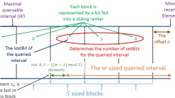 Figure 1
 Figure 2
 Figure 3
 Figure 4
 Figure 5
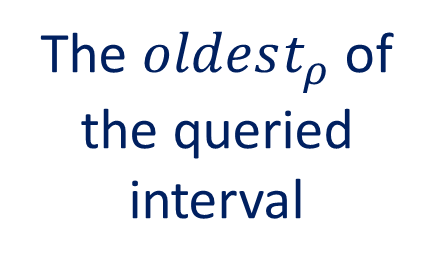 Figure 6
 Figure 7
 Figure 8
 Figure 9
 Figure 10
 Figure 11
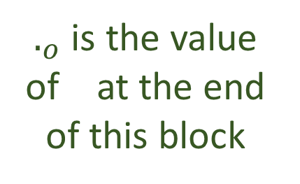 Figure 12
 Figure 13
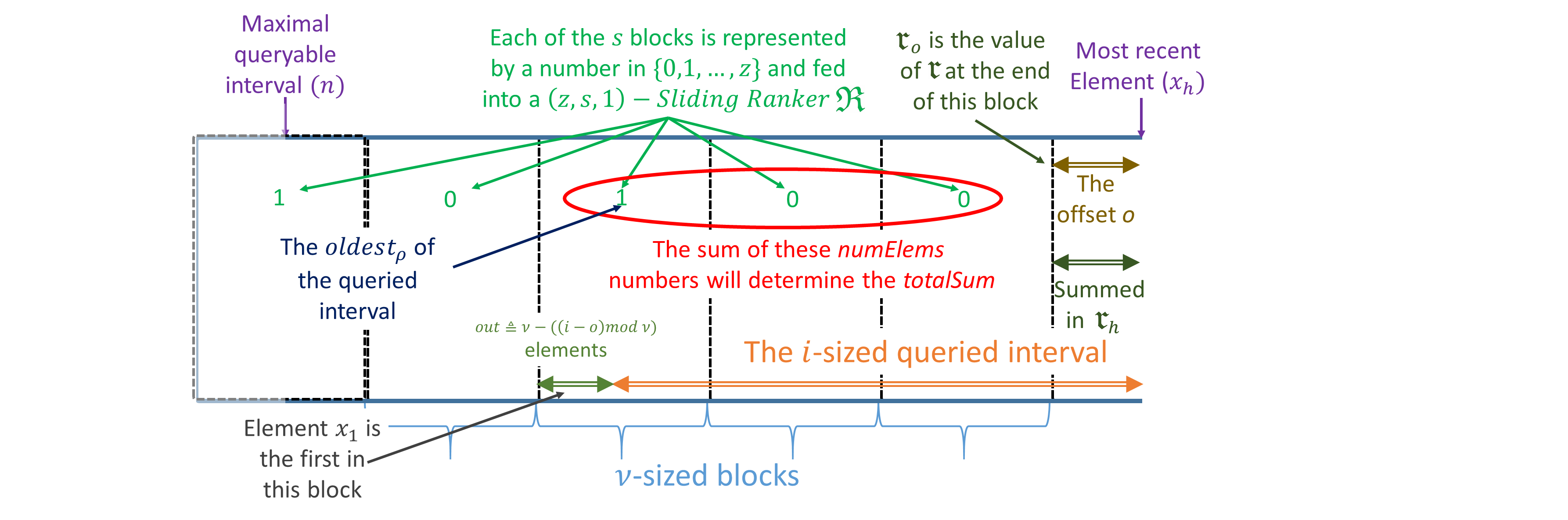 Figure 14
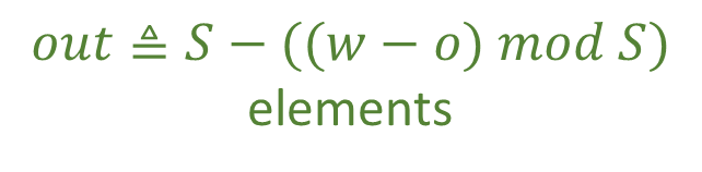 Figure 15
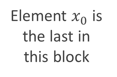 Figure 16
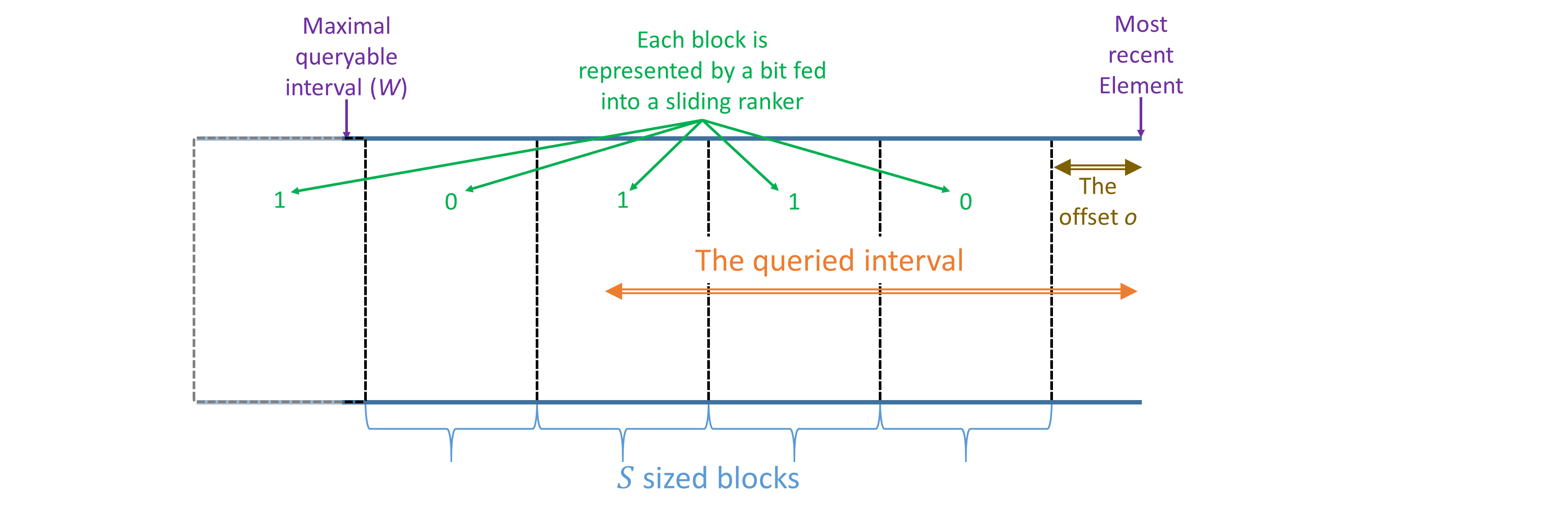 Figure 17
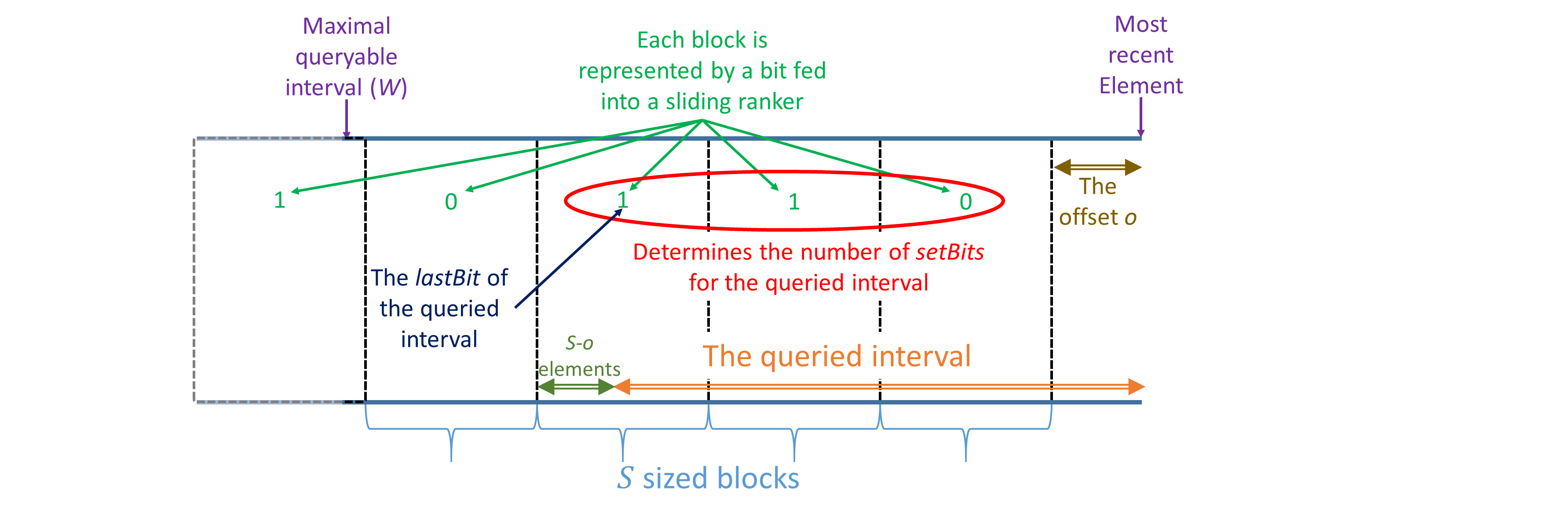 Figure 18
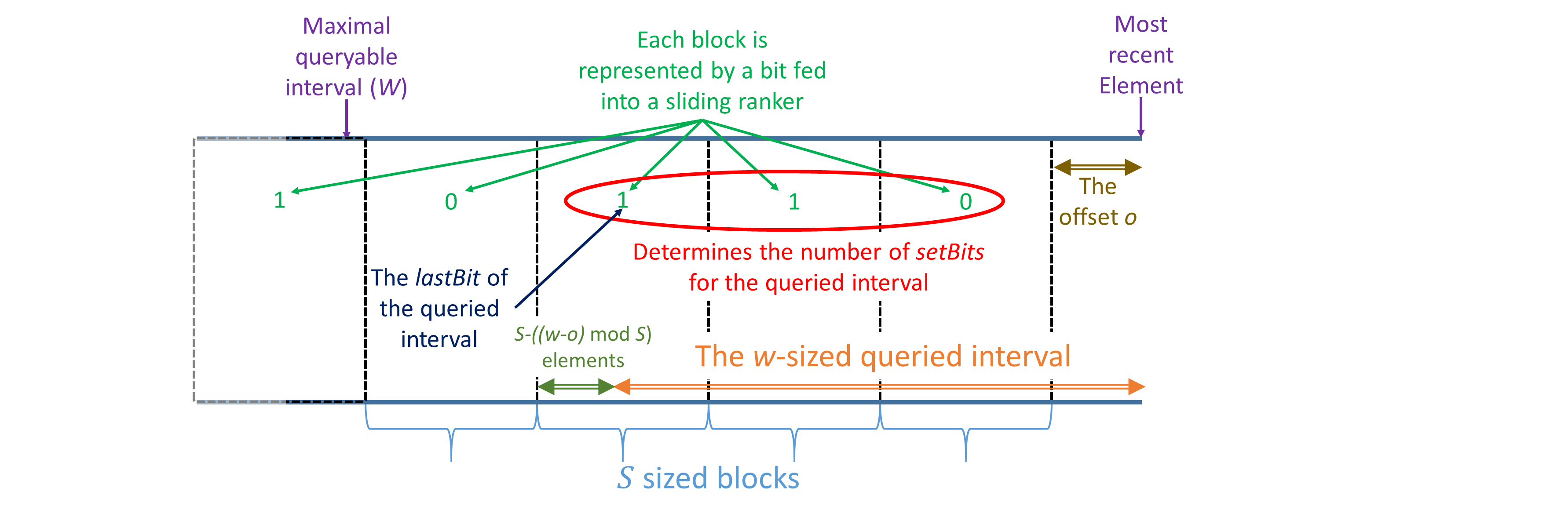 Figure 19
 Figure 20
 Figure 21
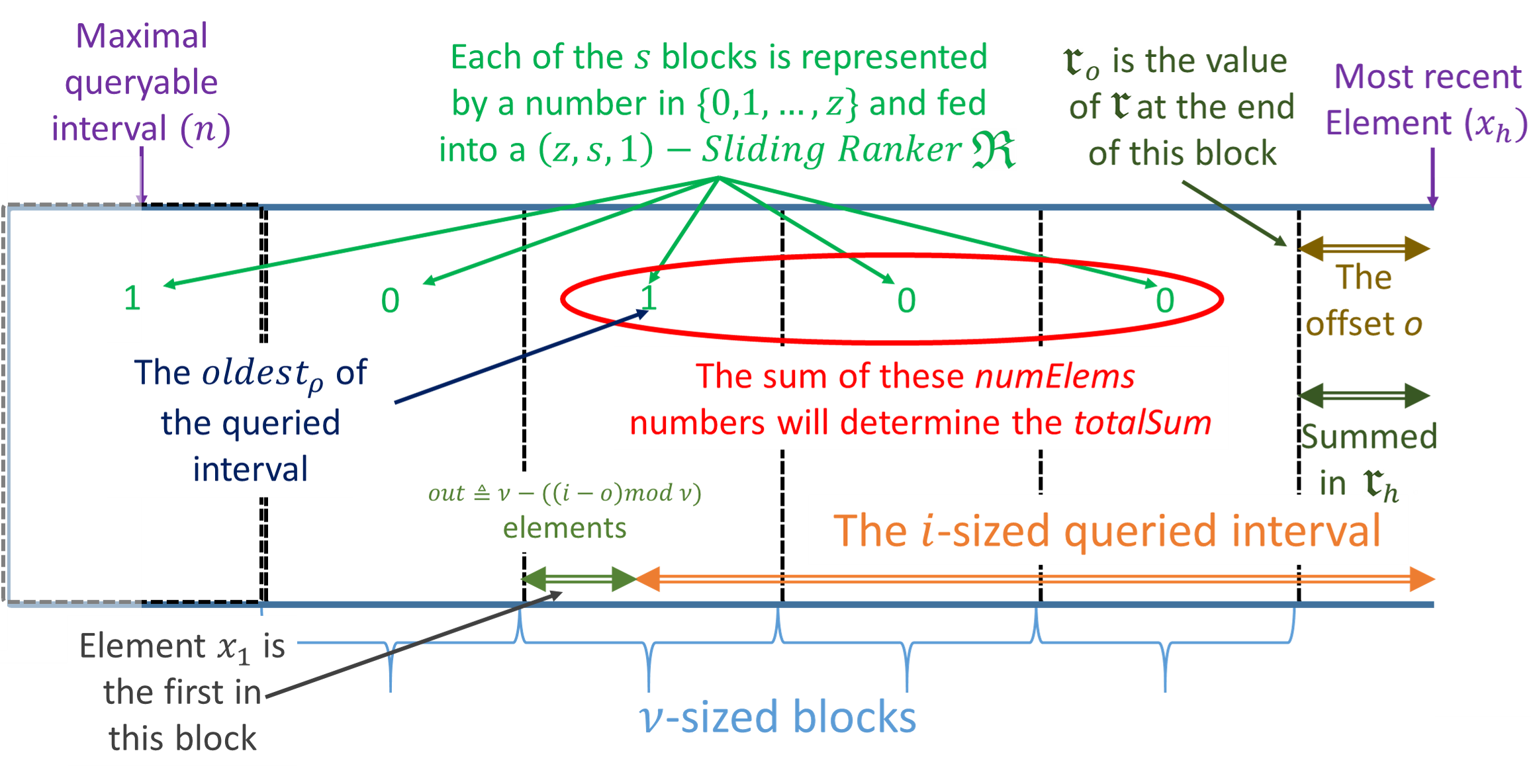 Figure 22
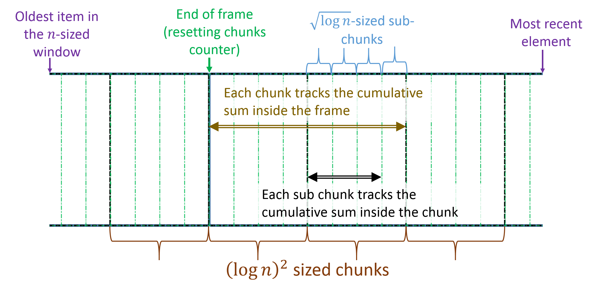 Figure 23
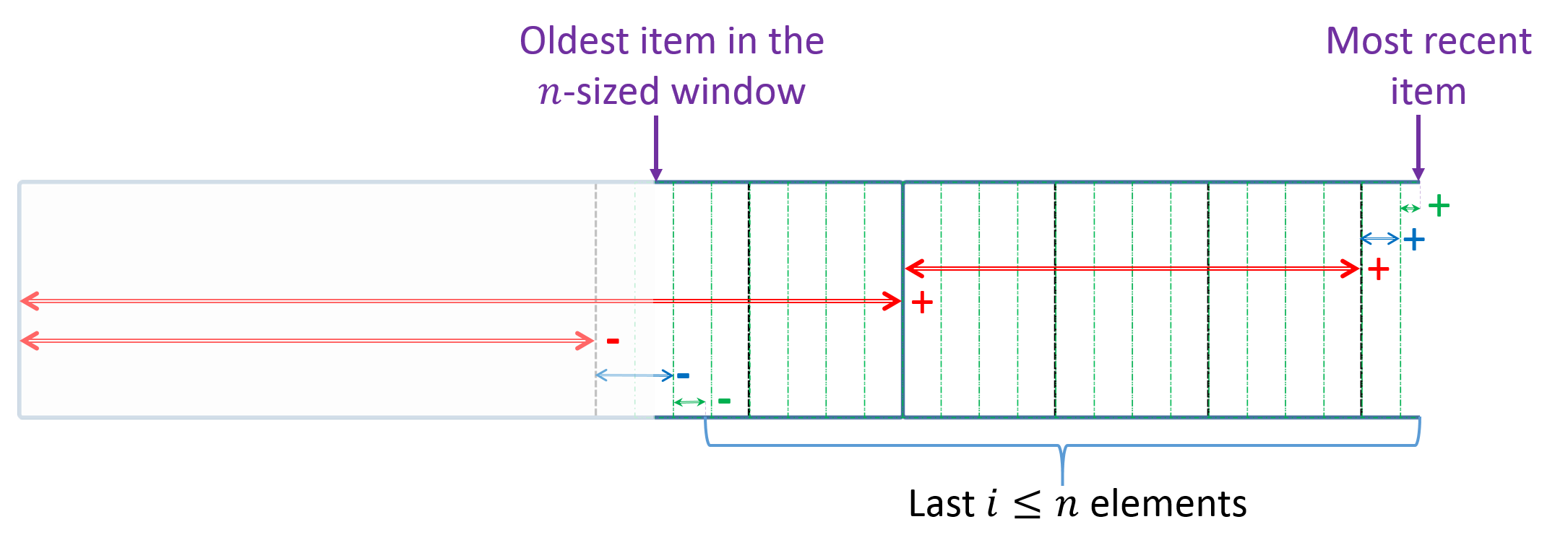 Figure 24
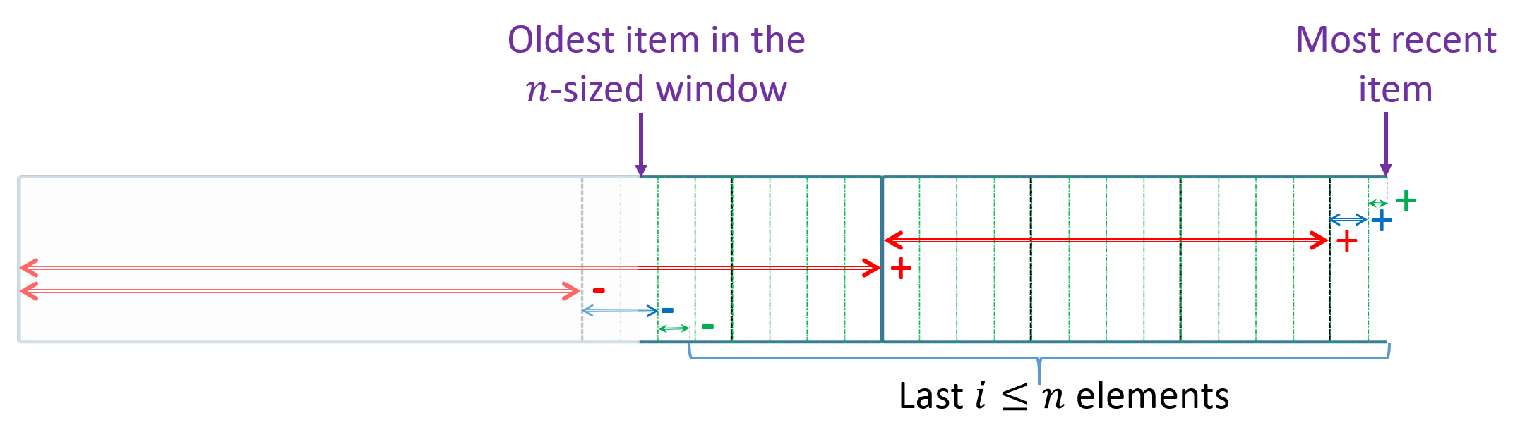 Figure 25
Peer Reviews
No public reviews on file for this paper yet. If you reviewed it on a platform where reviews are public (OpenReview, ICLR, NeurIPS, ICML), you can paste yours below so the community can read it here.
Videos
No videos yet. Explain this paper in a talk, walkthrough, or lecture? Add one.
Taxonomy
TopicsAlgorithms and Data Compression · Complexity and Algorithms in Graphs · Data Management and Algorithms
Succinct Approximate Rank Queries
Ran Ben Basat
Department of Computer Science
Technion
Abstract
We consider the problem of summarizing a multi set of elements in under the constraint that no element appears more than times. The goal is then to answer rank queries — given , how many elements in the multi set are smaller than ? — with an additive error of at most and in constant time. For this problem, we prove a lower bound of \mathcal{B}_{\ell,n,\Delta}\triangleq\left\lfloor{\frac{n}{\left\lceil{\Delta/\ell}\right\rceil}}\right\rfloor\log\big{(}{\max\left\{\left\lfloor{\ell/\Delta}\right\rfloor,1\right\}+1}\big{)} bits and provide a succinct construction that uses bits. Next, we generalize our data structure to support processing of a stream of integers in , where upon a query for some we provide a -additive approximation for the sum of the last elements. We show that this too can be done using bits and in constant time. This yields the first sub linear space algorithm that computes approximate sliding window sums in time, where the window size is given at the query time; additionally, it requires only more space than is needed for a fixed window size.
keywords:
Streaming, Network Measurements, Statistics, Lower Bounds
1 Introduction
1.1 Background
Static dictionaries are data structures that encode a set and efficiently answer membership queries of the form “is ?” (for some ). This problem was extensively studied and memory efficient data structures that allow time queries for it were suggested for several different models [6, 12, 20].
An extension of the dictionary problem is the Rank query, which given an identifier returns the number of elements in that are smaller than or equal to . For this problem as well, multiple papers proposed space efficient solutions with a constant query time [16, 21, 22]. The inverse problem, called Select query, asks for the ID of the smallest element in and was also shown to have space efficient data structures that support constant time queries [7, 21].
A seemingly different research area is the design of streaming algorithms. For many domains, such as networking, economics and databases, the ability to process large data streams is vital. As data varies over time, recent data is often considered more relevant; this motivated the study of sliding window algorithms, in which only the last elements are of interest. The sliding window model was studied for many problems such as summing [3, 10, 14]; counting the number of distinct elements [2, 13]; finding frequent elements [4, 15]; answering set membership queries [5, 17, 19]; and other problems [1, 9, 18, 23]. All these works share a common goal – they significantly reduce the memory consumption; in return, they settle for approximate, rather than exact, solutions. Given sufficient space, we can solve such problems exactly simply by adding the newly arriving item into our summary and deleting the element that has left the window. However, in many applications the window size is too large and the memory requirement becomes a major bottleneck. In this paper, we show how rank queries can be used for streaming.
Even if modern RAM memories seem to be enough for storing large element sequences, there are many advantages in minimizing the memory requirements. Routers, for example, often rely on the scarce SRAM which allows access at the speed in which they are required to route packets. If the measurement algorithms are not compact enough to fit into the small SRAM, they must access the slower DRAM that does not allow real time queries. This can be a significant limitation for applications that require timely insights about the traffic, such as load balancing or denial of service attack identification. Similarly, when implementing in software we can gain speed if we fit our algorithm into the CPU cache and reduce DRAM access. Smaller data structures might even fit in a single cache line and can be pinned there to maximize the measurement performance.
The works mentioned above significantly reduce the space requirements compared to storing the entire window in memory. However, these algorithms assume that the window size is known in advance and their data structures only allow queries about the predetermined window size to be answered efficiently. While we can maintain a different sketch for every window size that is of interest, this may be prohibitively expensive in terms of both memory and update time. Further, the goal of these algorithms is to enable memory feasible solutions to what would otherwise require storing the exact window in memory; thus, duplicating the data structures for multiple window sizes undermines the purpose for which they were created.
1.2 Our Contributions
Our first contribution is the extension of exact succinct rankers to multi sets in which every element can appear at most times. Previous works have considered multi sets under cardinality constraint for all elements combined. Here we address the natural case where every element may appear at most times, but no cardinality constraint (smaller than ) is known for the multi set. Our approach requires bits and allows time rank queries.
Our next contribution are novel approximate set and multi set representations that allow computing rank queries with an additive error of , while using less space than required for storing the multi set itself. For this problem, we prove a \mathcal{B}_{\ell,n,\Delta}=\left\lfloor{\frac{n}{\left\lceil{\Delta/\ell}\right\rceil}}\right\rfloor\log\big{(}{\max\left\{\left\lfloor{\ell/\Delta}\right\rfloor,1\right\}+1}\big{)} bits lower bound and a propose a succinct data structure that uses bits. To the best of our knowledge, this is the first algorithm that provides approximate rank queries in time using less memory than the set / multi set encoding requires.
Next, we extend the notion of approximate rankers to streams and propose algorithms that process a stream of integers in and answer sliding window sum queries in time. Unlike previous works [2, 3, 10], we get the window size at query time. That is, our algorithm can compute the sum of any window size while previous works assume that the size is fixed. Interestingly, our construction is succinct even when compared with the lower bound derived in [3] for fixed size windows. Thus, with a space overhead we allow the algorithm to support all window sizes. This is a major improvement over the naive approach of maintaining a separate algorithm instance for every window size that is of interest, in both space and time complexity.
We note that our approach also allows approximating the sum of historical intervals that can be used for drill-down queries. For example, assume that we are monitoring a 100Gbps link on a backbone router such that at each second we get the utilized bandwidth (i.e., we can set bits). Now, assume that we identify a distributed denial of service attack and want to study the link utilization pattern before and during the attack. Our algorithm allows us to estimate the bandwidth between any time interval (for ) simply by subtracting the estimate for the sum of the last seconds from the estimate of the last seconds’ sum.
2 Related Work
2.1 Dictionaries
Consider a set . A dictionary is a data structure that supports membership queries of the form “Is in ?”. Several hashing-based works proposed methods for efficiently encoding while supporting constant time membership queries [6, 12, 20, 24]. Dictionaries were then naturally extended to the Indexable Dictionary problem that also supports the operations:
Rank: given , return . 2. 2.
Select: given , return the smallest element in .
The problem of storing sets (and multisets, with the appropriate generalizations of the Rank and Select procedures) drew lots of attention from the research community [16, 21, 22]. Of special interest to us is the work of Jacobson [16] that allows constant time rank queries using memory. Jacobson’s idea was to look at the characteristic vector of the set, i.e., a bits vector whose entry is set if . Thus, the Rank query reduces to counting the number of set bits that precede some index given at query time. To achieve this, Jacobson breaks the vector into sized chunks. At the end of each chuck, Jacobson keeps the number of set bits that precede it. Since there are such chucks, and each is encoded using bits, this requires bits. Next, Jacobson focuses on each specific chunk and divides it into a sequence of -sized sub-chunks. At the end of each sub-chunk, Jacobson stores its number of preceding set bits within the current chunk using bits. Once again, the number of sub-chunks is so the total memory required is bits. Finally, Jacobson counts the number of set bits within each sub-chunk using a lookup table. In the table, the keys are all binary vectors of size at most and the values are the number of set bits; thus, the table’s overall memory consumption is .
In this paper, we present a succinct structure for rank queries of multi sets in which each element appears at most times. This is different than the multi set representations of [20, 21] that considered cardinality constraint for the entire multi set, but without any further restriction on the number of appearances of a single item. We also provide an encoding that supports additive approximations of rank queries in less memory than required for encoding the multi set.
2.2 Algorithms that Sum over Sliding Windows
Approximating the sum of the last elements over an integer stream, known as Basic-Summing, was first introduced by Datar et al. [10]. They assumed that each element is in and proposed a multiplicative approximation algorithm. Their data structure, named Exponential Histogram , is based on keeping timestamps of element sequences called buckets such that the last elements fit into buckets. Each bucket requires bits to store the timestamp in addition to bits to store the bucket size. Overall, the number of bits required by their algorithm is and it operates in amortized time or worst case. The EH approach was then extended in [1] for other statistics over sliding windows, such as median and variance. In [14], Gibbons and Tirthapura presented a multiplicative algorithm that operates in constant worst case time while using similar space for . In [3], we studied the potential memory savings one can get by replacing the multiplicative guarantee with a additive approximation. We showed that bits are required and sufficient.
In a sliding window, the last elements get similar weight while older items do not affect the sum. Cohen and Strauss [8] considered more general aging models where older data has lower weight, but the rate in which the weight decreases may be different than that of sliding windows.
Recently, we studied [2] the affect that allowing an error in the window size has on the required memory of approximate summing algorithms. Specifically, we showed that if upon a query the algorithm is required to return a tuple such that and then bits are needed.
All of the algorithms above assume that the window size is fixed. Here, we propose solutions that are succinct, even when compared to a lower bound derived here for static data, or to the bound for a fixed size window as in [3].
It is worth mentioning that these data structures do allow computing the sum of a window whose size is given at the query time. Alas, the query time will be slower as they do not keep aggregates that allow quick computation. Specifically, we can compute a multiplicative approximation using a slightly extended version of EH [11] in time by a binary search for the block with the right timestamp. We can also use the data structure of [3] for an additive approximation of in time, and utilize [2]’s structure for a -approximation in time . In this paper we offer solutions that operate in time.
3 Preliminaries
We say that an algorithm is succinct if it uses bits, where is the information-theoretic lower bound for the problem it solves. Throughout the paper, we assume the standard word RAM model with a word size of . For simplicity of presentation, we also assume that and are integers.
Definition 3.1** (Approximation).**
Given a value and a constant , we say that is an -additive approximation of if .111We use one-sided error, and strict inequality as this simplifies our computations.
Next, we define the notion of an -Ranker – a structure that can answer approximate rank queries in a memory efficient manner. Specifically, -Ranker is a succinct encoding of a multi-set over such that no element appears more than times, that supports time rank queries.
Definition 3.2** (Static Ranker).**
An -Ranker, for some , is an algorithm that preprocesses a sequence in and when queried with some returns a -additive approximation of the sum of the first elements, , in time.
We proceed with the definition of a Sliding Ranker, extending -Rankers to streams, while focusing on the last elements in the stream for supporting sliding window queries.
Definition 3.3** (Sliding Ranker).**
*An -Sliding Ranker, for some , is an algorithm that processes a stream of integers in and when queried for some returns a -additive approximation of the last elements sum, , in time. *
4 -Rankers
In order to construct an -Ranker, we first discuss the special case of zero-error ().
4.1 An -Ranker
Here, we provide a succinct construction of -Ranker, for any . Intuitively, this generalizes Jacobson’s ranker [16] that addresses binary sequences (). As we show, his lookup table approach works for “small” values of . In other cases, such as , we can split the vector into smaller and smaller intervals (i.e., sub-sub-chunk, etc.), but if the number of levels is constant, storing a lookup table for the smallest level is infeasible in space. Thus, we use a different trick for large values for computing within-sub-chunk sums in . We avoid keeping the and the characteristic vector; instead, we keep a -sized array in which each entry contains the sum of the sub-chunk up to that point. For example, if the sub-chunk was , we store regardless of vector entries outside this sub-chunk. Since is “large”, this takes space.
We start by noting that since the number of sequences in is , any algorithm that computes such rank queries (exactly) requires bits. We also note that without a query time constraint this is achievable, as we can simply store the entire data and when queried sum the required interval in time. Thus, if (i.e., we have a small array of potentially large numbers), then the same idea works and we therefore require bits; hence, we hereafter assume that . Next, we will prove the following:
Theorem 4.1**.**
For any , there exists an -Ranker that uses bits.
We start by breaking the sequence into chunks of size , keeping the cumulative sums at the end of each chunk. The required number of bits for these sums is at most
[TABLE]
where the last equation follows from .
Next, we break the chunks into sub-chunks of size and keep the cumulative sum from the beginning of the most recent chunk at the each sub-chunk’s end. The memory consumption of these sub-chunk aggregates is then no more than
[TABLE]
We are left with the task of efficiently computing the sub-chunk sums. Here, we split our construction depending on the relation between and .
- •
.
In this case, we adopt Jacobson’s lookup table approach. Specifically, we create a lookup table ; the key of each table entry is a -sized sequence of elements in and an index . Its value is the sum of the first sequence entries. In order to use the table, we also store the characteristic vector itself using bits. The size of the table is then
[TABLE]
Thus our overall memory consumption is . Unfortunately, while we can consider smaller and smaller sequence aggregates, constructing such a lookup table will prevent the algorithm from being succinct when is large (e.g., for ).
- •
.
In this case, we return to the cumulative approach. Instead of storing the characteristic vector (and without a lookup table) we store for each element the cumulative sum from the beginning of its sub-chunk. Since the sub-chunks are of size , the number of bits this takes is
[TABLE]
We conclude that in all cases our construction requires bits and is thus succinct.
4.2 An -Ranker for
We start by proving a lower bound on the memory required by any -Ranker. For convenience, we denote . We only consider , as means zero-error and allows the algorithm to always return [math], regardless of the input.
Theorem 4.2**.**
Let , then the number of bits required by any deterministic -Ranker is at least
[TABLE]
Proof 4.3**.**
We denote and . Next, consider all inputs that contain a sequence of blocks padded by zeros, such that each block is a member of ; that is, consider . Notice that each literal is in the range and that each input is of size as required. We show that every two inputs in must lead to distinct configurations in the -Ranker, thereby implying a bits lower bound as required. Let be two distinct inputs in such that for any . Denote by the first block’s index in which differs from . Now consider a query for . If , then and (due to the definition of ) , which implies an error of at least for at least one of the inputs. On the other hand, means that and thus either or . In either case, the difference in sums is at least . We established that if two inputs in lead to the same configuration, the error for one of them would be at least while we assumed it is strictly lower.
We now present a succinct construction of an -Ranker. Denote and . For creating an -Ranker, we first show how to “compress” the input into a smaller problem that we solve exactly. Intuitively, we create a new -long input , such that each of its elements is bounded by , and then employ a -Ranker, . Alas, if , this is not enough to allow succinct encoding; for this, we also compute the fraction of the input’s sum that is not accounted for in and use it for answering queries. Given an input , we create iteratively as follows222If , we implicitly define and :
[TABLE]
Then, we compute the remainder:
[TABLE]
After computing , we feed it into a -Ranker denoted . Given a query for some , we returnfootnote 2
[TABLE]
which we can compute in as follows: 333We note that if our ranker was originally constructed to compute the sum of the last elements rather than the first, only two queries were needed.
[TABLE]
Lemma 4.4**.**
[TABLE]
Proof 4.5**.**
We denote the error in the representation of the last items by
[TABLE]
Observe that and hence
[TABLE]
Next, we use (1) to obtain
[TABLE]
We now perform a case analysis, based on the value of and start with the simpler case where . In this case, we have and thus we can rearrange (4) as:
[TABLE]
and using (3) we immediately get .
Next, we focus on the case of . Thus, we hereafter have and . We now consider if and when both and (which implies ); observe that
[TABLE]
Thus, if , then
[TABLE]
Next, we split to cases based on the value of :
- •
. In this case, according to (4) and (5) we have:
[TABLE]
On the other hand, we bound the error from above as follows:
[TABLE]
- •
. Similarly to before, using (4) and (5) we get:
[TABLE]
Now, we use the fact that both and are integers to deduce that . Finally, we bound the error from above:
[TABLE]
We conclude that in all cases we have .
Next, we show that the value of each entry in is smaller than , as stated.
Lemma 4.6**.**
For any , .
Proof 4.7**.**
Notice that . For other values, we have
[TABLE]
We now bound for analyzing the space of our construction; the proof appears in Appendix A.
Lemma 4.8**.**
For any input , the remainder in (1) satisfies .
Follows is an analysis of our ranker.
Lemma 4.9**.**
Let and . The number of bits required by our ranker is (1+o(1))\cdot\left\lfloor{n/\max\left\{\left\lfloor{\mu}\right\rfloor,1\right\}}\right\rfloor\cdot\log\big{(}{\left\lceil{\mu^{-1}}\right\rceil+1}\big{)}.
Proof 4.10**.**
Our construction has two components: the exact ranker and the remainder . As is a -Ranker, where and , it requires bits according to Theorem 4.1. Recalling that gives us the desired bound. Finally, Lemma 4.8 tells us that and can therefore be represented using bits.
Theorem 4.11**.**
Let such that , the construction above is an -Ranker that uses bits.444In other cases, our construction uses at most bits but might not be succinct.
Proof 4.12**.**
Recall that \mathcal{B}_{\ell,n,\Delta}=\left\lfloor{n/\left\lceil{\mu}\right\rceil}\right\rfloor\log\big{(}{\max\left\{\left\lfloor{\mu^{-1}}\right\rfloor,1\right\}+1}\big{)} while our algorithm uses (1+o(1))\cdot\left\lfloor{n/\max\left\{\left\lfloor{\mu}\right\rfloor,1\right\}}\right\rfloor\cdot\log\big{(}{\left\lceil{\mu^{-1}}\right\rceil+1}\big{)} bits. If , we have \mathcal{B}_{\ell,n,\Delta}=n\log\big{(}{\left\lfloor{\mu^{-1}}\right\rfloor+1}\big{)}=(1-o(1))n\log\mu^{-1} when our structure takes (1+o(1))\cdot n\cdot\log\big{(}{\left\lceil{\mu^{-1}}\right\rceil+1}\big{)}=(1+o(1))n\log\mu^{-1} bits. Similarly, if then while we require . The case for follows from similar arguments.
5 -Sliding Rankers
As in the case of static data rankers, we first consider the exact case where .
5.1 An -Sliding Ranker
In this section, we provide a construction for an -Sliding Ranker that requires bits, where is the information-theoretic lower bound even without considering sliding windows. Intuitively, we adapt our -Ranker construction to the sliding window setting by incrementally building the chunks and sub-chunks. We start by breaking the stream into -sized frames. As in the original construction, we split the frames into sized chunks, where each chunk is further divided into -sized sub-chunks. In the case where , we keep a sized lookup table that maps each sequence in to its sum. If , we simply track the sums within a sub-chunk by keeping the cumulative sum for each item. We keep the chunk aggregates in a -sized circular buffer, and the sub-chunk aggregates in a similar structure of size . Finally, we “reset” the frame accumulator every elements, so that each chunk’s aggregate is always smaller than . Since each of the chunk aggregates requires bits and each of the sub-chunk aggregates takes bits, our overall space consumption is as required. Our -Sliding Ranker construction is illustrated in Figure 1, while the query procedure is exemplified in Figure 2. In Appendix D we provide an algorithm for the case; here, we hereafter assume that .
Our algorithm uses the following variables:
- •
- a cyclic buffer of integers, each allocated with bits.
- •
- a cyclic buffer of integers, each allocated with bits.
- •
- the sum of elements inside the current frame.
- •
- the index of the most recent item, modulo .
- •
- a lookup table mapping sequences of length to their sums.
- •
- the last elements window.
We give a pseudo code of our -Sliding Ranker in Algorithm 1.
We now formulate the properties of the algorithm; the theorem’s proof is deferred to Appendix B due to lack of space.
Theorem 5.1**.**
Algorithm 1 is an -Sliding Ranker that uses memory bits.
5.2 An -Sliding Ranker for
Similarly to the way we used -Rankers to construct -Rankers for any , we now use the exact -Sliding Ranker for constructing an -Sliding Ranker.
Intuitively, we split the stream into blocks of size and construct the remainder gradually; whenever a block ends, we compute a new value and feed it into an exact we use as a black box. When queried, we employ our exact ranker and remainder to estimate the relevant sum, similarly to our -Ranker queries from Section 4.2. However, if we simply sum the elements using , it will require bits; this will not allow us to remain succinct if as the lower bound for this case is and is independent of (given that is fixed). To solve this, we follow [3]’s approach and round every arriving element, representing it using bits. That is, if arrived, we consider instead. To compensate for the rounding error, we will need blocks of size smaller than that we used in our -Ranker construction; specifically, we set . Additionally, when the block size has to remain , so we have to compensate for the rounding error by other means; this is achieved by reducing the “sensitivity” to .555If , then we simply apply the exact algorithm from the previous subsection. The parameters for the exact ranker are then and . Our algorithm uses the following variables:
- •
- a , as described in Section 5.1.
- •
- tracks the sum of elements that is not yet recorded in .
- •
- the offset within the block.
A pseudo code of our method appears in Algorithm 2.
Next follows a memory analysis of the algorithm with a proof given in Appendix C.
Lemma 5.2**.**
Algorithm 2 requires (1+o(1))\cdot\left\lfloor{n/\max\left\{\left\lfloor{\mu}\right\rfloor,1\right\}}\right\rfloor\cdot\log\big{(}{\left\lceil{\mu^{-1}}\right\rceil+1}\big{)}+O\left({\log n}\right) bits.
This allows us to conclude, similarly to Theorem 4.11, that our algorithm is succinct if the error satisfies . We also note that a lower bound was shown in [3] even when only fixed sized windows (where ) are considered. Thus, our algorithm always requires at most , even if the allowed error is .
Corollary 5.3**.**
Let such that satisfies
[TABLE]
then Algorithm 2 is succinct. For other parameters, it uses space.
The following theorem, whose proof is deferred to Appendix E due to lack of space, shows the correctness of the algorithm.
Theorem 5.4**.**
Algorithm 2 is an -Sliding Ranker.
6 Discussion
In this paper, we studied the properties of data structures that support approximate rank queries for multi sets in which each element in appears at most times. We showed a lower bound for the problem and succinct constructions that require times as much memory. We then extended our approach and provided algorithms that process data streams and handle sliding window sum queries. Unlike previous work, we do not assume that the window size is fixed but rather get it at the query time. Interestingly, we show that this is doable in constant time and an additional space factor.
In the future, we would like to study structures that allow approximate select queries in time. This will allow efficient approximate-percentile computation for multi sets. We note that this is already achievable with our data structure in time using a binary search over the rank queries. We also plan to explore the possibility of creating approximate rankers with a multiplicative error rather than additive. Finally, we wish to extend our approach to problems other than summing; e.g., computing heavy hitters for a sliding window whose size is given at the query time.
Appendix A Proof of Lemma 4.8
Proof A.1**.**
[TABLE]
If , then and thus . Otherwise, we have .
Appendix B Proof of Theorem 5.1
We start with analyzing the memory requirements of our algorithm.
Lemma B.1**.**
Algorithm 1 uses memory bits.
Proof B.2**.**
We have chunks, each represented using bits. Similarly, each of the sub-chunk aggregates requires bits as its value is bounded by . Our window, uses bits, while the and variables require bits. Thus, the overall space consumption is .
We are now ready to prove the theorem.
Proof B.3**.**
Denote the stream by , such that the most recent element’s index is , where is the offset within the current frame and frames were completed so far. We assume that . The case for follows from similar arguments. We start with a few straight forward observations. Notice that always contains the sum of the last frame that was completed; that is, . Next, for any positive , we have that contains the sum of the last -indexed chunk that was completed, i.e.,
[TABLE]
Similarly, we have that :
[TABLE]
Given a query for , the goal of an -Sliding Ranker is to return the quantity . First, we express the sum of elements from the beginning of the previous frame, , as:
[TABLE]
Next, since , we have that
. 2. 2.
. 3. 3.
. 4. 4.
.
Notice that if , these are the first four summands of Line 18; if , then we do not add to the sum. In both cases, we are left with the need to subtract the sum of elements, starting from the beginning of the relevant frame, that are not a part of the last items. Similarly to the above, we have that the sum from the beginning of the previous frame to the newest item is: . If the last items are all contained in the current frame (i.e., ), then we have:
[TABLE]
In this case, we get:
. 2. 2.
. 3. 3.
. 4. 4.
.
Here, we cancel the effect of simply by not adding it as one of the summands (the If condition of Line 16). Quantities 2,3 and 4 are the three subtrahends of our query procedure. Finally, if we do add the value of , and thus in all cases we successfully compute the sum of the last elements.
Appendix C Proof of Lemma 5.2
Proof C.1**.**
The algorithm utilizes three variables: that requires , that uses bits, and is allocated with bits. Overall, the number of bits used by our construction is
[TABLE]
*Since , we get the desired bound. *
Appendix D An -Sliding Ranker for
Here, we detail the construction for the case of large value. We do the same splitting into frames, chunks, and sub-chunks as before. However, the large value of does not allow us to succinctly store the lookup table as before. Instead, we keep for each element the sum from the beginning of its sub-chunk, similarly to our solution in Theorem 4.1. Our algorithm uses the following variables:
- •
- a cyclic buffer of integers, each allocated with bits.
- •
- a cyclic buffer of integers, each allocated with bits.
- •
- the sum of elements in the current frame.
- •
- the sum of elements in the current sub-chunk.
- •
- the most recent element’s index, modulo .
- •
- a cyclic array that contains for each item the sum from the beginning of its sub-chunk.
We give a pseudo code of our -Sliding Ranker in Algorithm 3. Next, we analyze the properties of the algorithm.
Theorem D.1**.**
Algorithm 3 uses memory bits for .
Proof D.2**.**
Similarly to the analysis in Lemma B.1, the algorithm uses bits for keeping the chunk and sub-chunk aggregates. Here, we replaced the lookup table and the array of window elements by an array that stores the within-sub-chunk cumulative sum for each element. That is, each entry in the -sized array stores a number in and thus the array requires bits overall.
Theorem D.3**.**
Algorithm 3 is an -Sliding Ranker.
Proof D.4**.**
*Observe that the query procedure of our algorithm is equivalent to that of Algorithm 1, except for the part where it uses the lookup table. We now use the variable to compute the sum of the current sub-chunk instead of looking it up in the table. The sum of elements that preceded the last items in ’s sub-chunk is then retrieved from . As we simply track the sum of items prior to that index in and then store it in (see line 5), we get its value immediately. Thus, our estimation procedure is equivalent to that of Algorithm 1 and using Theorem 5.1 we establish our correctness. *
Appendix E Proof of Theorem 5.4
Proof E.1**.**
For the proof, we define a few quantities that we also use in our query procedure and as in our Query function; see Figure 3 for illustration. We assume that the index of the most recent element is
[TABLE]
such that is the offset within the current block and that is the first element in the newest block of . By the correctness of the Sliding Ranker, and as illustrated in Figure 3, we have that is the sum of the last added to , that is the value of the element that represents the last block that overlaps with the queried window. Also notice that is the number of elements in that block that are not a part of the window.
For any , we denote by the value of after the item was added; e.g., is the value of at the time of the query and is its value after the last block has ended. For other variables, we consider their value at the query time.
When a block ends, we effectively perform (lines 6 and 7) and thus:
[TABLE]
Our goal is to estimate the quantity
[TABLE]
Recall that our estimation (Line 17) is:
[TABLE]
where the last equality follows from the fact that within a block we simply sum the rounded values (Line 4). Next, observe that we sum the rounded values in each block and that if is decreased by (for some ) in Line 7, then we set one of the last elements added to to . This means that:
[TABLE]
Plugging (9) into (8) gives us
[TABLE]
Joining (10) with (7), we can express the algorithm’s error as:
[TABLE]
where is the rounding error which is defined as
[TABLE]
Since each rounding of an integer has an error of at most , and as we round elements, we have that the rounding error satisfies
[TABLE]
where the last inequality is immediate from our choice of the number of bits that is . We now split to cases based on the value of . As in the -Ranker case, we start with the simpler case, in which (and consequently, ). This allows us to write the algorithm’s error of (11) as
[TABLE]
We now use (6),(12) and the definition of to obtain:
[TABLE]
Similarly, we can bound it from below:
[TABLE]
We established that if we obtain the desired approximation. Henceforth, we focus on the case where , and thus and . We now consider two cases, based on the value of .
** case.
In this case, we know that after the processing of element the value of was at least (Line 6). This implies that and equivalently*
[TABLE]
Substituting this in (11), and applying (12), we get that:
[TABLE]
In order to bound the error from above we use (6) and (12):
[TABLE] 2. 2.
** case.
*** Here, since the value of was is [math], we have that and thus*
[TABLE]
We use this for the error expression of (11) to get:
[TABLE]
We now use (6), (12), and the fact that to bound the error from below as follows:
[TABLE]
Finally, we need to cover the case of . In this case, we return as the estimate. This directly follows from (6) and the fact that within a block we simply sum the rounded values (Line 4). We established that in all cases , thereby proving the theorem.
The reference list from the paper itself. Each links out to its DOI / PubMed record.
- 1[1] Brian Babcock, Mayur Datar, Rajeev Motwani, and Liadan O’Callaghan. Maintaining variance and k-medians over data stream windows. In ACM PODS , 2003.
- 2[2] Ran Ben Basat, Gil Einziger, and Roy Friedman. Efficient network measurements through approximated windows. Co RR:1703.01166 .
- 3[3] Ran Ben Basat, Gil Einziger, Roy Friedman, and Yaron Kassner. Efficient Summing over Sliding Windows. In SWAT , 2016.
- 4[4] Ran Ben-Basat, Gil Einziger, Roy Friedman, and Yaron Kassner. Heavy hitters in streams and sliding windows. In IEEE INFOCOM , 2016.
- 5[5] Ran Ben-Basat, Gil Einziger, Roy Friedman, and Yaron Kassner. Poster abstract: A sliding counting bloom filter. In IEEE INFOCOM , 2017.
- 6[6] Andrej Brodnik and J Ian Munro. Membership in constant time and almost-minimum space. SIAM Journal on Computing , 28(5):1627–1640, 1999.
- 7[7] David Clark. Compact Pat trees . Ph D thesis, Ph D thesis, University of Waterloo, 1998.
- 8[8] Edith Cohen and Martin J. Strauss. Maintaining time-decaying stream aggregates. Journal of algorithms , 59(1):19–36, 2006.