
TL;DR
This paper characterizes the lattice structure of ground spaces of hermitian matrices, revealing their geometric properties and connections to quantum marginals and local Hamiltonians.
Contribution
It introduces a novel characterization of lattice elements and maximal elements of ground spaces using operator cone constraints, advancing the understanding of quantum marginal geometry.
Findings
Lattice elements of ground spaces are characterized by operator cone constraints.
Maximal lattice elements correspond to specific subspace structures.
Results link ground space lattices to quantum marginal face lattices.
Abstract
The ground spaces of a vector space of hermitian matrices, partially ordered by inclusion, form a lattice constructible from top to bottom in terms of intersections of maximal ground spaces. In this paper we characterize the lattice elements and the maximal lattice elements within the set of all subspaces using constraints on operator cones. Our results contribute to the geometry of quantum marginals, as their lattices of exposed faces are isomorphic to the lattices of ground spaces of local Hamiltonians.
Click any figure to enlarge with its caption.
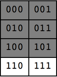 Figure 1
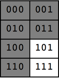 Figure 2
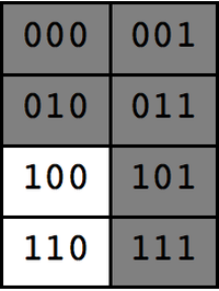 Figure 3
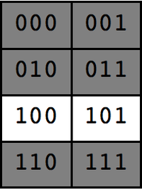 Figure 4
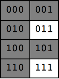 Figure 5
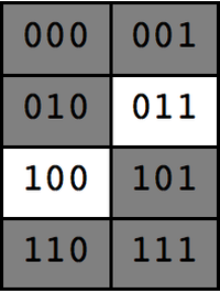 Figure 6
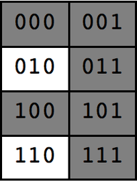 Figure 7
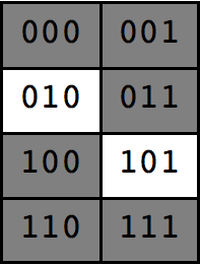 Figure 8
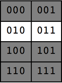 Figure 9
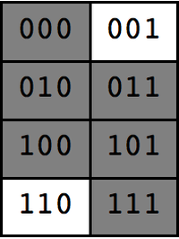 Figure 10
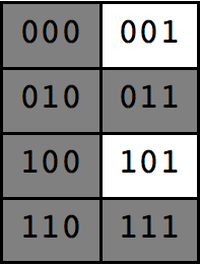 Figure 11
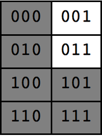 Figure 12
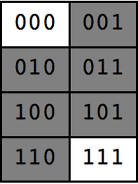 Figure 13
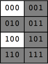 Figure 14
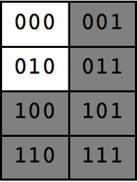 Figure 15
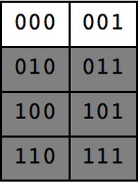 Figure 16
 Figure 17
Peer Reviews
No public reviews on file for this paper yet. If you reviewed it on a platform where reviews are public (OpenReview, ICLR, NeurIPS, ICML), you can paste yours below so the community can read it here.
Videos
No videos yet. Explain this paper in a talk, walkthrough, or lecture? Add one.
A variation principle for ground spaces
Stephan Weis
Abstract.
The ground spaces of a vector space of hermitian matrices, partially ordered by inclusion, form a lattice constructible from top to bottom in terms of intersections of maximal ground spaces. In this paper we characterize the lattice elements and the maximal lattice elements within the set of all subspaces using constraints on operator cones. Our results contribute to the geometry of quantum marginals, as their lattices of exposed faces are isomorphic to the lattices of ground spaces of local Hamiltonians.
Key words and phrases:
convex set, exposed face, normal cone, variation principle, quantum marginals, local Hamiltonian, ground space, operator cone, coatom.
2010 Mathematics Subject Classification:
Primary 52A20, 52B05, 51D25, 47L07, 47A12, 81P16. Secondary 62F30, 94A17.
\markleft
A variation principle for ground spaces
1. Introduction
The variation principle [27, 51] for estimating the ground energy (smallest eigenvalue) of a Hamiltonian (hermitian matrix) asserts that
[TABLE]
for all pure states . This means that is the smallest expected energy a quantum system can have in any pure state if is the energy operator. The upper bound on is mathematically trivial but computationally very useful. Nevertheless, the estimation of for the class of -local Hamiltonians, describing the energy of a many-body system without interactions between more than units, is a hard problem already for [36, 35, 20]. Geometric approaches to the local Hamiltonian problem of estimating are discussed since the 1960’s. A basic idea is that is the displacement of the supporting hyperplane with normal vector touching the convex set of -body marginals.
Similar to the local Hamiltonian problem, the quantum marginal problem of deciding whether a tuple of states lies in is neither believed to have efficiently computable solutions [39, 60]. Many of the results pertaining to were originally obtained in the fermionic case (not treated here). Notably, spectral properties of marginal density matrices [19, 3, 52, 18] were discovered. Spectral conditions are insufficient to characterize -body marginals of overlapping subsystems (), for that there are results concerning extreme points [19, 23, 45, 17] and order-theoretic results regarding ground spaces of marginal states [16].
In this article we study order-theoretic aspects of the convex geometry of a set of quantum marginals—we begin with linear images of general convex sets, then linear images of state spaces of matrix algebras, and finally the very special case of quantum marginals . More precisely, a quantum mechanical system [15, 2] is described by a complex *-subalgebra of including the -by- identity matrix . A density matrix, or state, of is a matrix of trace one in the cone of positive semi-definite matrices in . The states of form a convex set , called state space.
According to the variation principle (1.1) and using a simple convexity argument, the ground energy of a Hamiltonian is
[TABLE]
where is the Hilbert-Schmidt inner product of . Assuming lies in a linear subspace of hermitian matrices, Euclidean geometry shows
[TABLE]
where is the orthogonal projection onto . Geometrically, equation (1.2) means that the ground energy restricted to is the distance of the origin from the supporting hyperplane of with inner normal vector .
A well-known aspect of is the isomorphism between its exposed faces and the ground projections of . An exposed face of is the intersection of with a supporting hyperplane, that is the subset of at which the minimum (1.2) is achieved for some . The ground projection of is the spectral projection of corresponding to the smallest eigenvalue. The ground space of is the image of . The set of exposed faces of , partially ordered by inclusion, is lattice-isomorphic to the set of ground projections of , partially ordered by the Löwner partial ordering [57].
A discussion of normal cones of leads to the Definition 5.2 of the cone
[TABLE]
for projections , that is . Thereby, is the complementary projection of , and . Notice that
[TABLE]
where is the kernel projection of . It is easy to show that if , then the ground projection of any is greater than or equal to any projection satisfying . Theorem 5.4 completes this statement to what we call variation principle: For every projection , the set of projections satisfying has a greatest element and .
The variation principle shows that the decision problem of whether a projection lies in is equivalent to that of whether . One way to compute is to pick a relative interior point of and compute its ground projection , as follows from results concerning normal cones of state spaces [54]. This raises the question, not teated here, of whether a relative interior point of can be efficiently computed.
The computation of can be put down to that of the maximal elements of , known as coatoms, as the latter generate in terms of infima [57]. Clearly, a projection of of rank is a coatom if and only if , that is if is a ray. Theorem 6.1(1) proves for any that is a coatom if and only if is a ray. The interesting part of the theorem, that is not a coatom if , is exploited in Section 8. Infima of projections are studied, for example, in [37, 26, 14].
The article is organized as follows. Section 2 proves a variation principle for convex sets. Sections 3 and 4 recall lattice isomorphisms related to the state space and its linear images. Section 5 translates the variation principle to ground spaces. Section 6 characterizes coatoms. Section 7 discusses a non-commutative example. Sections 8 and 9 deal with local Hamiltonians. Section 10 is a conclusion.
Remark 1.1** (Complexity of ).**
The semi-definite extension complexity [24, 5] of is the minimal dimension for which is a linear image of an affine section of . The local Hamiltonian problem being hard for , the existence of efficient algorithms [43] for linear optimization on suggests that the complexity of for qubits is unlikely to be polynomial in . Because of the gap from to the polynomial , the set has a much richer convex geometry than sections and projections of can have for of order .
Remark 1.2** (Topology of ).**
In addition to contributing to the geometry of , we hope that the results will ultimately enable us to discuss the topology of . If the algebra is non-commutative, then may not be closed in the norm topology, because of discontinuities of the maximum-entropy inference map under linear constraints [58]. For example, is not norm closed for three qubits [50]. For a many-body system, the discontinuity of the inference map is equivalent [56, 59, 50] to that of a correlation quantity [4, 7, 61, 6, 48, 44, 30] closely related to the “irreducible correlation” first introduced in [38]. For , the quantity is the mutual information or multi-information, which is continuous and which measures the total correlation [28].
2. A variation principle for pre-images of exposed faces
We show that the pre-images of exposed faces of a projection of a convex set are the greatest exposed faces under a normal cone constraint.
Definition 2.1**.**
A closure operation [1, 13] on a set is an operator , on the subsets of such that for all we have (extensive), (idempotent), and (isotone). Subsets with are called closed sets with respect to .
Lemma 2.2**.**
Let be a closure operation on a set . Let contain all closed subsets of . A set is closed with respect to if and only if is the greatest element of , partially ordered by inclusion.
Proof: Let be closed and let such that , then
[TABLE]
Conversely, let be the greatest element of all for which holds. Since and since we have . As is extensive, we obtain which shows that is closed.
As a standard notation for the article, let denote a finite-dimensional Euclidean vector space, a convex subset, a linear subspace, and
[TABLE]
the orthogonal projection onto . We frequently write instead of . An exposed face of is defined to be either the empty set or any subset of of the form
[TABLE]
We denote by the set of exposed faces of . If and is an exposed face, then is called an exposed point.
Definition 2.3** (Complete lattice).**
Let be a map between two partially ordered sets . The map is isotone if holds and is antitone if holds. Let be a lattice, that is a partially ordered set where the infimum and supremum of each pair of elements exists. The lattice is complete if the infimum and supremum of an arbitrary subset of exist. For a complete lattice , the infimum of is defined to be the greatest element of and the supremum of is the smallest element.
The set of exposed faces , partially ordered by inclusion, forms a complete lattice whose infimum is the intersection [8, 40, 55]. Consider the set of pre-images of exposed faces of ,
[TABLE]
We denote the smallest element of containing by
[TABLE]
The set , partially ordered by inclusion, is again a complete lattice whose infimum is the intersection, for details see Proposition 5.6 of [55]. Hence, the set-valued map is a closure operation whose closed sets are the elements of . Clearly holds so Lemma 2.2 shows the following.
Lemma 2.4**.**
Let . We have if and only if is the greatest element of , partially ordered by inclusion.
Let us reformulate the condition of Lemma 2.4 in terms of normal cones. First, we recall from Proposition 5.6 of [55] that the projection
[TABLE]
is an isotone lattice isomorphism. Here, the set-valued map induced by the projection is denoted by the symbol , too. We denote the smallest exposed face of containing by
[TABLE]
Lemma 2.5**.**
For all we have .
Proof: Using the lattice isomorphism of (2.4), one obtains from (2.3) the equation
[TABLE]
For one has . Hence implies . Conversely, implies
[TABLE]
which completes the proof.
A vector is a normal vector (inward pointing) of at if for all . The normal cone of at is the set of all normal vectors of at . The relative interior of is the interior of in the topology of the affine hull of . The normal cone of at a non-empty convex subset is defined to be the normal cone of of at any point (the definition does not depend on , see [53, 55]). The normal cone of at is defined to be . Let
[TABLE]
denote the set of normal cones of .
We recall basic properties of normal cones employed later. First, is, partially ordered by inclusion, a complete lattice whose infimum is the intersection [55]. Second, normal cones do not decrease under the closure operation ,
[TABLE]
The equation (2.5) is proved in Lemma 4.6 of [55] for faces of , but is true as stated here111Lemma 4.4 of [55] and the last statement of Lemma 4.6 of [55] are formulated for faces, but the proofs are straight forward to generalize from faces to arbitrary convex subsets. for convex subsets . Thereby, a face of is a convex subset of which contains every closed segment contained in whose open segment it meets. Third, if is not a singleton, then Proposition 4.7 of [55] shows that
[TABLE]
is an antitone lattice isomorphism. Fourth, we interpret normal cones of as subsets of . For and , the normal cone of at is , see Lemma 5.9 of [55]. Hence
[TABLE]
because , see for example [49]. By convention, .
Proposition 2.6**.**
Let be not a singleton and let . Then holds if and only if is the greatest element of , partially ordered by inclusion.
Proof: Let . Lemma 2.4 shows that lies in if and only if is the greatest among all exposed faces which have the same closure in ,
[TABLE]
We transform the condition into five equivalent conditions.
[TABLE]
These conditions follow, respectively, from the isomorphisms (2.4), Lemma 2.5, the isomorphism (2.6), equation (2.5), and equation (2.7).
3. Geometric representations of projections
Classical statistics and the statistics of quantum mechanics are special among more general statistical theories [31, 29] because they can be described in the setting of C*-algebras. We recall some lattice isomorphisms in the C*-algebraic context [2].
Here and subsequently, let be a complex *-subalgebra including the -by- identity matrix , and let denote the real subspace of hermitian matrices. The algebra is partially ordered by the relation , , also denoted , which means that is positive semi-definite. This partial ordering is known as the Löwner partial ordering. The fundamental events of the statistical theory form the set of projections of ,
[TABLE]
The set , endowed with the Löwner partial ordering, is a complete lattice [2] and
[TABLE]
is a lattice isomorphism, where subspaces of are partially ordered by inclusion. The infimum of two subspaces is their intersection.
In quantum mechanics, a hermitian matrix has the interpretation of energy operator (Hamiltonian) and its eigenvalues are the possible energy values [11]. We denote the real vector space of hermitian matrices by
[TABLE]
The smallest eigenvalue of is the ground energy of , the corresponding eigenspace of is the ground space of , and the projection onto the ground space is the ground projection of . This defines a map
[TABLE]
Consider the state space of positive semi-definite trace-one matrices in . If , then the projection onto is called support projection of and will be denoted by . We call a ground state of if .
The commutative algebra of diagonal matrices may be seen as the space of functions
[TABLE]
on a configuration space of cardinality . A basis of is given by ,
[TABLE]
Hermitian matrices are in one-to-one correspondence with real functions . The state space of is the simplex of probability distributions on ,
[TABLE]
The projections are in one-to-one correspondence with [math]--functions , which we identify with the power set of subsets of . The lattice is a Boolean algebra [1, 13], partially ordered by inclusion. For , the complementary projection of is the set-theoretical complement , the infimum of and is the intersection and the supremum is the union . While ground spaces are vector spaces, it should be save to call the finite set
[TABLE]
ground space of . We refer to as a ground configuration of .
We return to an arbitrary *-subalgebra with . Opposed to the simplex, has no intuitive visualization in the three-dimensional space [12]. The geometry of is easily grasped by the lattice isomorphism
[TABLE]
from projections to exposed faces, see for example Corollary 3.36 of [2]. With notation from (2.1) and (3.2), the projections may be taken to be ground projections, we have
[TABLE]
To study normal cones we recall that the relative interior of is
[TABLE]
See Proposition 2.9 of [54] for a proof of (3.6) and (3.7).
Like exposed faces, the normal cones of have a simple algebraic representation. Proposition 2.11 of [54] shows
[TABLE]
The normal cone at a convex subset being equal to the normal cone at any relative interior point of the convex set, the preceding equation and (3.7) show
[TABLE]
We observe that is not a singleton if . In that case we obtain, combining (3.5) and (2.6), the antitone lattice isomorphism
[TABLE]
Notice that, since is onto , the equations (3.6) and (3.8) show
[TABLE]
4. Geometric representations of ground projections
We discuss the lattice of ground projections of a linear subspace of hermitian matrices. We recall that the lattice is isomorphic to the lattices of exposed faces and normal cones of a linear image of the state space. We point out the fundamental property that the lattice of ground projections of a linear subspace is coatomistic.
Here and subsequently, let a linear subspace and the orthogonal projection onto . The isotone lattice isomorphism (3.5) restricts to another useful map. Let
[TABLE]
denote the set of ground projections of . The identity (3.6) shows that restricts to the bijection
[TABLE]
onto the lattice of pre-images of exposed faces of , introduced in (2.2). Since is a complete lattice whose infimum is the intersection, it follows that is an isotone lattice isomorphism and that , partially ordered by the Löwner partial ordering, is a complete lattice whose infimum is given in terms of intersection of images (3.1). In the classical case (3.3) of , the infimum in is simply the intersection of subsets of . We summarize.
Lemma 4.1**.**
Let be a linear subspace. Then is a complete lattice. The infimum of is the projection whose image is the intersection . In the classical case (3.3) we have .
There are two important lattice isomorphisms connecting to the projection of the state space onto . The isomorphisms (4.1) and (2.4) show that
[TABLE]
is an isotone lattice isomorphism [57]. If is not a singleton, then by (2.6)
[TABLE]
is an antitone lattice isomorphism. Using (2.7) and the map from (3.9), we notice
[TABLE]
where is a normal cone of the state space .
Remark 4.2**.**
The convex set is affinely isomorphic to convex sets studied in other fields: Algebraic polar of a spectrahedron [47], joint algebraic numerical range [42], and state space of an operator system [46]. See [57] for details about the latter.
The lattice of exposed faces is generated by certain maximal elements.
Definition 4.3** (Atoms and coatoms).**
Let be a complete lattice with smallest element [math] and greatest element . We say [math] and are improper elements of and we call a proper element of if and only . An atom of is a minimal element of . The lattice is atomistic if each element is the supremum of the atoms which it contains. A coatom of is a maximal element of . The lattice is coatomistic if each element is the infimum of the coatoms in which it is contained.
The lattice is coatomistic [55] and so is by virtue of (4.2), as was shown in [57].
Lemma 4.4**.**
Let be a linear subspace. Then the lattice is coatomistic.
The lattice is generally not atomistic. An example with is depicted in Figure 1 in coordinates where is the span of
[TABLE]
In the classical case (3.3) the state space is a simplex, a polytope, and atomistic222The term (co-) atomistic employed here is called (co-) atomic in [62].. The atoms are the exposed points and the coatoms the facets of , that is exposed faces of codimension one, see Theorem 2.7 of [62].
Remark 4.5** (Top to bottom via minors).**
If then every non-zero element of is the ground projection of a positive semi-definite with . The Sylvester criterion [32] shows for that is formed by the ground projections of solutions of the real algebraic system
the minors of of size are zero and
the principal minors of of size at most are non-negative .
Lemma 4.4 suggests to solve the algebraic systems by decreasing order of the rank . This order has also the advantage to start with the system of the smallest algebraic degree.
5. A variation principle for ground spaces
The variation principle of Proposition 2.6 is applied here to ground projections.
Lemma 5.1**.**
Let be a linear subspace such that is no singleton, and let . Then holds if and only if is the greatest element of in the Löwner partial ordering.
Proof: Proposition 2.6 shows for that if and only if is the greatest element of
[TABLE]
The lattice isomorphisms from (3.5) and from (4.1) show for that if and only if is the greatest element of
[TABLE]
The definition (3.9) of finishes the proof.
To employ Lemma 5.1 algebraically, we use (3.10) and write
[TABLE]
Recall from (4.4) that is a normal cone of .
Definition 5.2**.**
For all , let .
The substitution of with is not always faithful. For example, let , let be the span of and , and let have spectral norm one. Then is the ground projection of and
[TABLE]
while for all .
Lemma 5.3**.**
Let be a linear subspace with . Then for all we have .
Proof: We prove “”. We have for all
[TABLE]
The first equality of (5.2) holds by (5.1), the second equality requires , see equation (22) of [55]. We prove “”. Unless stated otherwise, is not assumed in the sequel. For we have
[TABLE]
Let . Then for any such that , each of the statements or implies . Hence
[TABLE]
that is by (5.1)
[TABLE]
To finish the proof it suffices to show that . We have
[TABLE]
[TABLE]
holds. Since , the exposed face is non-empty. Assuming is not a singleton, which is implied by , the map is the isomorphism (2.6). This completes the proof.
Notice that the statement of Lemma 5.3 is wrong for . Here for all , while and for all .
Theorem 5.4**.**
Let be a linear subspace with and let . Then holds if and only if is the greatest element of in the Löwner partial ordering.
Proof: The case is verified in the preceding paragraph. If then the claim follows from Lemmas 5.1 and 5.3.
Using the linear spaces , , may simplify matters.
Lemma 5.5**.**
Let be a linear subspace, let . Then . In the classical case (3.3) we have .
6. Coatoms of the lattice of ground spaces
Here we characterize the coatoms of the lattice of ground projections .
Theorem 6.1**.**
Let be a linear subspace with and let .
- (1)
The projection is a coatom of if and only if is a ray. 2. (2)
Let and . There are coatoms of such that and such that the rays are linearly independent exposed extreme rays of .
Proof: Let . Then and indeed is a ray while . The second assertion is true as the infimum of is .
In the following we assume . Let be the space of traceless matrices in and notice . The convex set is a proper convex set in the sense of [57], that is has non-empty interior in and contains a proper exposed face. Under these (technical) assumptions, Theorem 6.2 and Corollary 6.3 of [57] show that any non-empty face of any normal cone of lies in . Hence, Remark 2.2(4) of [57] shows that has linearly independent exposed rays which lie in . These properties of are used in the sequel without further mention.
Since holds, we have by Lemma 5.1 of [55]. Hence
[TABLE]
Notice that the right-hand side of (6.1) is the direct sum of a line and a convex cone, the cone being pointed if . By (5.2) we have
[TABLE]
Notice that the right-hand side of (6.2) is the sum of a line and a pointed convex cone, the sum being direct if .
Proof of (1). The antitone lattice isomorphism defined in (4.3) is the function , as observed in (4.4). Hence, a projection is a coatom of if and only if is an atom of . Theorem 3.2 of [57] shows that the atoms of are the rays in . If then by (6.1) and (6.2) the cone is a ray if and only if is a ray. This proves the claim for . The cone is not a ray, as and as is an interior point of . In agreement with that, [math] is not a coatom of , because , has a proper element by (4.2), as has a proper exposed face.
Proof of (2). Let be a proper exposed face of and . Corollary 2.3 of [57] shows that there are coatoms of such that and such that the rays , , are linearly independent exposed extreme rays of . An analogous statement concerning proper ground projections of follows from the lattice isomorphism (4.2),
[TABLE]
Let and . There are coatoms of such that and such that the rays , , are linearly independent exposed extreme rays of . Using (4.4), we get and , . From (6.1) and (6.2) follows that . To see that the rays , , are exposed rays of , we notice from (6.1) that defines an exposed half-plane of . The linear space intersects transversally to its lineality space and the intersection is the pointed convex cone by (5.3). Hence is an exposed ray of . Since we have . Adding and subtracting lineality also shows that the linear independence of implies that of . This proves the claim for proper . The assertion is trivial for .
7. A simple non-commutative example
We compute ground spaces of the example (4.5) from Section 4 and compare with results concerning coatoms from Section 6.
Let and . The space is the real span of
[TABLE]
We write in the form
[TABLE]
The ground space of is independent of and invariant under scaling of with positive scalars. We assume . Using rank-one projections ,
[TABLE]
is the spectral decomposition of , the eigenvalues being .
Case a), . Let and . For and we obtain in equation (7.1), and is the rank-two coatom
[TABLE]
of . The cone
[TABLE]
is a ray in accord with Theorem 6.1(1).
Case b), . Taking , we have in equation (7.1), and . Since and since are the only rank-two elements of , the projection is a coatom of . The cone
[TABLE]
is a ray in agreement with Theorem 6.1(1).
Case c), . Equation (7.1) shows . The cone
[TABLE]
has dimension two. Since and , we have
[TABLE]
So are the extreme rays of in agreement with Theorem 6.1(2).
8. Many-body systems
In this section we discuss -local Hamiltonians and quantum marginals.
We consider a composite system of units, labeled by . For each unit we choose a Hilbert space , , and a *-algebra acting on and containing the -by- identity matrix. For any subset , the tensor product is the Hilbert space and is the algebra, with identity denoted by , of the system composed of the units in . The full system has algebra
[TABLE]
By definition, a -local Hamiltonian is of the form
[TABLE]
where , where is a hermitian matrix, and where the sum extends over subsets with . We denote the real vector space of -local Hamiltonians by .
From now on we consider . We pointed out in the introduction that is isomorphic to the set of -body marginals. To see this, let . The partial trace over the subsystem is the linear map which is the adjoint of the embedding , with respect to the Hilbert-Schmidt inner product. If is a state on then is the marginal of on subsystem . For we define the linear map
[TABLE]
to the cartesian product (direct sum) of algebras , . The set of -body marginals or -body reduced density matrices [16] is
[TABLE]
The restricted linear map
[TABLE]
is a bijection because of and since is injective.
The inclusion is strict for as it follows from comparison of dimensions. Let and , . Then Proposition 1 of [59] and (8.4) show
[TABLE]
For and three qubits this gives .
In the classical case (3.3), the algebra of unit is the space of functions on a configuration space with , . The algebra is the space of functions on the configuration space of subsystem ,
[TABLE]
The full configuration space is . Viewing as a sequence, let denote its truncation to . This means for , , and for , . Denoting the disjoint union by
[TABLE]
the matrix of (8.2) with respect to the bases and is
[TABLE]
The simplex is the convex hull of . Hence (8.3) shows that is the convex hull of the columns of the matrix (8.6). The polytope is well-known in mathematical statistics [22, 25, 34]. If , then Proposition 1 of [59] and (8.4) show
[TABLE]
9. A simple three-bit example
We discuss ground spaces of -local -bit Hamiltonians.
The three-bit configuration space (8.5) is . The function
[TABLE]
spans the complement of in , as by (8.7). Let . Lemma 5.5 shows where
[TABLE]
Let . We prove . Since has full rank and only one non-zero coefficient, for all the statement is equivalent to . This proves . Theorem 5.4 shows because .
Let . We prove that is not a coatom of . First, let us assume that for all configurations we have (the case is analogous). A diagonal matrix lies in if and only if , , and . Assuming the latter, we obtain which implies . This proves and shows as in the preceding paragraph. Second, assume without loss of generality that there are such that and . Since , there is such that (the case is analogous). Using the basis (3.4) we obtain
[TABLE]
which shows . Theorem 6.1(1) shows that is not a coatom of .
Let and let for distinct . If then follows as in the case treated above. If then and imply that is a scalar multiple of , so
[TABLE]
This shows that is a coatom of . See Figure 2 for drawings.
The complete bipartite graph with vertex set and bi-partition
[TABLE]
allows to have further insights into the lattice , for three bits. We showed that is a coatom of if and only if is an edge of . Dually, is an atom of the dual lattice
[TABLE]
if and only if is an edge of . Since is coatomistic with infimum the intersection (Lemmas 4.4 and 4.1), the dual lattice is atomistic with supremum the union. Thus lies in if and only if is a union (possibly empty) of edges of .
It is not clear that any with lies in because and . Similarly, of the subsets of of cardinality four lie in , the exceptions are and . Dually, contains all with , which is a special case of Theorem 14 of [34].
We discuss ground spaces of frustration-free Hamiltonians [10, 41, 33, 16, 21], omitting detailed proofs. A -local Hamiltonian is frustration-free if has a sum representation (8.1) such that every ground state of is a ground state of , . The set of frustration-free -local Hamiltonians is not a vector space. But the set of its ground projections, combined with the zero matrix, is a complete lattice, denoted , whose infimum is the intersection of images (3.1). The lattice is coatomistic, as the ground space of is the intersection of ground spaces of the local terms , .
The dual lattice is atomistic. In the commutative case (3.3) the supremum of is the union. For three bits, it is easy to see that the atoms of are the non-horizontal edges of in the vertex arrangement
[TABLE]
.
The lattice contains any with , because and contain at least two points each. The lattice contains of the subsets with , the eight subsets containing or are missing. Dually, contains all with . The last observation follows also from Lemma 2 of [59], since there is a one-to-one correspondence between ground spaces of and support sets of probability distributions which, in the sense of [25], factor according to the log-linear model with generators .
10. Conclusion
We proved two theorems concerning the lattice of ground projections of a vector space of hermitian matrices. First, Theorem 5.4 offers an equivalent form of the decision problem of whether a projection lies in , see Section 1. Second, Theorem 6.1 proves useful, in Section 9, to identify coatoms of for -bit Hamiltonians. Are the theorems useful in the non-commutative domain?
We are unable to decisively answer the question, but two remarks are in place. First, there does not exist any matrix in the space of -local -qubit Hamiltonians whose ground space has dimension seven. This is provable by showing the infeasibility of the real polynomial system from Remark 4.5 for (algebraic degree two). The FindInstance command of Wolfram Mathematica solves the problem in less than half a day on a 1.3 GHz Intel Core i5 processor, using the cylindrical decomposition algorithm [9]. Second, an interesting problem to study is whether for every projection of rank either or holds. If true, this would imply, with the help of the Theorems 5.4 and 6.1, that all coatoms of have rank six, just as in the commutative case of three bits.
Acknowledgements. This article was put together 2016–2018 while the author was a postdoctoral scholar at IMECC, Unicamp, Brazil, and at QuIC, Universit libre de Bruxelles, Belgium. He is glad of having been selected for a grant to join the trimester Analysis in Quantum Information Theory at Institut Henri Poincar , Paris, France, in 2017. Among others, he thanks Alihuén García Pavioni, Arleta Szkoła, Aurelian Gheondea, Chi-Kwong Li, Eduardo Garibaldi, Frederic Shultz, Ilya Spitkovsky, Ivan Todorov, J r mie Roland, Marcelo Terra Cunha, Michael Walter, Michał Horodecki, Paweł Horodecki, Ramis Movassagh, and Toby Cubitt for discussions concerning the article, lattices of projections, the quantum marginal problem, and ground spaces.
Stephan Weis
e-mail: [email protected]
Centre for Quantum Information and Communication
Ecole Polytechnique de Bruxelles
Université libre de Bruxelles
50 av. F.D. Roosevelt
1050 Bruxelles
Belgium
The reference list from the paper itself. Each links out to its DOI / PubMed record.
- 1[1] M. Aigner, Combinatorial Theory , Berlin, Heidelberg: Springer-Verlag, 1997.
- 2[2] E. M. Alfsen, F. W. Shultz, State Spaces of Operator Algebras: Basic Theory, Orientations, and C*-Products , Boston: Birkhäuser, 2001.
- 3[3] M. Altunbulak, A. Klyachko, The Pauli Principle Revisited , Communications in Mathematical Physics, 282 (2008), 287–322.
- 4[4] S.-I. Amari, Information geometry on hierarchy of probability distributions , IEEE Transactions on Information Theory 47 (2001), 1701–1711.
- 5[5] G. Averkov, V. Kaibel, S. Weltge, Maximum semidefinite and linear extension complexity of families of polytopes , Mathematical Programming 167 (2018), 381–394.
- 6[6] N. Ay, E. Olbrich, N. Bertschinger, J. Jost, A geometric approach to complexity , Chaos 21 (2011), 037103.
- 7[7] N. Ay, A. Knauf, Maximizing multi-information , Kybernetika 42 (2006), 517–538.
- 8[8] G. P. Barker, Faces and duality in convex cones , Linear and Multilinear Algebra 6 (1978), 161–169.