Correction to the quantum phase operator for photons
Mads J. Damgaard

TL;DR
This paper refines the quantum phase operator for photons by proposing a unitary operator that closely resembles the Susskind-Glogower operator, with a correction factor that converges to 1 for large photon numbers.
Contribution
It introduces a modified phase operator for photons that ensures unitarity and improves upon the Susskind-Glogower operator by including a correction factor.
Findings
The new phase operator is unitary.
The correction factor approaches 1 as photon number increases.
The operator reduces to the SG operator with a small correction.
Abstract
The vector potential operator, , is transformed and rewritten in terms of cosine and sine functions in order to get a clear picture of how the photon states relate to the field. The phase operator, defined by , is derived from this picture. The result has a close resemblance with the known Susskind-Glogower (SG) operator, which is given by . It will be shown that should be replaced by instead to yield , which makes the operator unitary. …
Click any figure to enlarge with its caption.
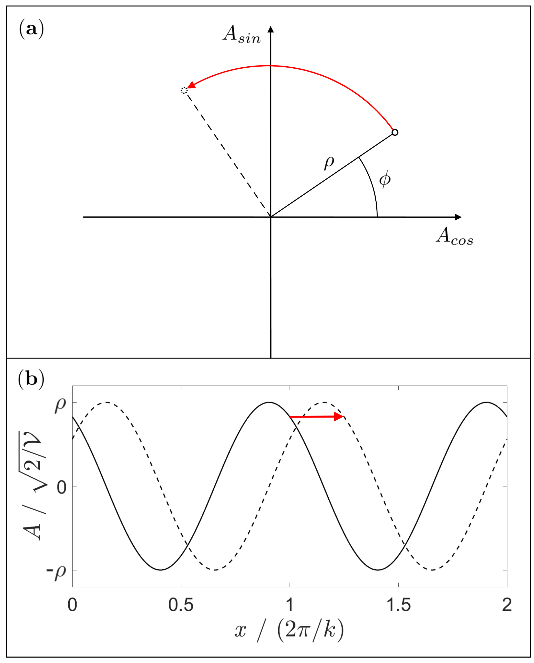 Figure 1
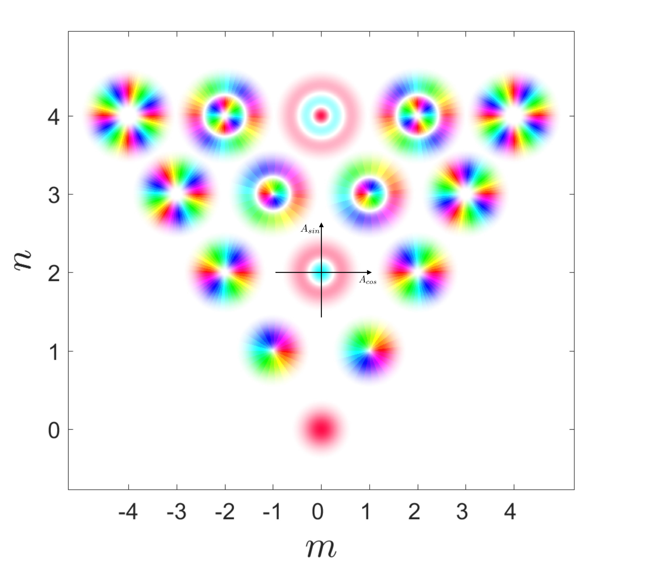 Figure 2
Peer Reviews
No public reviews on file for this paper yet. If you reviewed it on a platform where reviews are public (OpenReview, ICLR, NeurIPS, ICML), you can paste yours below so the community can read it here.
Videos
No videos yet. Explain this paper in a talk, walkthrough, or lecture? Add one.
Taxonomy
TopicsQuantum Information and Cryptography · Quantum Mechanics and Applications · Spectroscopy and Quantum Chemical Studies
Correction to the quantum phase operator for photons
Mads J. Damgaard
Niels Bohr Institute, University of Copenhagen, 2100 Copenhagen, Denmark
(March 1, 2024)
Abstract
The vector potential operator, , is transformed and rewritten in terms of cosine and sine functions in order to get a clear picture of how the photon states relate to the field. The phase operator, defined by , is derived from this picture. The result has a close resemblance with the known Susskind-Glogower (SG) operator, which is given by . It will be shown that should be replaced by instead to yield , which makes the operator unitary. will also be analyzed when restricted to the space of only forward moving photons with wave vector . The resulting phase operator, , will turn out to resemble the SG operator as well, but with a small correction: Whereas can be equivalently written as , the operator, , is instead given by , where . The sequence, , converges to from below for going to infinity.
Introduction
Electromagnetic waves are classically described by a wave vector, an amplitude and a phase. In quantum mechanics the concept of the wave vector remains the same, but the amplitude and the phase should now be represented by operators. Whereas there are general agreement about the amplitude operator, there has so far, according to Gerry and Knight [1], not been found a phase operator, that satisfies all the expected requirements. One of the quite successful proposals according to Gerry and Knight [1] is the Susskind-Glogower (SG) operator, which is given by
[TABLE]
or alternatively by
[TABLE]
Here, and are the creation and annihilation operators for photons with an implicit wave vector, , and is the state with of these photons. The SG operator is not supposed to represent the phase, , but the phase factor, . This means the SG operator is supposed to be unitary, but since
[TABLE]
this is not the case.
When I wrote my bachelor thesis [2], in which I looked at QED, my approach to the subject led me to quantize the electromagnetic field in terms of the cosine and sine Fourier components. This turned out to give a very neat picture of the quantum field with a quite easy interpretation of the photons, and where a unitary phase operator was easily derived.
In this paper I will summarize the resulting phase operator of my bachelor thesis [2], but instead of starting by considering the electromagnetic field and how to quantize it, I will obtain the same operator simply by deriving it from the well known operator, , representing the electromagnetic vector potential.
Resolving in terms of cosine and sine functions
To derive the phase operator in this paper, we will start by considering the operator representing the electromagnetic vector potential111We could just as well have chosen to look at the operator for the electric field, , instead since all of the following arguments apply for as well., , expressed in terms of creation and annihilation operators, where is a point in space. According to various textbooks, for example Gerry and Knight [1], we have
[TABLE]
where is the photon wave vector, labels the two polarizations, and are two unit vectors orthogonal to and to each other, , and is equal to the number of discrete values runs through. The operators and are the creation and annihilation operators, which respectively creates or annihilates a particle with wave vector and polarization . We choose to look at the discretized case where only take discrete values for simplicity. We will also need the commutation relations of the creation and annihilation operators, which are
[TABLE]
and we will need the Hamiltonian of the free photons, which is given by
[TABLE]
The idea is now rewrite in terms of cosine and sine functions. This can be done by introducing the operators and defined by
[TABLE]
These operators should only be defined for half of the -space, such that . Let therefore in both and , where . The inverted relations are
[TABLE]
Let us simplify the notation significantly in the following by suppressing some of the labels, except when we need to explicitly sum over them, and rewrite the operators as
[TABLE]
The above transformation of the creation and annihilation operators allows us to rewrite the contribution to coming from and . Let us call this contribution , such that
[TABLE]
where we have used the freedom in choosing the polarization vectors to set
[TABLE]
Using eq. (9) and (10), and suppressing the labels according to prescription (11), we can thus rewrite as
[TABLE]
The next step is to identify the operators and as the “position”222The quotation marks are used to remind the reader that the operator is not connected to the positions of the photons. It is instead connected with the amplitudes of the Fourier components of the field. operators in a two-dimensional harmonic oscillator system. To justify this, we need, firstly, to convince ourselves that , , and has the commutation relations of the ladder operators, i.e. that
[TABLE]
It is easy to see that these relations indeed follow from the original commutation relations of eq. (5). Secondly, we need to show that the contribution to coming from and , given by
[TABLE]
can be written equivalently as
[TABLE]
To show this, we only need to use the following, very useful relations for the number operators, obtained from eq. (9) and (10):
[TABLE]
and substitute them in eq. (16). This shows that , , and are indeed ladder operators in a two-dimensional harmonic oscillator system. Using the standard knowledge of harmonic oscillators, we can therefore rewrite in the more basic way in terms of Hermitian operators, , , and , as
[TABLE]
where
[TABLE]
This can easily be checked using the commutation relations of eq. (15). We can thus identify the two “position” operators in eq. (14) and finally rewrite as
[TABLE]
This concludes the transformation of and . Since the coefficients of and vanish in eq. (22), the resulting quantum system is very easy to interpret, as the relation between the photon states and the physical field is simple. To see this, let be the contribution to coming from the two Fourier coefficients, and let and be the observables associated with and . If we then consider a wave function, , defined on the -plane, we see from eq. (22) that each point, , in the plane corresponds to a physical configuration of the field. The absolute square of the amplitude, , thus represents the probability density of finding the amplitudes of the two Fourier components to be . Equation (20) furthermore tells us that the dynamics of are still simply those of a two-dimensional harmonic oscillator.
In the untransformed system where “position” and “momentum” operators are defined similarly to eq. (21) but in terms of and instead, the coefficients of the “momentum” operators do not vanish in the expression for . This is what makes the physical interpretation in this original system less immediate.
Let us consider the states created by and . These can be written as
[TABLE]
where and are non-negative integers denoting the numbers of photons with wave vector and respectively. When viewed in the -plane, these states can be identified333For a more thorough treatment of these angular momentum states of the two-dimensional harmonic oscillator, see Cohen-Tannoudji et al. [3]. as the simultaneous eigenstates of and the generator of rotations in the plane, , which is given by
[TABLE]
This fact can be seen by using relations (18) and (19) to rewrite in terms of number operators as
[TABLE]
It follows that
[TABLE]
which shows that is an eigenstate of .
The observable associated with is normally referred to as the “angular momentum” of the wave function. We will stick with this name in this paper, but this angular momentum of the wave function must not be confused with the actual, physical angular momentum of the photons. Remember that we are only looking at photons with a single, linear polarization, , which have no angular momentum by themselves. In fact, we see from eg. (26) that is instead proportional to the combined momentum of the photon states with proportionality constant , such that
[TABLE]
Here, is the momentum operator on the subspace of the states, such that the full photon momentum operator of the total -space, , is given by
[TABLE]
The relationship between and is in accordance with the fact that a rotation of the wave function in the -plane by an angle, , corresponds to a translation of the field by a distance of , as illustrated in fig. 2. Since is the generator of translations of , this is equivalent of stating that
[TABLE]
which is indeed true according to eq. (27).
The wave functions of the states, call them , can be calculated from eq. (23), using the relations for and given in eq. (9) and (10). Cohen-Tannoudji et al. [3] give the following results for the first six wave functions, , written in polar coordinates:
[TABLE]
Here, is the overall occupation number, and is the eigenvalue of , i.e. the overall momentum divided by . Whether is given in polar or Cartesian coordinates in the following will be clear from the context.
Figure (2) shows the first 15 photon wave functions, each plotted individually in the -plane and ordered next to each other in an -coordinate system.
As a final point in this section, let us define the complex amplitude operator, , by
[TABLE]
By using eq. (21) as well as eq. (9) and (10), we can rewrite in terms of and as
[TABLE]
If we label this by and , we see from eq. (4) that can thus be written as
[TABLE]
or, since ,
[TABLE]
Note that in terms of these equations, as well as eq. (22), is exactly like in the classical picture, just with hats put on the coefficients to mark them as operators.
The phase operator
Having transformed in terms of cosine and sine functions, it is now easy to identify the phase operator, . If we choose to represent the complex observable , such that
[TABLE]
then for all we simply have
[TABLE]
The fact that the denominator vanishes in is not a problem since one can always remove any finite number of points from the domain of the wave functions without changing the Hilbert space.444See for example Durhuus and Solovej [4], if not other literature on Hilbert spaces of square-integrable functions. The reason for this is connected with the fact that any vector in a Hilbert space must be uniquely determined by its inner products with all vectors in a complete basis. Since removing any point from the domain does not change any inner products on the space, the Hilbert space therefore remains unchanged. We can thus omit from the -plane. Note that removing a point from the domain does not change the differentiability of the wave functions either.
Having omitted from the -plane, we see that is now a strictly positive multiplicator on the plane. It is therefore evident that is positive definite, and it follows that we can take both the square root and the inverse of the operator. This means that can now be written in terms of and as
[TABLE]
It is remarkable how similar this expression looks to the SG operator of eq. (1). The only difference is that here, is replaced with instead. Whereas in eq. (1) had the effect of annihilating a photon, the effect of the replacement, , is now a superposition of the effects of annihilating a photon moving in one direction (the forward direction) and creating a photon moving in the opposite direction. Since the equation was derived from eq. (36), we see that this adjustment to the SG operator has the desired effect of making it unitary.
Since commutes with , it can be seen from eq. (37) that can only lower the eigenvalue of by for any of its eigenvectors. This fact can also be seen by considering the -dependency of the wave function for any eigenvector of , which is contained in the factor . Since the operator will send this into , the eigenvalue of will indeed be lowered by exactly . This means that will be orthogonal to any eigenvector, , for which . We can use this information to write as
[TABLE]
Note that every matrix element, , can be calculated once the wave functions of the two relevant states have been obtained, which can be done via eq. (23).
We can now ask ourselves the interesting question of what this new phase operator will become when it is restricted to a space containing only photons moving in the forward direction and no backward moving photons. This is the space on which previous phase operators such as the SG operator have been defined. This simplified operator, call it , can be of interest when considering a beam of photons rather than a cavity mode. We will define by
[TABLE]
such that
[TABLE]
for all . If we are interested in the expectation value of on this particular subspace, we can therefore just as well use instead of .
Let us analyze this operator, . We can start by noting that it is not unitary. This can be shown by calculating one of the non-zero matrix elements of that are set to zero in . We can for instance calculate the matrix element . Using eq. (30), we get
[TABLE]
Now, since
[TABLE]
we see that
[TABLE]
We can therefore conclude that is indeed not unitary. This fact might help us understand why no one has succeeded in finding an appropriate unitary phase operator when looking at photons with only a particular wave vector , and not at the same time including the photons with wave vector . The phase operator is simply not supposed to be unitary when restricted to this space.
Let us proceed to express in terms of its matrix elements. It turns out that there is a very neat formula for these. To get them, we will use the fact that, according to Cohen-Tannoudji et al. [3], the general wave function for is given in polar coordinates by
[TABLE]
The matrix element is therefore given by
[TABLE]
where we have changed the integration variable to to get the third equality and then identified the resulting integral as the gamma function. If we write more compactly as , we see that eq. (39) now becomes
[TABLE]
The sequence
[TABLE]
is convergent, and it converges to . A way to see this is to use the duplication formula:
[TABLE]
Stirling’s approximation tells us that
[TABLE]
for tending toward infinity, and therefore we have
[TABLE]
To show that for all , one can quite easily calculate to show that for all . The strictly increasing sequence will therefore never reach 1.
The similarity between our and the SG operator, which is also defined on the space of states with only forward moving photons, is now even more striking. If we rename all as , , for compactness, we can write as
[TABLE]
Meanwhile, the SG operator, as we recall, is given by
[TABLE]
This shows that the SG operator is a very good approximation to , especially for large occupation numbers. We just need to remember that represents in this paper, and not like it does, for instance, in Gerry and Knight [1].
A natural question we can ask ourselves moving on is what the uncertainty is on a measurement of the phase factor of a beam of photons. Since is not hermitian, we cannot use the commutator to get a lower limit on e.g. . We can, however, still calculate the variance of for any state in the full Hilbert space. It is given by
[TABLE]
When we are interested in a state with only forward moving photons, , we can thus use eq. (40) and (51) to obtain
[TABLE]
To check that the RHS of this formula is greater than [math], define two new vectors: and . Note that , and therefore, due to the Cauchy-Schwarz inequality,
[TABLE]
Following up on this, we can use eq. (54) to try searching for a state, , that minimizes . If we define a state, , by
[TABLE]
we have, for large enough ,
[TABLE]
This result goes to [math] as goes to infinity, and we can therefore get an arbitrarily small by choosing large enough. This shows that we can still get an arbitrarily precise phase for a photon beam even without any backward moving photons. The time evolution of this is given by
[TABLE]
and therefore the time evolution of the expectation value of is
[TABLE]
for large enough . The result tends toward as tends to infinity, which is as expected for a coherent photon beam.
As a final remark in this paper, I will point out that it might be beneficial to look at operators or instead of when analyzing the time evolution or the uncertainty of the field, especially when it contains both backward and forward moving photons. This should make the calculation easier since these operators contain only positive, integer powers of the ladder operators. If, for instance, one wants to find the behavior of the field of a coherent cavity mode, one might therefore choose to look at the expectation value of .
Conclusion
We have derived the photon phase operator starting from just the well known vector potential operator, , and the well known Hamiltonian for photons. As it turned out, only a simple transformation was needed to make exactly analogous to the expression for the classical field. From there the phase operator was derived easily. The result was similar to the well known SG operator, but defined on a larger space with photons having wave vectors equal to both and . It seems that the reason why no one has found a satisfactory, unitary phase operator so far might be because no one has tried including the backward moving photons in the domain of the operator and tried to combine both and in the definition. When restricted to the space of photons with wave vectors only equal to , setting all other matrix elements to zero, the phase operator turned out to be numerically very close to the SG operator as well. The correction is a factor of on the th matrix element for all , and this correction becomes less significant with increasing photon number.
The reference list from the paper itself. Each links out to its DOI / PubMed record.
- 1[1] C. C. Gerry and P. L. Knight, Introductory Quantum Optics (Cambridge University Press, Cambridge, 2005).
- 2[2] M. J. Damgaard, B.Sc. thesis, Niels Bohr Institute, 2017.
- 3[3] C. Cohen-Tannoudji, B. Diu, and F. Laloë, Quantum Mechanics (John Wiley & Sons, New York, 1977), Vol. 1, Chap. VI, Compliment D VI .
- 4[4] B. Durhuus and J. P. Solovej, Mathematical Physics , Lecture notes, Department of Mathematical Sciences, University of Copenhagen, 2014.