Taxonomy Induction using Hypernym Subsequences
Amit Gupta, R\'emi Lebret, Hamza Harkous, Karl Aberer

TL;DR
This paper introduces a semi-supervised method for domain taxonomy induction that leverages hypernym subsequences within a probabilistic framework, outperforming existing methods and demonstrating robustness to noisy input vocabularies across multiple languages.
Contribution
It presents a novel hypernym subsequence extraction approach and formulates taxonomy induction as a minimum-cost flow problem, improving robustness and accuracy.
Findings
Outperforms state-of-the-art methods across four languages.
Demonstrates robustness to noisy input vocabularies.
Effective in extracting hypernym subsequences for taxonomy induction.
Abstract
We propose a novel, semi-supervised approach towards domain taxonomy induction from an input vocabulary of seed terms. Unlike all previous approaches, which typically extract direct hypernym edges for terms, our approach utilizes a novel probabilistic framework to extract hypernym subsequences. Taxonomy induction from extracted subsequences is cast as an instance of the minimumcost flow problem on a carefully designed directed graph. Through experiments, we demonstrate that our approach outperforms stateof- the-art taxonomy induction approaches across four languages. Importantly, we also show that our approach is robust to the presence of noise in the input vocabulary. To the best of our knowledge, no previous approaches have been empirically proven to manifest noise-robustness in the input vocabulary.
Click any figure to enlarge with its caption.
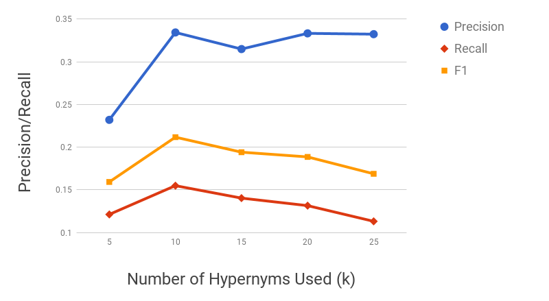 Figure 1
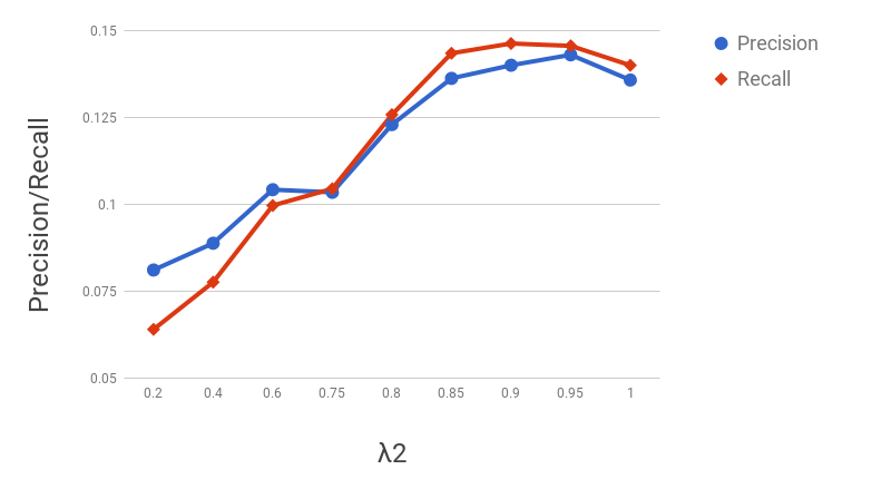 Figure 2
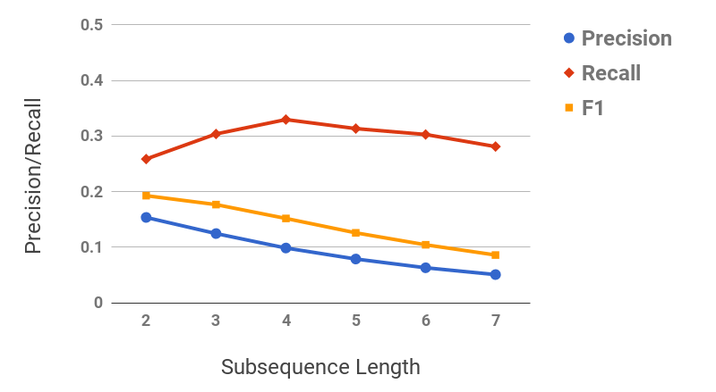 Figure 3
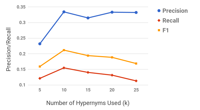 Figure 4
 Figure 5
 Figure 6
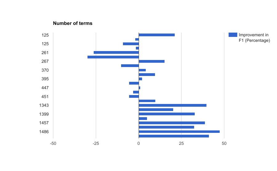 Figure 7
 Figure 8
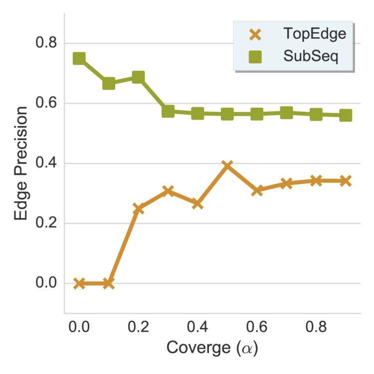 Figure 9
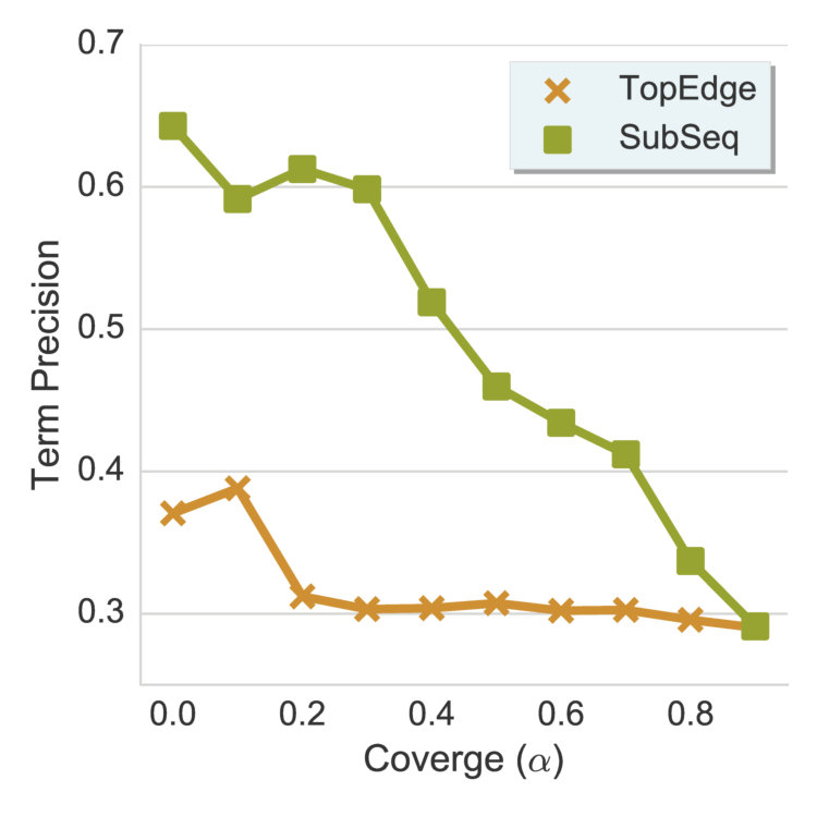 Figure 10
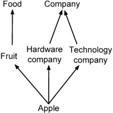 Figure 11
 Figure 12
 Figure 13
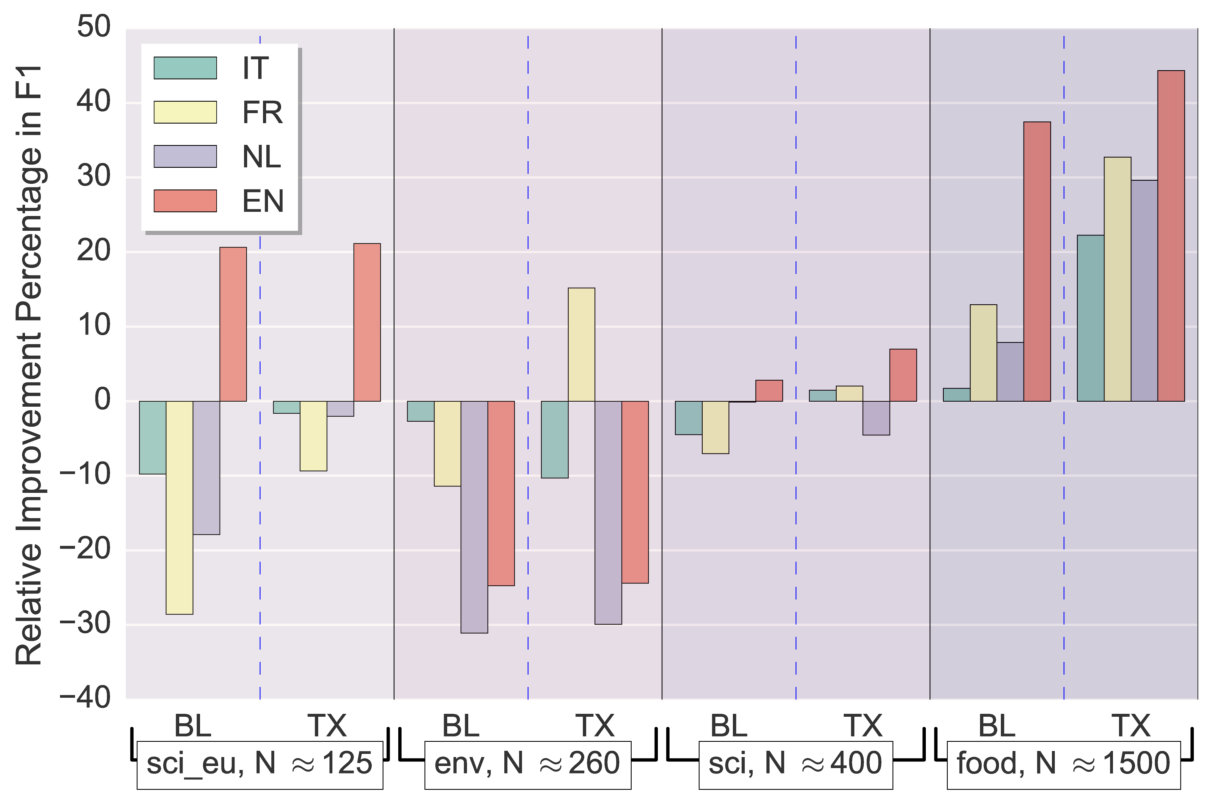 Figure 14
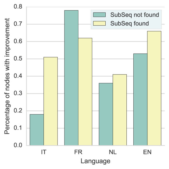 Figure 15
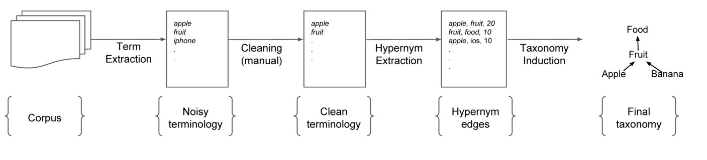 Figure 16
 Figure 17
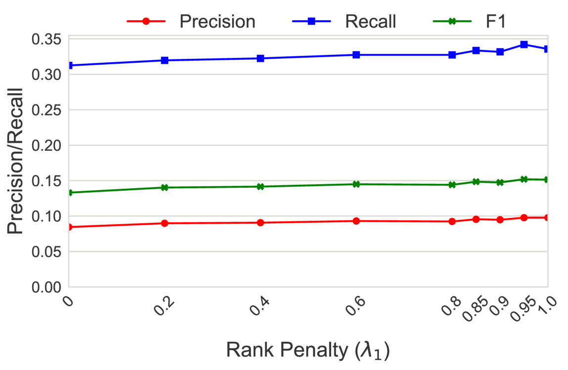 Figure 18
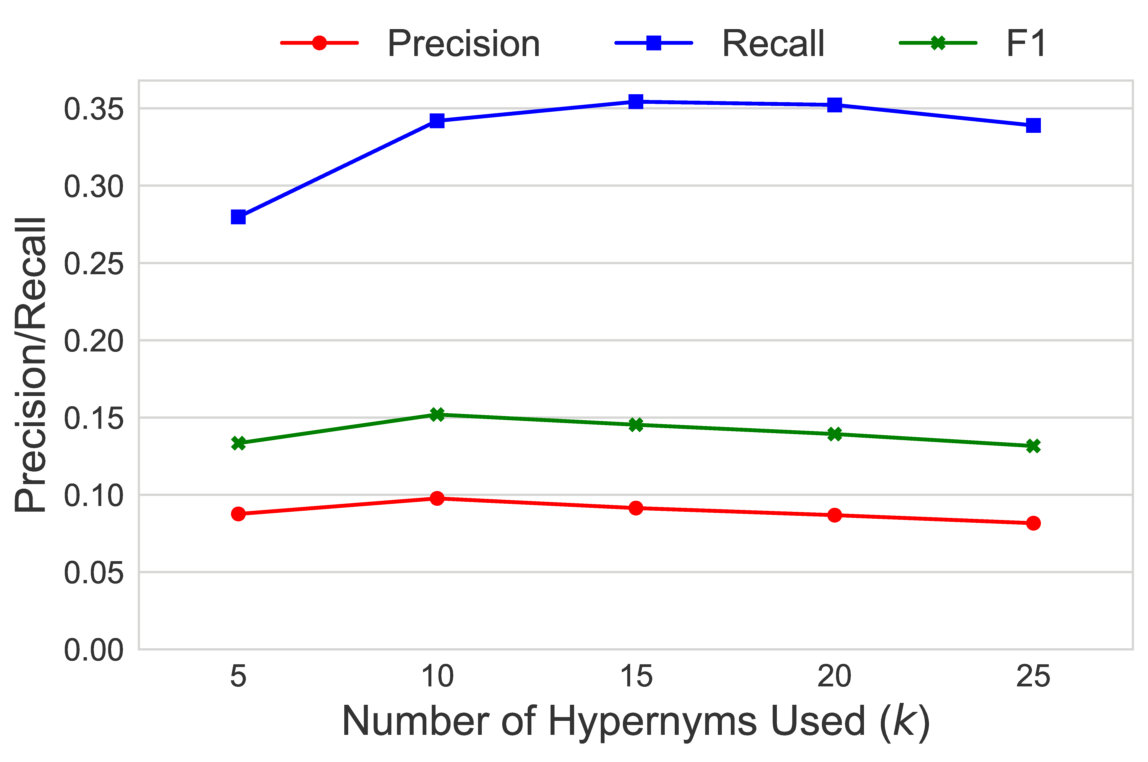 Figure 19
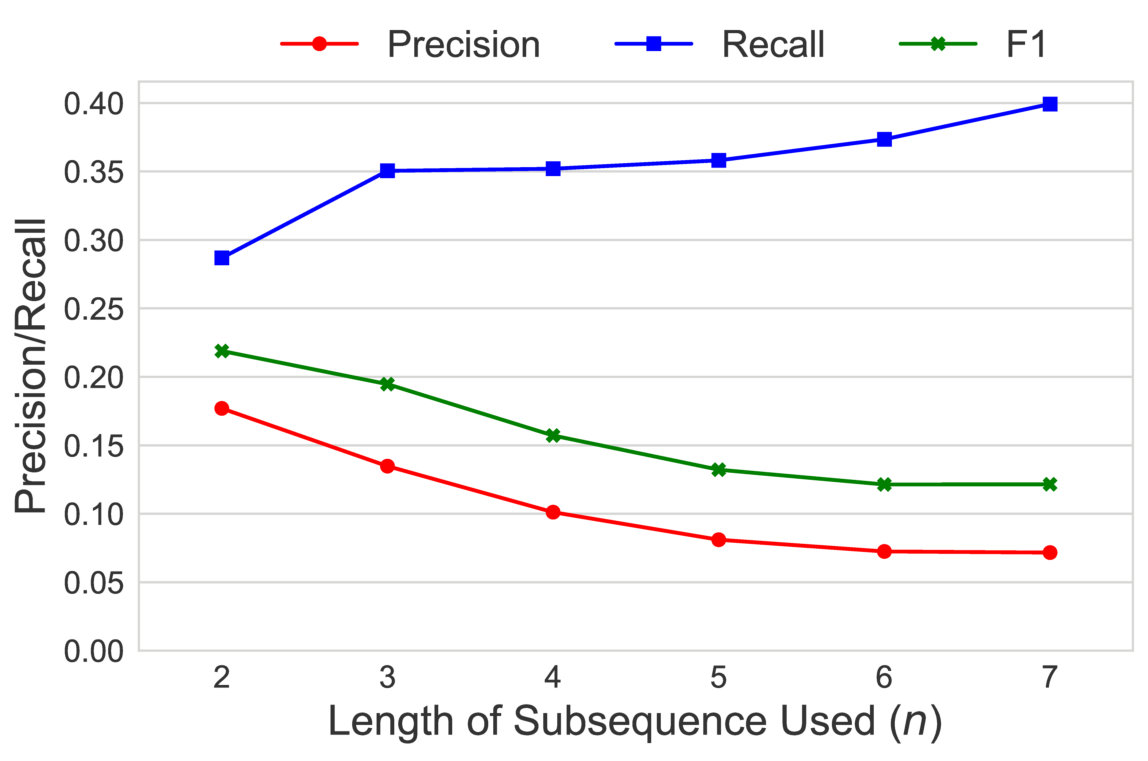 Figure 20
 Figure 21
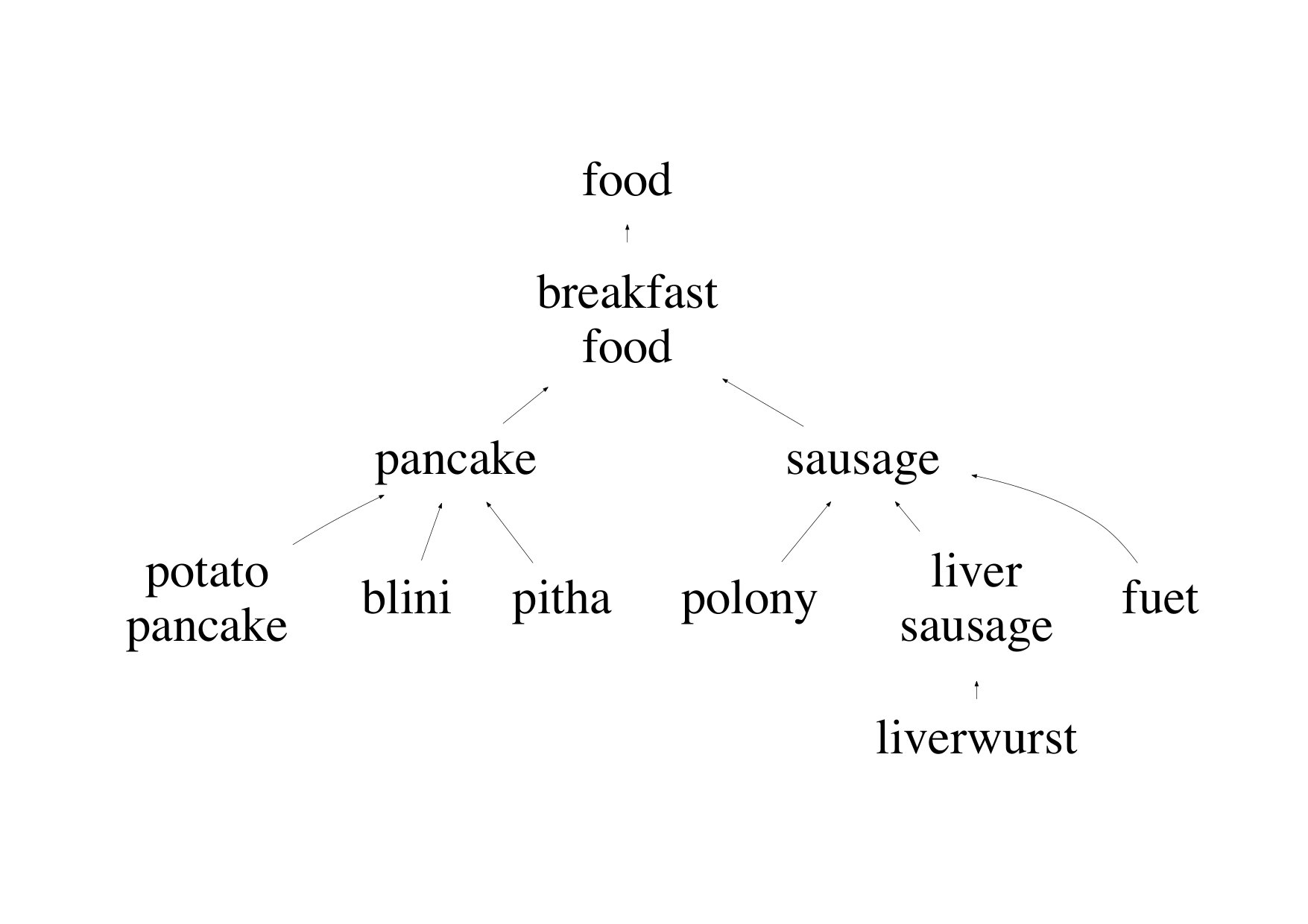 Figure 22
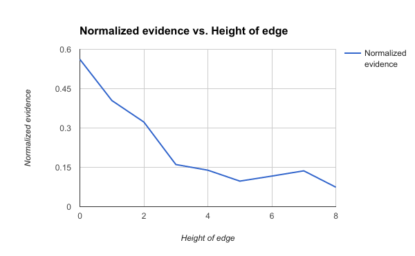 Figure 24
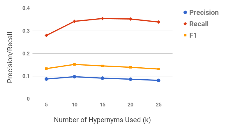 Figure 25
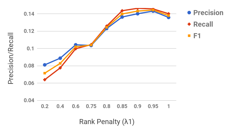 Figure 26
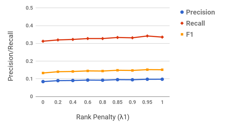 Figure 27
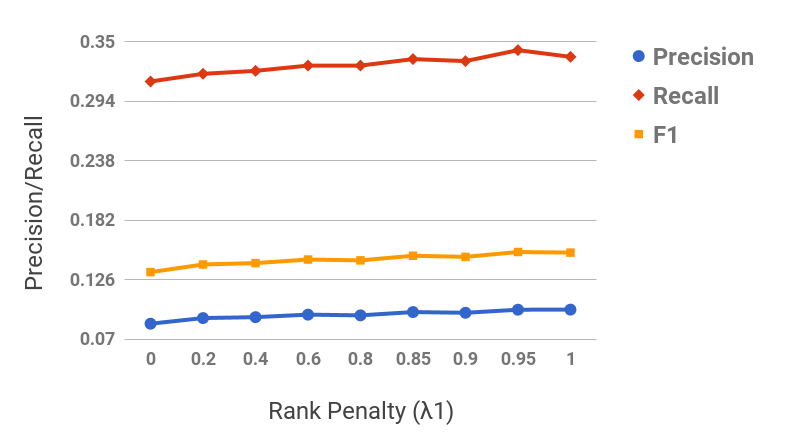 Figure 28
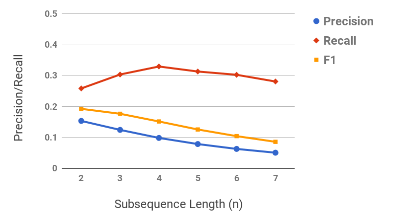 Figure 29
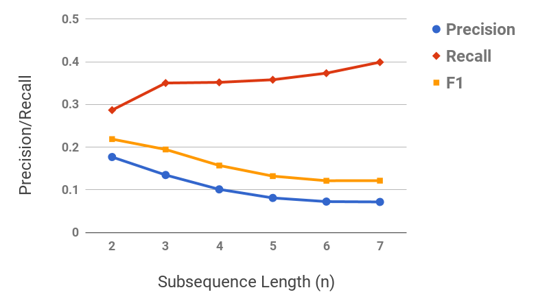 Figure 30
 Figure 36
 Figure 37
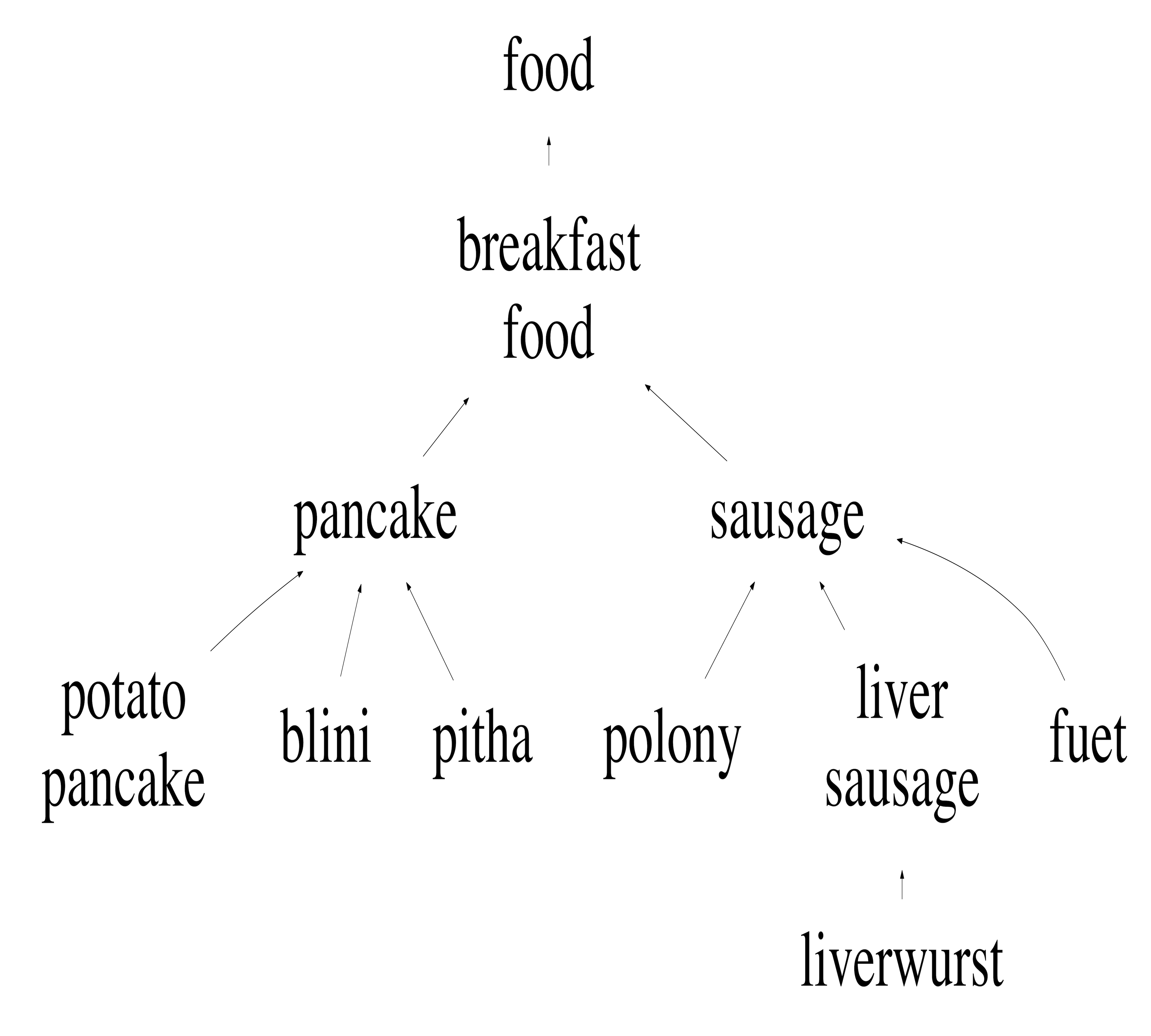 Figure 38
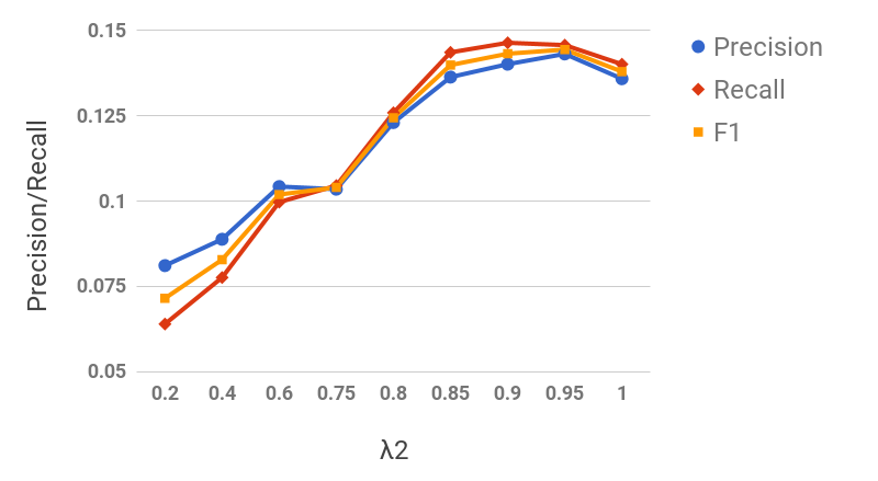 Figure 39
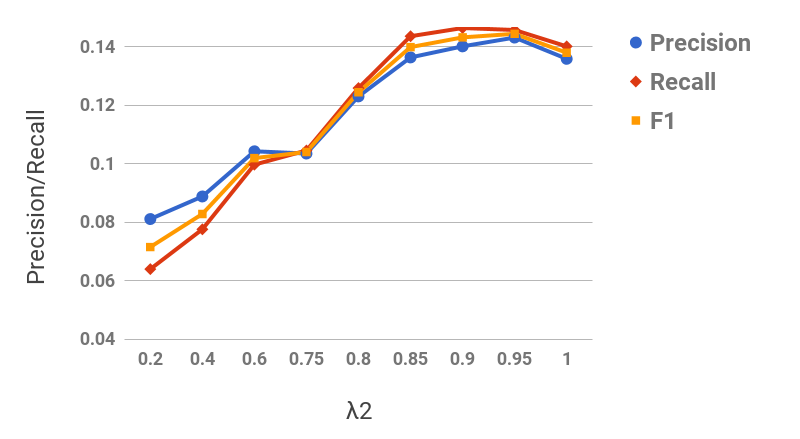 Figure 40
| Candidate hypernym | Frequency |
|---|---|
| company | 5536 |
| fruit | 3898 |
| apple | 2119 |
| vegetable | 928 |
| orange | 797 |
| tech company | 619 |
| brand | 463 |
| hardware company | 460 |
| technology company | 427 |
| food | 370 |
| Initial subsequences |
|---|
| mortadellasausagemeatfood |
| laksasoupdishfood |
| Expanded subsequences |
| mortadellalarge Italian sausagesausageprocess meatmeatfood |
| laksaspicy noodle soupnoodle soupsoupdishfood |
| TAXI | SubSeq | |||||
|---|---|---|---|---|---|---|
| P | R | F1 | P | R | F1 | |
| EN | 33.2 | 31.7 | 32.2 | 44.9 | 31.9 | 37.2 |
| NL | 48.0 | 19.7 | 27.6 | 42.3 | 20.7 | 27.9 |
| FR | 33.4 | 24.1 | 27.7 | 41.0 | 24.4 | 30.5 |
| IT | 53.7 | 20.7 | 29.1 | 49.0 | 21.8 | 29.9 |
Peer Reviews
No public reviews on file for this paper yet. If you reviewed it on a platform where reviews are public (OpenReview, ICLR, NeurIPS, ICML), you can paste yours below so the community can read it here.
Videos
No videos yet. Explain this paper in a talk, walkthrough, or lecture? Add one.
\xpatchcmd
Taxonomy Induction Using Hypernym Subsequences
Amit Gupta
EPFL, Lausanne, Switzerland
,
Rémi Lebret
EPFL, Lausanne, Switzerland
,
Hamza Harkous
EPFL, Lausanne, Switzerland
and
Karl Aberer
EPFL, Lausanne, Switzerland
(2017)
Abstract.
We propose a novel, semi-supervised approach towards domain taxonomy induction from an input vocabulary of seed terms. Unlike all previous approaches, which typically extract direct hypernym edges for terms, our approach utilizes a novel probabilistic framework to extract hypernym subsequences. Taxonomy induction from extracted subsequences is cast as an instance of the minimum-cost flow problem on a carefully designed directed graph. Through experiments, we demonstrate that our approach outperforms state-of-the-art taxonomy induction approaches across four languages. Importantly, we also show that our approach is robust to the presence of noise in the input vocabulary. To the best of our knowledge, this robustness has not been empirically proven in any previous approach.
Knowledge acquisition; taxonomy induction; term taxonomies; algorithms; flow networks; minimum-cost flow optimization;
††copyright: rightsretained††journalyear: 2017††copyright: acmlicensed††conference: CIKM’17 ; November 6–10, 2017; Singapore, Singapore††price: 15.00††doi: 10.1145/3132847.3133041††isbn: 978-1-4503-4918-5/17/11††ccs: Computing methodologies Artificial intelligence††ccs: Computing methodologies Information extraction††ccs: Computing methodologies Ontology engineering††ccs: Computing methodologies Semantic networks
1. Introduction
Motivation.
Lexical semantic knowledge in the form of term taxonomies has been beneficial in a variety of NLP tasks, including inference, textual entailment, question answering and information extraction (Biemann, 2005). This widespread utility of taxonomies has led to multiple large-scale manual efforts towards taxonomy induction, such as WordNet (Miller, 1994) and Cyc (Lenat, 1995). However, such manually constructed taxonomies suffer from low coverage (Hovy et al., 2009) and are unavailable for specific domains or languages. Therefore, in recent years, there has been substantial interest in extending existing taxonomies automatically or building new ones (Snow et al., 2006; Yang and Callan, 2009; Kozareva and Hovy, 2010; Velardi et al., 2013; Bordea et al., 2015; Bordea et al., 2016).
Approaches towards automated taxonomy induction consist of two main stages:
- (1)
extraction of hypernymy relations (i.e., “is-a” relations between a term and its hypernym such as applefruit) 2. (2)
structured organization of terms into a taxonomy, i.e., a coherent tree-like hierarchy.
Extraction of hypernymy relations has been relatively well-studied in previous works. Its approaches can be classified into two main categories: Distributional and Pattern-based approaches.
Distributional approaches use clustering to extract hypernymy relations from structured or unstructured text. Such approaches draw primarily on the distributional hypothesis (Harris, 1954), which states that semantically similar terms appear in similar contexts. The main advantage of distributional approaches is that they can discover relations not directly expressed in the text.
In contrast, Pattern-based approaches utilize pre-defined rules or lexico-syntactic patterns to extract terms and hypernymy relations from text (Hearst, 1992; Oakes, 2005). Patterns are either chosen manually (Hearst, 1992; Kozareva et al., 2008) or learnt automatically via bootstrapping (Snow et al., 2004). Pattern-based approaches usually result in higher accuracies. However, unlike the distributional approaches, which are fully unsupervised, they require a set of seed surface patterns to initiate the extraction process.
Early work on the second stage of taxonomy induction, namely the structured organization of terms into a taxonomy, focused on extending existing partial taxonomies such as WordNet by inserting missing terms at appropriate positions (Widdows, 2003; Snow et al., 2006; Yang and Callan, 2009). Another line of work focused on taxonomy induction from Wikipedia by exploiting the semi-structured nature of the Wikipedia category network (Suchanek et al., 2007; Ponzetto and Strube, 2008, 2011; Nastase et al., 2010; Flati et al., 2016; Gupta et al., 2016).
Subsequent approaches to taxonomy induction focused on building lexical taxonomies entirely from scratch, i.e., from a domain corpus or the Web (Kozareva and Hovy, 2010; Navigli et al., 2011; Velardi et al., 2013; Bansal et al., 2014; Alfarone and Davis, 2015; Panchenko et al., 2016).
Automated taxonomy induction from scratch is preferred because it can be used over arbitrary domains, including highly specific or technical domains, such as Finance or Artificial Intelligence (Navigli et al., 2011). Such domains are usually under-represented in existing taxonomic resources. For example, WordNet is limited to the most frequent and the most important nouns, adjectives, verbs, and adverbs (Gurevych and Wolf, 2010; Nakashole et al., 2012). Similarly, Wikipedia is limited to popular entities (Kliegr et al., 2014), and its utility is further diminished by slowed growth (Suh et al., 2009).
Past approaches to taxonomy induction from scratch either assume the availability of a clean input vocabulary (Panchenko et al., 2016) or employ a time-consuming manual cleaning step over a noisy input vocabulary (Velardi et al., 2013). For example, Figure 1 shows the pipeline of a typical taxonomy induction approach from a domain corpus (Velardi et al., 2013). An initial noisy vocabulary is automatically extracted from the domain corpus using a term extraction tool, such as TermExtractor (Sclano and Velardi, 2007), and is further cleaned manually to produce the final vocabulary. This requirement severely limits the applicability of such approaches in an automated setting because clean vocabularies are usually unavailable for specific domains.
To handle these limitations, we designed our approach to induce a taxonomy directly from a noisy input vocabulary. Consequently, it is the first work to fully automate the taxonomy induction process for arbitrary domains.
Contributions.
In this paper, we present a novel, semi-supervised approach for building lexical taxonomies given an input vocabulary of (potentially noisy) seed terms. We leverage the existing work on hypernymy relations extraction and focus on the second stage, i.e. the organization of terms into a taxonomy. Our main contributions are as follows:
- •
We propose a novel probabilistic framework for extracting longer hypernym subsequences from hypernymy relations, as well as a novel minimum-cost flow based optimization framework for inducing a tree-like taxonomy from a noisy hypernym graph.
- •
We empirically show that our approach outperforms state-of-the-art taxonomy induction approaches across four different languages, while achieving 32% relative improvement in F1-measure over the Food domain.
- •
We demonstrate that our subsequence-based model is robust to the presence of noisy terms in the input vocabulary, and achieves a 65% relative improvement in precision over an edge-based model while maintaining similar coverage. To the best of our knowledge, this is the first approach towards taxonomy induction from a noisy input vocabulary.
The rest of the paper is organized as follows. In Section 2, we describe our taxonomy induction approach. In Section 3, we discuss our experiments and performance results. In Section 4, we discuss related work. We conclude in Section 5.
2. Taxonomy Induction
Given a potentially-noisy vocabulary111In this work, we use terminology and vocabulary interchangeably. of seed terms as an input, we define our goal as inducing a taxonomy consisting of these seed terms (and possibly other terms). This taxonomy is a directed acyclic graph with terms as the nodes and the edges indicating a hypernymy relationship between the terms. For our task, we assume the availability of a database of candidate hypernymy relations. Multiple such resources have been compiled and made available publicly over the years. A prominent example of such a resource is WebIsA (Seitner et al., 2016), a collection of more than 400 million hypernymy relations for English, extracted from the CommonCrawl web corpus using lexico-syntactic patterns. However, such resources come with a considerable number of noisy candidate hypernyms, typically containing a mixture of relations such as hyponymy, meronymy, synonymy and co-hyponymy. For example, WebIsA has more than 12,000 hypernyms for the term apple, including noisy hypernyms such as orange, everyone and smartphone. A sample set of candidate hypernyms and their occurrence frequencies for the term apple taken from WebIsA is shown in Table 1.
Our approach to taxonomy induction consists of three main steps:
- (1)
extracting hypernym subsequences for the given seed terms (Section 2.1), 2. (2)
aggregating the extracted subsequences into an initial hypernym graph (Section 2.2), 3. (3)
pruning the hypernym graph using a minimum-cost flow approach to induce the final taxonomy (Section 2.3).
2.1. Hypernym Subsequences Extraction
Unsupervised or semi-supervised approaches to taxonomy induction typically aim to extract single hypernym edges among terms from noisy candidate hypernyms (Kozareva and Hovy, 2010; Panchenko et al., 2016). In contrast, our approach consists of extracting hypernym subsequences (where a subsequence is a series of one or more individual hypernym edges).
To motivate this, we first note that Table 1 includes hypernyms of apple at different levels of generality, such as fruit and food. In fact, we observe this pattern in the candidate hypernyms of most terms. This suggests that we can leverage such information to not only extract the direct hypernyms of apple, but to also extract longer hypernym subsequences, such as applefruitfood.
This becomes even more important given the result by Velardi et al. (2013), who demonstrated that hypernym extraction becomes increasingly erroneous as the generality of terms increases, mainly due to the increase in term ambiguity. To further support this hypothesis, we perform an experiment where we first randomly sample 100 paths from Wordnet. For each edge a$$\rightarrow$$b in a sampled path, we plot the normalized frequency222Normalization is performed by dividing frequency counts by the maximum. of “ as a candidate hypernym for ” against the height of the edge, where frequencies are computed using lexico-syntactic patterns (cf. Table 1). We also plot the average rank of among candidate hypernyms of , where candidate hypernyms are ranked by their normalized frequencies in a decreasing order. Results of this experiment are shown in Figure 2. Since edges in WordNet are assumed to be ground truth, it is desired that they have a higher normalized frequency and lower ranks. This small-scale experiment demonstrates that as the height of the edge increases, the normalized frequencies decrease whereas the average ranks increase. Therefore, the accuracy of patterns-based hypernymy detection decreases for more general terms that appear higher in generalization paths. Hence, for such terms, it makes sense to not solely base the hypernym selection on a noisy set of candidate hypernyms. We can potentially improve the accuracy of selected hypernyms for general terms (such as fruit) by relying on extracted subsequences starting from more specific terms (such as apple). Those subsequences would be evidenced by the less-noisy candidate hypernyms of the specific terms.
In sum, extracting hypernym subsequences is both possible and potentially beneficial. The remainder of this section describes our model that realizes this intuition.
Model.
We now describe our model for extracting hypernym subsequences for a given term. We begin with a general formulation using directed acyclic graphs (referred to as DAG), and we make simplifying assumptions to derive a model for hypernym subsequences. We use the following notations:
- •
: a given seed term, e.g., apple;
- •
: lexical head of any term , e.g., =soup for =chicken soup;
- •
: Hypernym Evidence, i.e., the set of all the candidate hypernymy relations, in the form of 3-tuples (hyponym, hypernym, frequency);
- •
: Hypernym Evidence for term , i.e., the set of top- candidate hypernyms for term , having the highest frequency counts (Table 1 shows a sample from for =apple);
- •
: mth ranked candidate hypernym from , where , and ranks are computed by sorting candidate hypernyms in decreasing order of frequency counts;
- •
: A similarity measure between terms and estimated using evidence ;
- •
: a DAG consisting of generalizations for a term (Figure 3 shows an example of a possible DAG for t$$=apple).
For a given term , we define the goal of this step of our taxonomy induction approach as finding a DAG , which maximizes the conditional probability of , given the evidence , for a fixed :
[TABLE]
Due to the combinatorial nature of the search space of , finding an exact solution to the above equation is intractable, even for a small . Therefore, we make the following simplifying assumptions, which facilitate an efficient search through the search space of :
- •
can be approximated as a set of independent hypernym subsequences with possibly repeated hypernyms. In other words, where is the subsequence and is a fixed constant. For example, the DAG shown in Figure 3 can be approximated as a set of three subsequences: (i) applefruitfood, (ii) applehardware companycompany, and (iii) appletechnology companycompany. This assumption intuitively derives from the fact that any DAG can be represented by a finite number of subsequences.
- •
, the joint events are independent. Intuitively, this assumption implies that each subsequence independently contributes to the evidence .
- •
, the direct hypernyms of in are unique. In other words, for a candidate hypernym of given term , there is at most one subsequence with the first edge t_{0}$$\rightarrow$$h_{c}. Intuitively, this assumption implies that a candidate hypernym uniquely sense-disambiguates the term , thus resulting in a only one possible generalization subsequence.
In conjunction, these assumptions imply that is composed of hypernym subsequences, where each subsequence independently attempts to generate . Given these assumptions, Equation 1 transforms into:
[TABLE]
Estimation.
We now describe the estimation of and for a hypernym subsequence . In order to motivate the estimation of the conditional probability , we start with an example. Consider a valid hypernym subsequence applefruitfoodsubstancematterentity for the term apple (whose candidate hypernyms are in Table 1). At first sight, it might seem desirable for a candidate hypernym from (e.g., fruit) to have a high similarity with as many terms in the subsequence as possible. However, since the similarity measure is based on the hypernym evidence , it is plausible that terms such as matter and entity have a low similarity with the candidate hypernym fruit, simply because they are at a higher level of generality. To avoid penalizing such valid subsequences, we let the conditional probability be proportional to the maximum similarity possible between the candidate hypernym and any term in the subsequence (e.g., for the candidate hypernym fruit, the similarity is 1 as fruit is in the subsequence). We aggregate those similarity values across the candidate hypernyms. More formally, assuming subsequence = t_{0}$$\rightarrow$$h_{i1}$$\rightarrow$$h_{i2}…, where is the length of , we compute the conditional probability as:
[TABLE]
where (a fixed parameter) serves as a rank-penalty to penalize candidate hypernyms with lower frequency counts.
We now proceed to compute , the other constituent of Equation 2. Towards that, we assume that is a collection of independent hypernym edges. Thus, becomes the product of the individual edges’ probabilities:
[TABLE]
where is the probability of an individual hypernym edge x_{1}$$\rightarrow$$x_{2} between terms and ; is a length penalty parameter.
Finally, we estimate as a log-linear model using a set of features f, weighted by the learned weight vector w:
[TABLE]
We also use this edge probability to compute the aforementioned similarity function (sim) as:
[TABLE]
Intuitively, promotes subsequences containing a larger number of candidate hypernyms from whereas promotes subsequences consisting of individual edges with a larger probability of hypernymy.
Subsequence Extraction.
After inserting Equations 3 and 4 into Equation 2 and taking logarithm, the objective function becomes:
[TABLE]
This objective function leads to the following search algorithm for the extraction of subsequences:
- (1)
For a given term , iterate over all candidate hypernyms in . 2. (2)
For each , perform a depth-limited beam search over the space of possible subsequences by recursively exploring the candidate hypernyms of (i.e., . 3. (3)
For each , choose the subsequence with the highest score (i.e., . 4. (4)
Choose the top- candidate hypernyms based on their corresponding subsequence scores.
While, in theory, we can iterate over all candidate hypernyms in , in practice, we employ an alternative two-stage execution that significantly improves the running time as well as produces more meaningful subsequences:
Search phase: Proceed as in the aforementioned steps. However, in the special case where a candidate hypernym is a compound term and its lexical head is also present in , skip in step (1) of the algorithm333Lexical heads of terms have consistently played a special role in taxonomy induction (Ponzetto and Strube, 2011; Gupta et al., 2016).. For example, for apple, candidate hypernyms tech company, software company and hardware company are skipped in step (1) due to the presence of company in (cf. Table 1).
Expansion phase: In this phase, we augment the subsequences extracted in the search phase to account for skipped compound terms. We focus on the case where the lexical head of the skipped compound terms occurs in a subsequence. In that case, we expand the incoming edge of the lexical head with zero or more of those compound terms. For example, in the subsequence applecompanyorganization, a potential expansion of the edge applecompany is: appleAmerican software companysoftware companycompany. However, special attention has to be taken while generating these potential expansions. For example, the expansion appleAmerican software companyBritish software companycompany is invalid due to the co-hyponymy edge American software companyBritish software company. In contrast, the expansion appleAmerican software companysoftware companycompany is a valid expansion. To avoid invalid expansions, we restrict the possible expansions to the case where the set of pre-modifiers of a compound term is a superset of its hypernym’s pre-modifiers (e.g., {American, software }{software}).
We generate all possible expansions for each edge and rank them by averaging a TF-IDF-style metric across the pre-modifiers of compound terms in each expansion. Our aim in the ranking is two-fold: i) promoting the pre-modifiers, which frequently appear in the evidence , and ii) penalizing the noisy pre-modifiers unrelated to that frequently occur in compound terms (e.g., several, other, etc.). Hence, we compute the TF score of a pre-modifier as its average frequency of occurrence in the candidate hypernyms . We compute IDF as the average frequency of occurrences of the pre-modifier in for a random term . Finally, we choose the top ranked expansion per edge.
To illustrate the result of the previous steps, we show in Table 2 an example of extracted subsequences along with their expanded versions for the food domain. Intuitively, the two-stage execution serves to distinguish between two fundamentally different forms of generalization:
- (1)
type-based generalization, which provides core types as generalizations (e.g., applecompanyorganization). 2. (2)
attribute-based generalization, which enriches type-based generalization edges. For example, appleamerican software companysoftware companycompany enriches the individual type-based edge applecompany.
In our experiments, models that distinguished between these two different forms of generalizations consistently performed better than models, which attempted to unify them.
Features.
We now describe the edge features that we employ for estimating the probability of a hypernymy relation between two terms (cf. Equation 5):
Normalized Frequency Diff (): Similar to (Panchenko et al., 2016), this feature is an asymmetric hypernymy score based on frequency counts. We compute by first normalizing the frequency counts obtained (i.e., the counts in ) for term as follows: , where is the frequency count of candidate hypernym in . Further, we subtract the score in the opposite direction to downrank synonyms and co-hyponyms: .
Generality Diff (): We introduce a novel feature for explicitly incorporating the term generality (or abstractness) in our model. To this end, we first define the generality of a term as the log of the number of distinct hyponyms present in all candidate hypernymy relations (); i.e., g(t)=\text{log}(1+\lvert x\mid x$$\rightarrow$$t\in E\rvert). We define the generality of an edge as the difference in generality between the hypernym and the hyponym: .
Intuitively, we aim to promote edges with the right level of generality and penalize edges, which are either too general (e.g., applething) or too specific (i.e., edges between synonyms or co-hyponyms, such as appleorange). To realize this intuition, we first sample a random set of terms and collect the edges with highest for these terms (hereafter referred to as top edges). We compare the distribution of generality (i.e., ) for the top edges vs. the distribution of generality for a set of randomly sampled edges. The assumption is that it is more likely to sample the generality of a correct edge (i.e., edge at right level of generality) from the distribution of top edges as compared to random edges. Hence, given and as the Gaussian distributions estimated from the samples of generality for top edges and random edges respectively, we define the feature as: g_{d}(x_{i},x_{j})=\text{Pr}_{D_{t}}\big{(}g_{e}(x_{i},x_{j})\big{)}-\text{Pr}_{D_{r}}\big{(}g_{e}(x_{i},x_{j})\big{)}.
Parameter Tuning.
We estimate the weights for features (w in equation 5), using a support vector machine trained on a manually annotated set of 500 edges. For beam search in the search phase, we use a beam of width 20, and limit the search to subsequences of maximum length 4. We set the rest of the parameters by running grid-search over a manually-defined range of parameters using a small validation set444Validation set is excluded from the test set.. The final values of parameters are as follows: k$$=$$10, b$$=$$4, \lambda_{1}$$=$$\lambda_{2}$$=$$0.95.
2.2. Aggregation of Subsequences
Up till now, we have described our methodology to generate hypernym subsequences starting from a given term. In this section, we aggregate the hypernym subsequences obtained for a set of seed terms, in order to construct an initial hypernym graph. For that, we undertake the following steps:
Domain Filtering.
Given a term , the usual case is that multiple hypernym subsequences corresponding to different senses of the term are extracted. For example, apple can be a company or a fruit, thus resulting in subsequences applefruitfood and applesoftware companycompany. However, many of these subsequences will not pertain to the domain of interest (as determined by the seed terms). To eliminate the irrelevant ones, we estimate a smoothed unigram model555We used a weighting function (i.e., step function with cut-off at 50% of the height of the subsequence) to favor terms at lower heights as they are usually more domain-specific. from all extracted subsequences, and we remove those with generation probabilities below a fixed threshold.
Hypernym Graph Construction.
We now aggregate the filtered subsequences into an initial hypernym graph. We construct this graph by grouping the edges with the same start and end nodes together from the filtered subsequences. The weight of each edge is computed as the sum of the scores of subsequences it belongs to (i.e., ( ). To increase the coverage for compound seed terms that do not yet have a hypernym, we simply add an hypernym edge to their lexical head with weight=$$\infty (i.e, a very large value) whenever the lexical head is already present in the hypernym graph. Finally, for each cycle in the hypernym graph, we remove the edge with the smallest weight, hence resulting in a DAG. This DAG contains many noisy terms and edges, which are pruned in the next step of our approach.
2.3. Taxonomy Construction
In this step, we aim to induce a tree-like taxonomy from the hypernym DAG obtained in the previous step. We cast this as an instance of the minimum-cost flow problem (MCFP).
MCFP is an optimization problem, which aims to find the cheapest way of sending a certain amount of flow through a flow network. It has been used to find the optimal solution in applications like the transportation problem (Klein, 1967), where the goal is to find the cheapest paths to send commodities from a group of facilities to the customers via a transportation network. Analogously, we cast the problem of taxonomy induction as finding the cheapest way of sending the seed terms to the root terms through a carefully designed flow network . We use the network simplex algorithm (Orlin, 1997) to compute the optimal flow for , and we select all edges with positive flow as part of our final taxonomy. We now describe our method for constructing the flow network . In what follows, we refer to Figure 4 at the different steps.
Flow Network Construction.
Let be the vocabulary of input seed terms (e.g., apple, orange, and Spain in Figure 4); is the noisy hypernym graph constructed in Section 2.2 (cf. Figure 4(a)); is the weight of the edge x$$\rightarrow$$y in ; is the set of descendants of term in (e.g., apple is a descendant of food); is the set of given roots666If roots are not provided, a small set of upper terms can be used as roots (Velardi et al., 2013). (e.g., food in Figure 4). The construction of the flow network proceeds as follows (cf. Figure 4(b)):
- i)
For an edge x$$\rightarrow$$y in , add the edge x$$\rightarrow$$y in . Set the capacity () of the added edge as . Set the cost () of that edge as . 2. ii)
Add a sentinel source node . , add an edge s$$\rightarrow$$v with . 3. iii)
Add a sentinel sink node . , add edge r$$\rightarrow$$t with and .
Minimum-cost Flow.
Given a demand of the total flow to be sent from to , the goal of MCFP is to find flow values () for each edge in that minimize the total cost of flow over all edges: . In our construct, demand represents the maximum number of seed terms that can be included in the final taxonomy. Figures 4(c) and 4(d) show the minimum-cost flow for demand d$$=3 and d$$=2 respectively. In both cases, the edge applefood receives f$$=0 due to the presence of edges applefruit and fruitfood with lower costs. For d$$=2, the edge sourceSpain has f$$=0, implying that the noisy term Spain would be removed from the final taxonomy. Intuitively, demand serves as a parameter for discarding potentially noisy terms in the input vocabulary. More formally, can be defined as \alpha$$\lvert V\rvert, where , a user-defined parameter, indicates the desired coverage over seed terms. If the vocabulary contains only accurate terms, is set to 1. For a given , we run the network simplex algorithm with d$$=$$\alpha$$\lvert V\rvert to compute the minimum-cost flow for . The final taxonomy consists of all edges with flow .
3. Evaluation
The aim of the empirical evaluation is to address the following questions:
- •
How does our approach compare to the state-of-the-art approaches under the assumption of a clean input vocabulary?
- •
How does our approach perform on a noisy input vocabulary?
- •
What are the benefits of extracting longer hypernym subsequences compared to single hypernym edges?
To this end, we perform two experiments. In Section 3.1, we compare our taxonomy induction approach against the state of the art, under the simplifying assumption of a clean input vocabulary. Evaluations are performed automatically by computing standard precision, recall and F1 measures against a gold standard.
We then drop the simplifying assumption in Section 3.2, where we show that our taxonomy induction performs well even under the presence of significant noise in the input vocabulary. Evaluation is performed both manually as well as automatically against WordNet as the gold standard. We also demonstrate that the subsequences-based approach significantly outperforms an edges-based variant, thus demonstrating the utility of hypernym subsequences.
In the remainder of this section, we use SubSeq to refer to our approach towards taxonomy induction (cf. Section 2).
3.1. Evaluation against the State of the Art
Setup.
We use the setting of the SemEval 2016 task for taxonomy extraction (Bordea et al., 2016). The task provides 6 sets of input terminologies, related to three domains (food, environment and science), for four different languages (English, Dutch, French and Italian). The task requires participants to generate taxonomies for each (terminology, language) pair, which are further evaluated using a variety of techniques, including comparison against a gold standard. Except for a few restricted resources used to construct gold standard, the participants are allowed to use external corpora for hypernymy extraction and taxonomy induction. Participants are compared against each other and against a high-precision string inclusion baseline.
We compare SubSeq with TAXI, the system that reached the first place in all subtasks of the SemEval task (Panchenko et al., 2016). TAXI harvests candidate hypernyms using substring inclusion and lexico-syntactic patterns from text corpora. It further utilizes an SVM trained with individual hypernymy edge features, such as frequency counts and substring inclusion to classify edges as positive and negative. The positive edges are added to the taxonomy. Panchenko et al. (2016) also report that alternate configurations of TAXI with different term-level and edge-level features as well as different classifiers such as Logistic Regression, Gradient Boosted Trees, and Random Forest fail to provide improvements over their approach.
In contrast to SubSeq, which discovers new hypernyms for the seed terms, SemEval task provides the additional assumption that all the terms in the gold standard taxonomies (i.e., including leaf terms and non-leaf terms) are present in the input vocabulary. This would unfairly lower the performance of SubSeq, as SubSeq would find hypernyms, which are possibly correct but not present in the gold standard. Hence, to ensure a fair comparison, we restrict the subsequence extraction and hypernym graph construction step of SubSeq (cf. Section 2) to candidate hypernyms present in the input vocabulary. Furthermore, since candidate hypernymy extraction is orthogonal to our work, we reuse the candidate hypernymy relations made available by TAXI. As a consequence, TAXI and SubSeq are identical in input data conditions as well as evaluation metrics, and only differ in the core taxonomy induction approach.
Evaluation Results.
Table 3 shows the language-wise precision, recall and F1 values computed against the gold standard for SubSeq and TAXI. Aggregated over all domains, SubSeq outperforms TAXI for all four languages. It achieves 15% relative improvement in F1 for English and 7% improvement overall. Both methods perform significantly better for English, which can be attributed to the higher accuracy of candidate hypernymy relations for English. Figure 5 shows the performance of SubSeq compared to TAXI and the SemEval baseline across different domains and languages. SubSeq performs best for food domain, where it outperforms TAXI across all the languages. SubSeq performs best for English, where it outperforms TAXI across 3/4 domains.
In our experiments, we noticed that SubSeq achieves the largest improvements when a greater number of hypernym subsequences are found during the subsequence extraction step. For example, SubSeq achieves an average 32.23% relative improvement in F1 over TAXI for the food domain, where on an average 0.67 subsequences are found per term, compared to only 0.44 for the other domains. Similarly, SubSeq performs best for English datasets, where, on an average, 1.09 subsequences are found per term, compared to only 0.32 for other languages. The variation in the number of extracted subsequences per term can be attributed to two factors: (i) number of terms in the input vocabulary, and (ii) number of candidate hypernymy relations available. Due to the assumption that all candidate hypernyms belong to the input vocabulary, larger vocabularies of food domain make it more likely for a candidate hypernym to be found, and hence for a subsequence to be extracted. In a similar fashion, the larger set of available candidate hypernyms for English (65 million vs. 2.2 million for other languages) makes it more likely for a subsequence to be extracted for English datasets.
Overall this experiment shows that under the assumption of a clean input vocabulary, SubSeq is more effective that TAXI for most domains in English, and domains with large vocabularies such as food in other languages.
3.2. Evaluation with Noisy Vocabulary
In the previous experiment, we performed taxonomy induction under the simplifying assumption that a clean input vocabulary of relevant domain terms is available. However, as explained in Section 1, in practice, this assumption is rarely satisfied for most domains. Hence, in this experiment, we evaluate the performance of SubSeq in the presence of significant noise in the input vocabulary.
TAXI is inapplicable in this setting, as it assumes a clean input vocabulary consisting of both leaf and non-leaf terms. Instead, we compare SubSeq against a baseline, which is an edges-based variant of SubSeq.
Setup.
We first build a corpus of relevant documents for the food domain by collecting all English Wikipedia articles with titles matching at least one seed term (post lemmatization) in the SemEval food vocabulary. In total, 1,344 matching Wikipedia articles are found from the initial set of 1,555 seed terms. We run TermSuite (Cram and Daille, 2016), a state-of-the-art term extraction approach to extract an initial terminology of 12,645 terms. All terms with occurrence counts in the corpus are removed, thus resulting in a final terminology of 3,977 terms. The final terminology contains numerous noisy terms that are not food items, such as South Asia and triangular.
We now describe the edge-based baseline, hereafter referred to as TopEdge, which extracts individual hypernym edges for terms in the vocabulary. TopEdge is identical to SubSeq, except that rather than extracting hypernym subsequences, it extracts direct hypernyms for terms with the highest hypernym probability (cf. Equation 5). It starts with the seed terms, and recursively extracts hypernyms for terms that do not yet have a hypernym until a fixed number of iterations. The aggregation and taxonomy construction steps are identical to SubSeq (cf. Sections 2.2 and 2.3). Since the only difference between SubSeq and TopEdge is the extraction of hypernym subsequences compared to individual hypernym edges, this experiment also serves to evaluate the utility of extracting hypernym subsequences.
Evaluation Results.
We compare the quality of the taxonomies induced by TopEdge and SubSeq against the sub-hierarchy of WordNet rooted at food as the gold standard. More specifically, we compute two metrics, i.e., term precision and edge precision. Term precision of a taxonomy is computed for the set of the input vocabulary terms retained by the taxonomy as: the ratio of the number of terms in the food sub-hierarchy of WordNet to the total number of terms present in WordNet. Edge precision is computed as the ancestor precision: all nodes from the taxonomy that are not present in the WordNet are removed, and precision is computed on the hypernymy relations from the initial vocabulary to the root777Trivial edges food are ignored for all terms ..
Figures 11 and 11 show the term precision and edge precision for TopEdge and SubSeq taxonomy induction methods for varying values of required coverage, i.e., (cf. Section 2.3). Both Term and edge precision scores for SubSeq are significantly higher than TopEdge across all values of , hence demonstrating the utility of hypernym subsequences. For both methods, precision scores decrease with increase in . This behavior is expected, because as increases additional potentially-noisy seed terms are included in the output taxonomies. Figure 11 shows a section of the SubSeq taxonomy for =.
We also performed a manual evaluation to judge the quality of the taxonomic edges that are not present in the WordNet. Two authors independently annotated 100 such edges each of TopEdge and SubSeq taxonomies for \alpha$$=$$0.5. The precision for SubSeq was found to be 86% compared to 52% for TopEdge, with a high inter-annotator agreement (0.68). Both evaluations show that the precision of SubSeq taxonomies is quite high, thus demonstrating the efficacy of SubSeq in inducing taxonomies from noisy terminologies.
When \alpha$$=$$1, i.e., all input terms are included in the final taxonomy, term precision is 30%, indicating that only 30% of the terms extracted by the terminology extraction algorithm belong to the WordNet food sub-hierarchy. In contrast, the term precision for the original seed terms provided by SemEval is 75.8%, hence confirming the presence of significant noise in the output of the terminology extraction approach.
Overall, this experiment demonstrates that SubSeq is an effective approach towards taxonomy induction under the presence of significant noise in input terminologies. It also shows that extraction of hypernym subsequences is beneficial and results in significantly more accurate taxonomies.
Parameter Sensitivity.
We now discuss the effect of parameters on the efficacy of subsequence extraction. To this end, we first construct a gold standard by sampling a set of 100 terms from the food domain randomly and extracting their generalization paths from WordNet. For a set of parameters, we run subsequence extraction and compute the precision and recall averaged over the top-5 paths per term. The parameters we focus on are the: subsequence length (), number of hypernyms used (), and rank-penalty () (cf. Equations 3 and 4).
Figure 11 shows the precision/recall values for varying values of subsequence lengths (before the expansion phase). Precision decreases and recall increases as the subsequence length increases. This can be intuitively explained by the observation that candidate hypernyms (cf. Table 1) usually only contain hypernyms up to 3/4 levels. Hence, longer subsequences would typically drift from the original term, thus causing loss of precision. Figure 11 shows the effect of the number of candidate hypernyms used () for subsequence extraction. As increases, both precision and recall increase initially, but drop afterwards. This shows the benefit of utilizing lower-ranked hypernyms for subsequence extraction. However, it also illustrates the significant noise present in candidate hypernyms beyond a certain . Figure 11 shows the effect of rank-penalty (), the parameter used to penalize candidate hypernyms with lower frequency counts. Both precision and recall are low for lower values of and peak at {\lambda}_{1}$$=$$0.95.
We also evaluated the sensitivity to other parameters. We found out that subsequence extraction is fairly stable across different values of beam width and length penalty (). Moreover, we observed that the number of subsequences per term ( in Equation 3) is also inconsequential beyond a value of as irrelevant subsequences are filtered out by domain filtering (cf. Section 2).
4. Related Work
Taxonomy induction is a well-studied task, and multiple different lines of work have been proposed in the prior literature. Early work on taxonomy induction aims to extend the existing partial taxonomies (e.g., WordNet) by inserting missing terms at appropriate positions. Widdows (2003) places the missing terms in regions with most semantically-similar neighbors. Snow et al. (2006) use a probabilistic model to attach novel terms in an incremental greedy fashion, such that the conditional probability of a set of relational evidence given a taxonomy is maximized. Yang and Callan (2009) cluster terms incrementally using an ontology metric learnt from a set of heterogeneous features such as co-occurrence, context, and lexico-syntactic patterns.
A different line of work aims to exploit collaboratively-built semi-structured content such as Wikipedia for inducing large-scale taxonomies. Wikipedia links millions of entities (e.g., Johnny Depp) to a network of inter-connected categories of different granularity (e.g. Hollywood Actors, Celebrities). WikiTaxonomy (Ponzetto and Strube, 2007, 2008) labels these links as hypernymy or non-hypernymy, using a cascade of heuristics based on the syntactic structure of Wikipedia category labels, the topology of the network and lexico-syntactic patterns for detecting subsumption and meronymy, similar to Hearst patterns (Hearst, 1992). WikiNet (Nastase et al., 2010) extends WikiTaxonomy by expanding non-hypernymy relations into fine-grained relations such as part-of, located-in, etc. YAGO induces a taxonomy by employing heuristics linking Wikipedia categories to corresponding synsets in WordNet (Hoffart et al., 2013). More recently, Flati et al. (2016) and Gupta et al. (2017) propose approaches towards multilingual taxonomy induction from Wikipedia, resulting in taxonomies for over 270 languages. However, as pointed out by Hovy et al. (2013), these taxonomy induction approaches are non-transferable, i.e., they only work for Wikipedia, because they employ lightweight heuristics that exploit the semi-structured nature of Wikipedia content.
Although taxonomy induction approaches based on external lexical resources achieve high precision, they usually suffer from incomplete coverage over specific domains. To address this issue, another line of work focuses on building lexical taxonomies automatically from a domain-specific corpus or Web. Kozareva and Hovy (2010) start from an initial set of root terms and basic level terms and use hearst-like lexico-syntactic patterns recursively to harvest new terms from the Web. Hypernymy relations between terms are induced by searching the Web again with surface patterns. The graph of extracted hypernyms is subsequently pruned using heuristics based on the out-degree of nodes and the path lengths between terms. Velardi et al. (2013) extract hypernymy relations from textual definitions discovered on the Web, and further employ an optimal branching algorithm to induce a taxonomy.
More recently, Bordea et al. (2015); Bordea et al. (2016) introduced the first shared tasks on open-domain Taxonomy Extraction, thus providing a common ground for evaluation. INRIASAC, the top system in 2015 task, uses features based on substrings and co-occurrence statistics (Grefenstette, 2015) whereas TAXI, the top system in 2016 task, uses lexico-syntactic patterns, substrings and focused crawling (Panchenko et al., 2016).
In contrast to taxonomy induction approaches which use external resources, taxonomy induction approaches from a domain corpus or Web typically face two main obstacles. First, they assume the availability of a clean input vocabulary of seed terms. This requirement is not satisfied for most domains, thus requiring a time-consuming manual cleaning of noisy input vocabularies. Second, they ignore the relationship between terms and senses. For example, taxonomies induced from WordNet or Wikipedia produce different hypernyms for each sense of the term apple (e.g., apple is a fruit or a company). To tackle the second obstacle, taxonomy induction approaches from a domain corpus employ domain filtering to perform implicit sense disambiguation. This is done by removing hypernyms corresponding to domain-irrelevant senses of the terms (Velardi et al., 2013). Although taxonomies should ideally contain senses rather than terms, term taxonomies have shown significant efficacy in a variety of NLP tasks (Biemann, 2005; Velardi et al., 2013; Bansal et al., 2014).
To put it in context, our approach is similar to the previous attempts at inducing taxonomies without using external resources such as WordNet or Wikipedia. One key differentiator, however, is that it is robust to the presence of significant noise in the input vocabulary, thus dealing with the first obstacle above. To deal with the second obstacle, our approach performs implicit sense disambiguation via domain filtering at two different steps: (i) domain filtering of subsequences (cf. Section 2.2); (ii) assigning lower cost for likely in-domain edges when applying the minimum-cost flow optimization (cf. Section 2.2 & 2.3).
5. Conclusions
In this paper, we proposed a novel probabilistic framework for extracting hypernym subsequences from individual hypernymy relations. We also presented a minimum cost-flow optimization approach to taxonomy induction from a noisy hypernym graph. We demonstrated that our subsequence-based approach outperforms state-of-the-art taxonomy induction approaches that utilize individual hypernymy edge features. Unlike previous approaches, our taxonomy induction approach is robust to the significant presence of noise in the input terminology. It also provides a user-defined parameter for controlling the accuracy and coverage of terms and edges in output taxonomies. As a consequence, our approach is applicable to arbitrary domains without any manual intervention, thus truly automating the process of taxonomy induction.
Acknowledgements
This work is supported by a Sinergia Grant by the Swiss National Science Foundation (SNF 147609). The authors would like to thank Marius Paşca for helpful discussions.
The reference list from the paper itself. Each links out to its DOI / PubMed record.
- 1(1)
- 2Alfarone and Davis (2015) Daniele Alfarone and Jesse Davis. 2015. Unsupervised learning of an is-a taxonomy from a limited domain-specific corpus. In Proceedings of the 24th International Joint Conference on Artificial Intelligence . AAAI Press, 1434–1441.
- 3Bansal et al . (2014) Mohit Bansal, David Burkett, Gerard De Melo, and Dan Klein. 2014. Structured Learning for Taxonomy Induction with Belief Propagation.. In ACL (1) . 1041–1051.
- 4Biemann (2005) Chris Biemann. 2005. Ontology Learning from Text: A Survey of Methods. LDV Forum 20, 2 (2005), 75–93. http://www.jlcl.org/2005_Heft 2/Chris_Biemann.pdf
- 5Bordea et al . (2015) Georgeta Bordea, Paul Buitelaar, Stefano Faralli, and Roberto Navigli. 2015. Semeval-2015 task 17: Taxonomy Extraction Evaluation (T Ex Eval). In Proceedings of the 9th International Workshop on Semantic Evaluation . Association for Computational Linguistics.
- 6Bordea et al . (2016) Georgeta Bordea, Els Lefever, and Paul Buitelaar. 2016. Semeval-2016 task 13: Taxonomy Extraction Evaluation (T Ex Eval-2). In Proceedings of the 10th International Workshop on Semantic Evaluation . Association for Computational Linguistics.
- 7Cram and Daille (2016) Damien Cram and Béatrice Daille. 2016. Termsuite: Terminology extraction with term variant detection. ACL 2016 (2016), 13.
- 8Flati et al . (2016) Tiziano Flati, Daniele Vannella, Tommaso Pasini, and Roberto Navigli. 2016. Multi Wi Bi: The multilingual Wikipedia bitaxonomy project. Artif. Intell. 241 (2016), 66–102. https://doi.org/10.1016/j.artint.2016.08.004 · doi ↗