Deforming the Starobinsky model in ghost-free higher derivative supergravities
G. A. Diamandis, B. C. Georgalas, K. Kaskavelis, A. B. Lahanas, G., Pavlopoulos

TL;DR
This paper explores higher derivative supergravity models dual to ghost-free N=1 supergravities, deforming the Kähler function and superpotential to achieve Starobinsky-like inflationary behavior.
Contribution
It introduces a novel class of no-scale supergravity models with nonlinear dependences on chiral fields, extending the Starobinsky model within a ghost-free higher derivative framework.
Findings
Models are dual to ghost-free supergravities in Einstein frame.
Deformations lead to multifield scalar potentials with Starobinsky-like features.
Minimal models involve four chiral multiplets with specific Kähler geometry.
Abstract
We consider higher derivative supergravities that are dual to ghost-free supergravity theories in the Einstein frame. The duality is implemented by deforming the K\"ahler function, and/or the superpotential, to include nonlinear dependences on chiral fields that in other approaches play the role of the Lagrange multipliers employed to establish this duality. These models are of the no-scale type, and in the minimal case, require the presence of four chiral multiplets, with a K\"ahler potential having the structure of the coset manifold. In the standard supergravity formulation, these models are described by a multifield scalar potential, featuring Starobinsky-like behavior in particular directions.
Click any figure to enlarge with its caption.
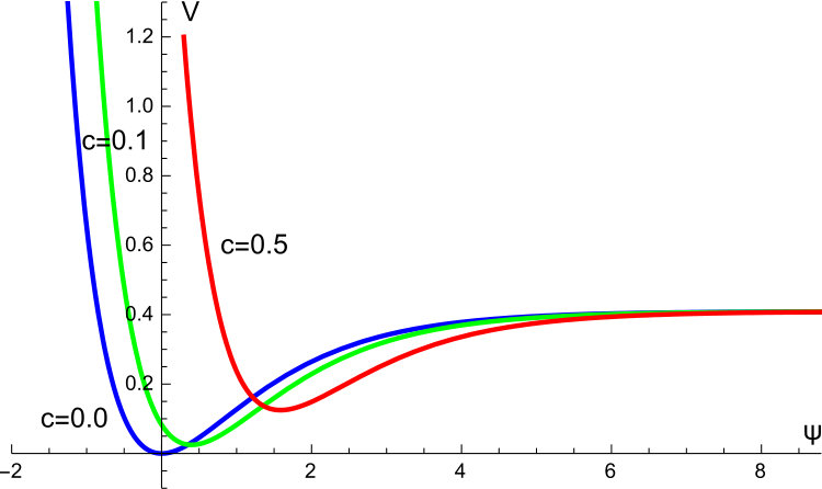 Figure 1
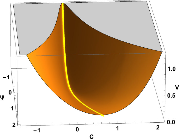 Figure 2
Peer Reviews
No public reviews on file for this paper yet. If you reviewed it on a platform where reviews are public (OpenReview, ICLR, NeurIPS, ICML), you can paste yours below so the community can read it here.
Videos
No videos yet. Explain this paper in a talk, walkthrough, or lecture? Add one.
Deforming the Starobinsky model in ghost-free higher derivative supergravities
*Dedicated to the memory of Peggy Kouroumalou, colleague and friend *
G. A. Diamandis 111email: [email protected], B. C. Georgalas222email: [email protected], K. Kaskavelis333email: [email protected],
A. B. Lahanas 444email: [email protected] and G. Pavlopoulos555email: [email protected]
National and Kapodistrian University of Athens, Department of Physics,
Nuclear and Particle Physics Section, GR–157 71 Athens, Greece
Abstract
We consider higher derivative supergravities that are dual to ghost-free supergravity theories in the Einstein frame. The duality is implemented by deforming the Kähler function, and/or the superpotential, to include nonlinear dependences on chiral fields that in other approaches play the role of the Lagrange multipliers employed to establish this duality. These models are of the no-scale type, and in the minimal case, require the presence of four chiral multiplets, with a Kähler potential having the structure of the coset manifold. In the standard supergravity formulation, these models are described by a multifield scalar potential, featuring Starobinsky-like behavior in particular directions.
Keywords: Supergravity, Modified Theories of Gravity, Inflationary Universe
PACS: 04.65.+e, 04.50.Kd, 98.80.Cq
I Introduction
The study of generalizations of Einstein gravity, considering higher order curvature terms, has a long standing history, for various reasons, related to either cosmology, or towards the effort for understanding the ultraviolet behavior of gravity at the quantum level. The recent activity on this field is mainly motivated by Starobinsky’s model of inflation STAR and, in particular, by the fact that the inflaton may have a “dual” description as the extra scalar mode propagating in a theory stelle ; whitt . Strictly speaking it is proven that this theory is equivalent to Einstein gravity specifically coupled to a scalar field. Going beyond the , general -theories have been studied, see for instance CAPO ; SOTIRIOU and references therein, which are known to be equivalent to the Einstein-Hilbert action, if one introduces additional auxiliary fields which couple to curvature in the Jordan frame. By appropriate Weyl rescalings the Jordan theory is brought to the Einstein-Hilbert Lagrangian with the auxiliary fields becoming dynamical. Also some classes of gravity theories, whose Lagrangians are not only functions of the curvature but may include terms, had been considered in the past. These higher derivative gravity theories have been proven to be equivalent to the Einstein-Hilbert action with additional scalar fields wands . In another context, higher derivative gravities have been invoked against improving the UV (Ultraviolet) behavior of gravity theories, but they suffer, in general, by the presence of negative norm states. This issue has been analyzed in literature, where general gravity actions were considered, involving terms at most quadratic in the Riemmann tensor, in an effort to obtain better UV-behavior and avoid having negative norm states GHOST ; BISWAS1 ; BISWAS2 . Further attempts towards constructing finite and ghost-free, nonlocal MOD1 and local MOD2 gravity theories have been also considered.
Minimal supergravity theories, CREMMER ; BAGGER , being the supersymmetric completion of the Einstein theory, have also been extensively studied in the last forty years or so, in an effort to encompass all of the known forces of Nature, including gravity, into a unified framework. On the other hand the supersymmetric completion of gravity, pertinent to cosmological inflation, is a notable paradigm of how a dual description of the supersymmetric Einstein-Hilbert action can be accomplished. Driven by these, there is a strong motivation towards studying supersymmetric completion of general -theories, going beyond the simple model. The organization of Lagrangians involving higher powers and derivatives of the scalar curvature has been addressed in the past. The minimal theories were considered in THEISEN ; CECOTTI , which were shown to be equivalent to standard supergravity coupled to two chiral supermultiplets. Besides, in CECOTTI a general methodology was developed in order to include arbitrary powers of the scalar curvature as well, which is accomplished using a set of chiral fields that play the role of Lagrange multipliers. In these approaches the dual supersymmetric -theories are equivalent to standard supergravity theories with Kähler potentials of the no-scale type NOSCA ; EKN . The main problem in adopting the full equivalence between the two descriptions, that is the higher- and the standard supergravity, in the case the former departs from the minimal theory, is that while in the higher- description there are no propagating ghost states at the linearised level. This is not the case in the dual description due to the specific form of the Kähler function employed to implement the duality.
Recently there has been an intense activity towards building models that encompass cosmological inflation, especially after the precise data on the cosmological parameters delivered by Planck and other collaborations PLANCK ; BICEP ; PLANCK2 ; BICEPPLANCK . The physics of inflation will be placed under further scrutiny, in the next round of measurements, and this led many authors to consider various models, with or without supersymmetry, KALLOSHX ; KETOV1 ; KETOV ; ELLISp1 ; KALLOSHp1 ; SFERRARA2 ; KALLOSH ; SFERRARA ; ELLIS ; KEHAGIASp1 ; KEHAGIAS2 ; DALIAN ; SCALISI ; ZWIR ; PALLIS ; KOUNNAS ; KTAL ; BUCH ; ANTODUDAS ; ovrut1 ; DGKKLP ; SAGNIOTTI ; teradax ; YAMADA ; ASAK ; KOSHE . In this context supergravity and higher derivative supergravities may play a central role.
In this work we consider chiral higher derivative supergravities that are dual to ghost-free supergravities. This is done by deforming the Lagrangian to include nonlinear dependences, on some of the would be Lagrange multipliers used in the approach described in CECOTTI , which in this way become dynamical. Interestingly enough, even in the simple cases considered, this approach leads, in turn, to scalar potentials which in particular directions have a Starobinsky-like form.
This paper is parametrized as follows. In the following section we review the general set-up for the formulation of supergravity chiral actions, which is an essential tool towards building -supergravity theories, and establish their duality to the standard supergravity description. This approach uses a set of chiral fields, that appear linearly in the action, and play the role of Lagrange multipliers. In Sec. III we apply this formalism focusing on theories that involve at most two derivatives of the curvature , and discuss the problem associated with the ghost issue. In Sec. IV we proceed to a particular deformation of the model by promoting one of the Lagrange multipliers to a dynamical field, which therefore is not eliminated any longer from the action. This is necessary in order to avoid ghosts in the ordinary description of the supergravity. Deforming the theory in this way adds extra difficulty, in expressing the theory in chiral form, and the way this is implemented is discussed in detail. Particular models are presented in Sec. V, whose Kähler potential is reminiscent of the no-scale type. In Sec. VI we analyze the mass spectrum of these models, and in Sec. VII we consider their corresponding supergravity description, in the Einstein frame, and show that the scalars, in a suitable superfield basis, destabilize a coset space. Their mass spectrum has no ghosts and exactly matches that of the dual theory, derived in the previous section. Moreover we show that the scalar potential of the standard supergravity Lagrangian is positive definite with a Minkowski vacuum with unbroken supersymmetry. This potential is described by four complex scalar fields and in particular directions is reminiscent of the well-known Starobinsky model. It is for this reason that we have dubbed the class of models considered in this work as deformed Starobinsky models, although we are aware that the virtues of the single - field Starobinsky model, as far as cosmological inflation is concerned, are hard to obtain. Models of this type can only lead to behavior inflation, and the presence of additional scalars may stabilize the Starobinsky inflationary trajectory. Recently addazi , extensions of the theory, in the framework of the old-minimal supergravity, were considered which are ghost-free, with one scalar field present and a stable potential. A detailed analysis on the cosmological consequences of the class of models discussed in this work is not pursued here, and it will be presented in a forthcoming publication.
II Chiral Lagrangians
In the absence of gauge fields and using superfield formalism, the Supergravity (SUGRA) Lagrangian is written as
[TABLE]
In this denotes collectively all chiral multiplets involved, which are coupled to gravity, and their corresponding anti-chiral multiplets. The kinetic function is real and the superpotential is a holomorphic function . This Lagrangian, expressed in terms of components, is a function of a Kähler function, given below, and its derivatives,
[TABLE]
In this the Kähler function is related to by
[TABLE]
The above Lagrangian can be cast in the so called chiral form
[TABLE]
This is particularly useful since any supergravity action can be written as a chiral action which includes chiral multiplets and their corresponding kinetic multiplets ! We shall make extensive use of this form when dealing with higher supergravities.
In a previous paper DLT we considered minimizavities whose construction is implemented using chiral multiplets coupled to gravity. The gravity sector itself is well-known to be described by the chiral superspace density , the supervierbein determinant , and the chiral superspace curvature . Ignoring their fermionic components, and are given by
[TABLE]
where and are the auxiliary fields of the gravity multiplet. 666 Throughout this paper, the metric signature is and the sign of the scalar curvature coincides with that used in CREMMER .
In superfield formalism, omitting fermions, a Poincaré chiral multiplet is written as
[TABLE]
Given a chiral multiplet , another chiral multiplet can be constructed whose scalar component includes , that is the complex conjugate of . This is called kinetic multiplet and is given by 777 This is times the corresponding multiplet used in reference BAGGER .
[TABLE]
In this is the ordinary gravity d’ Alembertian operator, i.e. . This multiplet can be expressed as the chiral projection of the anti-chiral field ,
[TABLE]
With this definition the kinetic multiplet of the unit chiral multiplet is twice the curvature multiplet, i.e.
[TABLE]
while the kinetic multiplet of the curvature chiral multiplet is given by
[TABLE]
Later, we shall use the kinetic multiplet of which, in a straightforward manner, is found to be
[TABLE]
Note that this includes and within its -term. These forms are the important building blocks towards building -supergravity theories, as we shall see.
One can build actions involving the chiral multiplets , , , and so on, as well as other chiral multiplets, which we denote collectively by . Thus one may consider Lagrangians having the general form,
[TABLE]
Such Lagrangians describe higher theories, by construction, and these are equivalent to standard supergravities, in which only the Einstein term appears CECOTTI . In fact by introducing Lagrange multipliers, , one can show that (12) is equivalent to a standard supergravity described by the following functions,
[TABLE]
In these neither nor depend on . The theory described by is then written as
[TABLE]
where is the part of the Lagrangian dependent on the Lagrange multipliers, appearing in the function and the superpotential given before in Eq. (13),
[TABLE]
In deriving this, repeated use was made of the very important relation
[TABLE]
which holds true, up to four divergences, for any chiral multiplets . Its derivation is almost straightforward, using the equivalence of the Lagrangians (1) and (4) and employing (8). Solving with respect the Lagrange multipliers we get
[TABLE]
Plugging the solutions into (14) yields exactly (12), due to the fact that vanishes. This proves the equivalence of the two theories.
As an instructive well-known example consider the no-scale supergravity CECOTTI ; KETOV ; KALLOSHp1 ; ELLISp1 ; SFERRARA2 model described by
[TABLE]
One sees that in this case we have one Lagrange multiplier , which equals to in this case, while is identified with . The functions are given by
[TABLE]
The Lagrangian (15) is, in this case, given by
[TABLE]
and the total Lagrangian, cast in chiral form, is
[TABLE]
The equation of motion for , , is
[TABLE]
which when plugged into the Lagrangian (21) eliminates the last term, which is proportional to , leaving
[TABLE]
Using the explicit forms of , given previously, this trivially leads to the following Lagrangian, also derived in DLT using the component formalism,
[TABLE]
Note that the scalar is linearly related to the scalar component of the superfield , on account of (22). In fact . The term arises from the first term of (23) and the linear term from the second term of the same Lagrangian. 888 Modulo stabilization terms, introduced to stabilize the inflationary trajectory, Eq. (24) is the one obtained in addazi when is replaced by , used in that work, and the constant of that paper is taken vanishing.
This is the dual form of the ordinary supergravity Lagrangian specified by given in (18) . The bosonic part of the latter depends on scalars and is linear in the curvature , describing therefore six degrees of freedom (d.o.f.), the same as (24). Along the direction this receives a simple form
[TABLE]
If is frozen to , then by defining a canonically normalized field , by , we get
[TABLE]
which is the celebrated Starobinsky’s model STAR ; whitt , with being the inflaton field with the parameter setting the scale of inflation.
III Higher derivative theories
The strategy outlined in the previous section can be employed to construct higher derivative supergravity theories. The supersymmetric Starobinsky model includes terms at most quadratic in the curvature . Using two Lagrange multipliers we can build a higher derivative -theory, as follows. Consider the theory described by
[TABLE]
The correspondence with the previous notation, if needed, is given by
[TABLE]
The functions do not involve, at this stage, any of the Lagrange multipliers . Treating the Lagrange multipliers as described in the previous section, the Lagrangian corresponding to this theory has the following form,
[TABLE]
This is easily solved for the Lagrange multipliers ,
[TABLE]
With plugged into (29) we get
[TABLE]
We remark that using only two Lagrange multipliers is sufficient to build higher- supergravities. This is the most economic way and in the rest of this work we shall not pursue more complicated cases involving a larger number of them.
In order to implement this, consider, as an example, the simple case of having a theory specified by
[TABLE]
According to (31) this theory is
[TABLE]
where in the last step we put the Lagrangian in chiral form as prescribed in the previous section. This is a higher- theory. In order to show this, collect the terms that depend only on the curvature, after integrating over . The result is
[TABLE]
which is indeed a higher theory.
However it should be noted that in the ordinary supergravity form, the theory described by (27) is linear in , and ghosts exist that are not present in the dual description (33). The appearance of ghost states becomes manifest by the fact that some of the eigenvalues of the complex scalar kinetic matrix are negative. On the other hand counting the degrees of freedom of the two theories there is a mismatch. The dual theory appears with fewer degrees of freedom as compared to the ordinary supergravity and no ghosts at all. Obviously the ghost states of supergravity should decouple, in some manner, since the number of physical degrees of freedom in both descriptions should be equal. A way to implement the ghost decoupling, in some particular cases, was given in DLT . Here we shall pursue an alternative way by constructing theories that have no ghosts in their formulation. This is merely done by sacrificing the role of the field as being a Lagrange multiplier. In doing that, the field becomes dynamical and is no longer eliminated, and then the degrees of freedom in the two descriptions match. In the following section we shall give the details of how this is implemented and chiral actions of this kind can be constructed.
IV - Deformations
A way to circumvent the ghost problem, outlined in the closing remarks of the previous section, is to deform the theory so that the functions and or in Eq. (27) depend on the Lagrange multiplier . As we already remarked this may rectify the situation and no ghost states appear in the standard formulation of the supergravity.
In order to tackle the problem in the most general manner let us consider theories in which the functions are given by
[TABLE]
These are like (27), however, the functions are now allowed to have dependencies. Evidently the dependence on the superfield is not linear any longer, and hence, is not eliminated from the action.
We shall assume the most general form for the function which when expanded in powers of the chiral superfields , and their associated anti-chiral fields , it receives the form
[TABLE]
Using (16) this can be written as
[TABLE]
where the sum extends over the monomials
[TABLE]
With that done the Lagrangian can be put in chiral form
[TABLE]
with the superpotential function given by
[TABLE]
Denoting for convenience
[TABLE]
any superfield variation of the action, where is any of , yields
[TABLE]
In the last step we used the fact that
[TABLE]
which holds true up to four divergences. Therefore the equations of motion for , in superfield form, are given by
[TABLE]
In order to proceed further let us consider a specific function given by
[TABLE]
where the constants are assumed positive. The function in Eq. (45) ensures that the standard supergravity theory has a positive kinetic function in the sector , under the condition , and therefore no ghosts appear ! For the case at hand the following terms are encountered in the sum of Eq. (37) with the terms given, respectively, by
[TABLE]
In the following we assume, for simplicity, that there is no dependence of the superpotential function . Also, we assume that no additional multiplets are present. These can be added in a trivial manner later, if desired. Then the equations of motion for the superfields , using equation (44) and the form of given by Eq. (41), yield
[TABLE]
Solving for and plugging into the function , given in Eq. (40), one arrives at
[TABLE]
In this are solved by (47), that is they are given by
[TABLE]
We see that the field , unlike , is no longer eliminated and was not expected to. The independent chiral multiplets are and the Lagrangian is expressed in terms of these, and kinetic multiplets that follow from these chiral superfields. Actually, from Eqs. (39) and (40) we find that the resulting chiral Lagrangian has the form,
[TABLE]
where it is meant that the arguments within are replaced by the solutions given in (49). This is certainly a higher -supergravity. In fact we have seen from (33) and (34), that the term leads to
[TABLE]
where the ellipsis denote additional terms that either mix with other fields or they do not depend on the curvature at all. Note the appearance of the term which is unavoidable due to the appearance of the term in the definition of the function , see Eq. (45). Note also the appearance of the term , encountered also in the Starobinsky action (23), which yields, see (24),
[TABLE]
However this does not exhaust all possibilities and the presence of the superpotential function in Eq. (50) is source of additional -dependent terms yielding higher- supergravities. In the following section, we shall consider particular choices for the function , some of which are generalizations of the Starobinsky model.
V Building -Supergravities
In this section we shall consider specific models, whose the pertinent functions are as given in (35), with the function defined by (45). The function assumed to depend only on , that is the superpotential part has no -dependence. As we shall see the deviation from the -linearity, existing in the function , induces deformations of the Starobinsky model for properly chosen functions .
From Eqs. (49) we have for the scalar components and the corresponding -terms, of the chiral fields
[TABLE]
In these stand for the scalar component and the -term of the chiral multiplet . The solutions for the components of the multiplet is much easier to handle since is just , yielding
[TABLE]
The Lagrangian (50) involves terms that are products of two multiplets and thus we can make use of the general result
[TABLE]
This is easily derived, ignoring the fermionic contributions. are any two chiral multiplets, whose scalar components are denoted by the lower case letters , while their -terms are denoted by respectively.
V.1 Models with
Let us first consider a simple model in which the superpotential part involves a general function of the multiplet , that is
[TABLE]
In this case, writing the multiplet as , the function receives the form
[TABLE]
Then using (56), taking one of the multiplets to be the unit multiplet, we easily get for the -dependent part of the Lagrangian,
[TABLE]
Using (53) and (54), and collecting the terms in and that depend only on the curvature , we get,
[TABLE]
In this is the scalar component of . Evidently this does not contain pure curvature dependent terms. It involves terms in which the curvature mixes with other fields, namely in this case. The same holds for the remaining terms of that we have not shown. As we shall see, in the Lagrangian (50) all fields are dynamical, even . Therefore cannot be expressed in terms of other fields and (60) cannot lead to a Lagrangian depending exclusively on the curvature . Therefore this choice for the superpotential leads to a dual supergravity description whose pure -terms are only those presented in (51), (52). Obviously one needs to depart from this type of superpotential in order to build dual supergravities involving higher powers of the curvature, other than those given in (51), (52).
V.2 Models with
From the previous discussion we have seen that the function should involve, besides the dependence on , dependence on the superfield as well, in order to construct a general -supergravity. An interesting case arises when is linear in the superfield having the form
[TABLE]
Interestingly enough this choice leads to generalizations of the supersymmetric Starobinsky model. We shall term these as “deformed” Starobinsky models. In order to see this, and to make contact with the usual notation found in literature, we rescale the fields and fields by
[TABLE]
Then the functions given in (35), with defined by (45) and the function given by (61), take the following forms
[TABLE]
where . The function gives rise to a Kähler potential having the structure of the no-scale models. The symmetries of the associated Kählerian manifold will be discussed later. The first terms of above, depending on , are the ones encountered in (18), the supersymmetric Starobinsky model. As we shall see later, the standard supergravity description of this model has a Starobinsky-like potential along a particular direction. However the scale of the scalar potential of the inflaton field is not , although it is related to it. We shall come to this point later.
The class of models just discussed are higher -supergravities in their dual description. The presence of and kinetic terms in , which are necessary in order to ensure absence of ghost states in the standard supergravity description, induces terms higher than encountered in the simple Starobinsky model. Actually, we have already seen that terms are induced, see Eq.( 51), due to the appearance of the term in . However the presence of a nontrivial superpotential part , as given above, gives rise to additional curvature dependent terms leading to more general -supergravities.
In order to find the curvature dependent terms, stemming from , we shall consider in (61) to be an arbitrary function of the chiral field . In this case the chiral form of the superpotential is
[TABLE]
so that, in this case, we get from the -dependent part of the Lagrangian given in (50)
[TABLE]
Replacing in this the solutions (53) to (55) we get, in a straightforward manner, the -dependent part of the Lagrangian which is given by,
[TABLE]
In this it is meant, without saying, that the scalar field , appearing within both , is expressed in terms of other fields using the solution (53). Putting we get the result derived in DLT , see Eq. (45) in this reference. However is mandatory in order to have an Einstein supergravity without ghosts, as we have already remarked. If we keep the terms that depend only on the curvature , in the above Lagrangian, and adding the corresponding curvature dependent contributions from (51), (52) we arrive at
[TABLE]
In this, for convenience, we have taken to be real function when its argument is real. The ellipsis denotes additional terms, among them curvature dependent terms which however mix with other fields. The Lagrangian (67) is indeed a -supergravity whose precise form is specified by the choice of the function . For the simple choice , which eliminates the last term in the superpotential given in Eq. (63), the deformed Starobinsky model leads to
[TABLE]
For the complete form of the Lagrangian one should also add to (67) the terms from Eq. (50) that depend on the chiral multiplet . These do not contribute to terms that depend solely on the curvature . However they are essential for studying the mass spectrum of the dual theory. This task will be undertaken in the following section.
VI The mass spectrum of the dual -theory
The mass spectrum of the dual theory can be read by isolating the bilinear terms in the Lagrangian (50). To that purpose, we shall pick the quadratic in the fields terms, separately for each term appearing within (50), keeping however the complete expressions for those terms that depend exclusively on the curvature .
Using previous results, see Eqs. (23) and (24), from the term we get
[TABLE]
This is the complete expression. Collecting the quadratic terms, with the exception of the terms that are only -dependent, as we have already remarked, we get
[TABLE]
For the term in the Lagrangian (50) having the structure
[TABLE]
the quadratic pieces are given by
[TABLE]
For the term which mixes with , namely
[TABLE]
the quadratic terms are given by
[TABLE]
As for the terms that depend on the multiplet , the term
[TABLE]
yields a quadratic piece given by
[TABLE]
while the term
[TABLE]
gives rise to quadratic terms given by
[TABLE]
Note that the fields in the dual description, unlike the Einstein frame supergravity, are no longer auxiliary and hence cannot be eliminated ! This is intimately related to the fact that nonlinear terms were introduced. Therefore, the deformed theory has additional dynamical d.o.f., as compared to a theory in which appears linearly, and thus it comes closer to having the same number of d.o.f. with the ordinary supergravity in the Einstein frame. In fact, there is no mismatch in the number of d.o.f., as we shall see., which is a welcome feature signaling the absence of ghosts in the standard supergravity description.
It only remains to read the quadratic part of the Lagrangian (66) which can be implemented by expanding the function . By a straightforward calculation one finds, recalling that the function has been taken real for real values of ,
[TABLE]
In the last step we should collect all quadratic terms, given so far, in order to read the mass spectrum of this dual theory. This may not be as easy due to field mixings occurring in the Lagrangian. In doing so it proves easier to use the real and imaginary components of the fields involved as follows
[TABLE]
The longitudinal component of the field we have denoted by . With these definitions the quadratic part of the total Lagrangian is given by
[TABLE]
The function includes all terms, even nonquadratic, that depend exclusively on the curvature, but not on its derivatives. Its specific form is given by,
[TABLE]
The constants appearing in (81) stand for and respectively. Since the real function is arbitrary so is the function and hence the constants . Expanding the function , the linear in the curvature term is
[TABLE]
This dominates in the weak field limit but is not a canonically diagonalized Einstein term . However this can be remedied by an appropriate constant rescaling of the metric, , with , which brings the curvature term in (83) to its well-known Einstein form .
The fields get mixed in the bilinear terms therefore the mass spectrum is rather difficult to read directly at this stage. Note, especially, the mixing of the curvature with the real part of the field , denoted by . As has been already discussed, is dynamical in this formulation since the Lagrangian includes derivatives of it. Isolating the bilinear terms involving the curvature and the field , and rescaling the field , by , so that its kinetic term is canonical, we get
[TABLE]
The simplest way to derive the tree-level mass spectrum is to find the equations of motion of all fields involved. For the Lagrangian (84) the equations of motion that follow by varying the metric and are given below. The variations of each term in Eq. (84), with respect to the metric, are presented in Appendix A. It is essential to note that only the linear terms will be kept in the equations of motion, since we want to find the tree-level mass spectrum, which makes the task much easier. Then for the variations , given in Eqs. (170) - (173), we pick only the linear terms. Then employing the fact that , which follows from Eq. (82), we arrive at
[TABLE]
Then we expand in the usual manner around the flat metric , that is . Then, by defining the field , see (175), and employing the harmonic gauge, (176), the equation of motion receives the following form
[TABLE]
The parameters appearing in this equation depend on and as can be seen from Eq. (82). The precise relations are given in (183). As for the equation of motion that follows by varying the field , this is much easier to be derived leading to
[TABLE]
Keeping the linear terms in , and in the harmonic gauge, this receives the form
[TABLE]
where . Eqs. (86) and (88) can be written as
[TABLE]
where for convenience we have denoted . The constants , as well as , can be read from (86) and (88). Eq. (90) can be plugged into (89) yielding
[TABLE]
This contracted with the flat metric yields
[TABLE]
Solving (90) , (92) we get a system of two coupled Klein-Gordon equations,
[TABLE]
The constants appearing in this equations can be read from the previous expressions. Note that the “off-diagonal” coefficients are not equal. This system can lead to two uncoupled Klein-Gordon equations by linearly combining . In order to implement this we write the above system as
[TABLE]
The system (100) can be uncoupled by a real matrix that diagonalizes ,
[TABLE]
where are the eigenvalues of . Then the “rotated” fields defined by
[TABLE]
are two independent Klein-Gordon fields satisfying
[TABLE]
The masses squared are the eigenvalues of the mass matrix defined in (100). They are explicitly given in Appendix C, see (181), where we also discuss the conditions for them to be real and nontachyonic.
The graviton field is given by
[TABLE]
Since is transverse so is that is, , and it satisfies the massless Klein-Gordon equation, as can be seen by acting with the operator on ,
[TABLE]
if the constants are given by
[TABLE]
To arrive at (111), Eqs. (91) and (109), as well as (108) , were used. Therefore the physical degrees of freedom of the sector are a massless graviton and two massive scalars with masses given in (181).
As for the remaining degrees of freedom, consider the field , which mixes only with the imaginary part of named , in the bilinear terms. The equations of motion are fairly easy to be derived. In particular by varying with respect one gets
[TABLE]
from which, acting upon it by , we get
[TABLE]
On the other hand the variation with respect yields,
[TABLE]
Plugging the left hand side of (115) into (114) and by defining , for convenience, we get the system of equations
[TABLE]
The constants appearing in this equations can be read from previous expressions. The “off-diagonal” coefficients of the mass matrix are not equal, in general. However, this system also leads to two independent Klein-Gordon equations, if one diagonalizes the matrix by a real matrix, as we did in the previous case, see (103). The corresponding masses squared are the eigenvalues of the mass matrix appearing on the right of (122). They are analytically given in (191) where it is shown that they are identical to the masses (180). The reason behind this degeneracy will be discussed later.
It remains to find the equations of motion for the system of the fields and . It is seen from Eq. (81) that and are coupled, but do not mix with which are also coupled. Note that the pertinent Lagrangian terms for the system follow exactly from those of by replacing and . Therefore it suffices to study one of these systems. The equations of motion that follow from (81), by varying and respectively, are given below
[TABLE]
By defining the combination
[TABLE]
and using this to replace in the equations above the field in terms of we get, combining the resulting equations,
[TABLE]
The constants can be read from Eqs. (123) and (124) and are given in (192). Acting in the first of (126) by and replacing in the resulting equation by the second of (126), we get a system which in matrix notation has the following form,
[TABLE]
The mixing matrix is not symmetric, in general. Its elements are explicitly given in (193). Diagonalizing this, we get two Klein-Gordon equations for some linear combinations of . The relevant masses squared are the eigenvalues of the matrix above. These are found to be identical to (187), and hence (180). For a proof see discussion following (192). The system of has exactly the same mass spectrum as the system, as we have discussed.
Before closing this section, we should point out that the masses derived in this section are in a frame in which the linear in the curvature term is , see Eq. (83). However masses are usually quoted in the Einstein frame in which the curvature term is normalized to . As already pointed out, this can be implemented in a trivial manner with a constant rescaling of the metric [ see discussion following Eq. (83) ]. The effect of this is that the masses derived in this section should be multiplied by the factor to derive those in the Einstein frame, which enter Newton’s law.
To conclude, the mass spectrum consists of a massless graviton, four scalar degrees of freedom of mass and another four scalars with masses , given analytically in (181). The reason for the resulting mass degeneracy, in this simple model, will be discussed when dealing with the standard supergravity in the Einstein frame, whose spectrum should coincide with this of the dual theory considered in this section. This task will be undertaken in the following section.
VII Supergravity
The previously defined models are dual descriptions of standard supergravities where the curvature term has its canonical Einstein form, . In this frame the kinetic and potential terms of the theory are given by
[TABLE]
In these denote respectively the scalar fields involved, and their complex conjugates, and . The -terms are given by
[TABLE]
As usual, the subscripts denote differentiation with respect and is the inverse of the kinetic matrix .
For the class of models studied in the previous section, the superpotential is
[TABLE]
with an arbitrary chiral function of , and the Kähler function is related to the real function as given in (3). The latter is given by
[TABLE]
The complete form of the scalar kinetic part is rather lengthy and will not be presented. However it takes a rather simple form if we keep the bilinear parts in the fields, and their conjugates, by expanding about preserving the terms that depend on . The reason behind this expansion relies on the fact that the point , as we shall see shortly, corresponds to a global minimum of the scalar potential. In this expansion the kinetic terms are,
[TABLE]
where the first two terms are the ones encountered in the Starobinsky model. Instead of using we can define a real scalar field by
[TABLE]
The choice of the pre-factor of the exponential in (140) is not essential since by shifting the field can be changed to anything. However this choice is convenient since, as we shall discuss, the minimum of the potential lies at , or same . With this definition the kinetic terms given in (139) receive the following form
[TABLE]
Expanding the exponentials about the point , anticipating the fact that at the minimum , we get
[TABLE]
These kinetic terms are not canonically normalized. Moreover they mix in the sector. The kinetic mixing matrix associated with the sector has determinant proportional to . Therefore when either or vanish, that is when there are no diagonal quadratic kinetic terms for either or fields, one of its eigenvalues is negative. This signals the appearance of ghost states ! Taking all eigenvalues of the kinetic mass matrix in (142) are positive definite and this is a necessary condition in order to avoid ghosts. Note that this condition lies in the range where the mass squared of the dual theory are positive definite, see Eq. (186).
Having discussed the kinetic part we now move on to study the scalar potential. The complete potential has the following form,
[TABLE]
The first three terms are manifestly positive definite. The last two are not and the potential in not bounded from below. Additional terms need be introduced to stabilize the scalar potential, as the ones employed in EKN ; KALLOSHp1 . Adding a single stabilizing term KALLOSHp1
[TABLE]
to the function is adequate to stabilize the scalar potential as we will discuss. That done, the scalar potential receives a rather complicated form, which, however, we can handle analytically. Its complete expression is given by (196) and (197). In Appendix D we discuss in detail its minima and its stability. In fact we find that the potential has a minimum at the point
[TABLE]
As we show in Appendix (D) there are values of for which the potential is positive definite for any value of the fields involved. Therefore this minimum is actually the absolute minimum of the potential. At the minimization point (145) the scalar potential vanishes, see (201), that is we have a Minkowski vacuum. Moreover at this vacuum supersymmetry remains unbroken, since for any value of .
Being the absolute minimum, the matrix of the second derivatives, at this point, should be positive, i.e. all of its eigenvalues should be positive definite. This statement is equivalent to saying that there are no tachyonic masses in the spectrum of scalars, which we shall prove in the following. We point out that the mass spectrum is independent of the stabilizer. Actually, expanding the potential about the point (145) its quadratic terms do not depend on as can be seen from the form of the potential, given in (196), using the fact that at the minimum (201) holds. This differs from other supergravity models, in which the scalaron has a -dependent mass due to the fact that the lowest minimum of the potential is -dependent, as well addazi .
In fact by expressing the fields in terms of their real and imaginary parts, and trading for the field , defined in Eq. (140), we find that the quadratic terms arising from the potential are given by
[TABLE]
In it the constants are given by
[TABLE]
In (146) the fields are mixed pairwise. In fact mixes with , mixes with , mixes with and mixes with . Having the bilinear kinetic and potential terms it is fairly easy to find the mass spectrum. This task is facilitated a great deal by the fact that the mixings among the fields are done in a pairwise manner and we only have to generalize two by two matrices. Due care should be taken by the fact that in the kinetic part the fields are not canonically normalized and, besides, mixings occur in the sector, as is evident from (142). That done we find that the masses are exactly the same with the ones derived in the dual theory if the latter are multiplied by a factor . The origin of this difference was adequately explained in the concluding remarks of the previous section, and is due to the fact that masses read in the Einstein frame differ by a constant from those in other frames in which the curvature term appears with a different normalization.
An alternative, and perhaps more elegant way, to deal with the mass spectrum, and also shed light to the issue of mass degeneracy, is to change the superfield basis. Concerning the mass degeneracy, a double mass degeneracy is expected among the scalars due to supersymmetry that is not broken at the minimum of the potential. Scalar degrees of freedom have same masses with their fermionic counterparts, the latter occurring in two helicity states. Therefore, to each Weyl fermion, there corresponds two real scalar fields having the same mass. However a larger mass degeneracy is observed, actually twice the one expected. In order to treat the system in a more symmetric manner and find the source of the degeneracy, we had better change the superfield basis, working instead with shifted fields, defined by
[TABLE]
These shifts are dictated by the form of the superpotential (137), when its last term is expanded in powers of , which in this way receives the following form,
[TABLE]
The last term in the expression above is at least cubic in the superfields involved and will not actually concern us. The kinetic function given in Eq. (138) can then be expressed in terms of the new multiplets. To that purpose, it proves easier to use a rescaled field, . Within mixings of occur, and by a suitable orthogonal rotation of the superfields these can be uncoupled
[TABLE]
leading to the following functions,
[TABLE]
To cast these functions as above, we have also implemented the following trivial rescalings
[TABLE]
where are exactly the masses given in Eq. (181). The last term in the superpotential is a function of which is at least cubic in the superfields. This will not be explicitly shown, since will not concern us for the discussion that follows. It suffices to say that it has the form with a function at least quadratic in the superfield . The advantage of working with the basis of superfields is twofold. The first is that the function is brought to a form corresponding to a Kähler potential whose scalar fields parametrize the coset space . Such a parametrization is a general feature of the no-scale models. The scalar kinetic terms are those of a nonlinear sigma model having as isometry group the noncompact symmetry. The second reason is that, the scalar fields corresponding to the multiplets have vanishing values at the absolute minimum of the potential, which, as we have already said, is a Minkowski vacuum with unbroken supersymmetry. This, in conjunction with the fact that the superpotential is at least quadratic in the fields, has the effect that the only quadratic terms of the potential, when it is expanded about its Minkowski vacuum, are those stemming from the -terms. In particular, one needs only to calculate the derivatives of the first terms in the superpotential given in Eq. (159), and the last term plays no role in the mass spectrum. This facilitates the calculation a great deal, in both identifying the scalar mass eigenstates, and find the mass spectrum, and also tracing the source of the mass degeneracy. In particular, in this basis the Kähler metric, and its inverse, receive a simple diagonal form, at the minimum,
[TABLE]
and thus the quadratic terms of the potential are given by
[TABLE]
In this and are the scalars of the multiplets respectively, while are those of the rotated multiplets defined by and . Note that are exactly the combinations of multiplets appearing in the first part of the superpotential given in Eq. (159). As for the kinetic terms, collecting the quadratic terms, using the fact that the Kähler metric in the basis is diagonal having the simple form (161), we get, after replacing the scalars by ,
[TABLE]
From Eqs. (162) and (163) we see that have common masses squared and have , with given in (181). This we have already found previously in an alternative manner.
Note that by working in the new basis not only the scalar sector is treated more symmetrically, but also the flat limit, , is more easily obtained. In fact, modulo normalization, the scalar kinetic and the mass terms given before are those encountered in a globally supersymmetric model involving four chiral multiplets. In particular, in the flat limit only renormalizable couplings survive, and the model smoothly goes to that of a a rigid supersymmetry with four (normalized) chiral fields, given by
[TABLE]
and a superpotential
[TABLE]
In this, are the rescaled masses , and in this limit only the renormalizable cubic terms have been kept in the -term appearing in Eq. (159), designated as “cubic terms” in Eq (165). The scalar potential of the theory is that of a global supersymmetry, having the well-known form
[TABLE]
whose vacuum does not break supersymmetry. Then, from this form it is evident that to each multiplet pair their corresponding complex scalars, i.e., four degrees of freedom, have common masses appearing in the superpotential . This degeneracy is due to the specific choice for the superpotential, given in (165), whose only mass terms are those mixing , with a mass parameter , in the way shown above. Had we included the fermionic components we would have found that the fermionic Weyl components of multiplets also mix in their mass terms, exactly in the same manner, with a mass parameter . Therefore they compose the left- and right-handed components of a Dirac fermion having mass . Thus, we have four fermionic degrees of freedom, of mass , which exactly match the bosonic degrees of freedom, as expected in unbroken supersymmetry.
Having found the complete form of the potential, and in order to have a better understanding of its behavior, we start from its absolute minimum and move in the direction, keeping the remaining fields to their vacuum values, , see (145) . We then see, from (196) and (197), that it has the simple form,
[TABLE]
Various profiles of the potential are presented in Fig. 1, for some representative choices of the function . In this figure we display the potential as function of , defined in (140) by , for various values of and . In each case shown, the potential has the form of a Starobinsky-like potential whose minima lie higher, for higher values of , the lowest minimum being attained for . The potential as function of and , with the remaining fields set to zero, has a funnel-like shape, as shown in Fig. 2, which narrows as gets smaller. On this curve we have also drawn the trajectory of the minima in the direction for fixed values, i.e. the points corresponding to . The role of this trajectory will be discussed in later.
For vanishing values of the potential (167) takes the simple form,
[TABLE]
which by replacing by the field , using (140), and in the particular direction , it receives the well-known form of the one field Starobinsky potential,
[TABLE]
Its scale is set by a combination of the parameters , as is evident from (169).
Therefore, we have constructed a higher derivative supergravity of the form , whose dual Einstein-Hilbert description has no ghosts and its potential is described by four complex scalar degrees of freedom. This is positive definite, having one stable Minkowski vacuum, with unbroken supersymmetry. Starting from this minimum, and moving in particular directions, the scalar potential has the shape of the well-known Starobinsky model. It is mainly for this reason that we dubbed the class of models described in this work as deformed Starobinsky models. We are aware that the virtues of the single-field Starobinsky model, which successfully describes cosmological inflation in a simple manner, may not be shared by the class of models considered here. In fact the models considered here are unavoidably multiscalar and only in particular directions have profiles reminiscent of the Starobinsky potential. However this by itself is not adequate to reach the conclusion that they are successful in describing cosmological inflation.
A thorough study of the cosmological consequences of these models are beyond the scope of the present paper. However we may present reasons why this class of models may be of relevance for cosmological inflation. Although it is premature to reach definite conclusions, the qualitative features of the potential are such that a two-field inflation may be sustained, in principle. In particular, starting from some initial values of the fields , freezing the remaining degrees of freedom to their vacuum values, the field rolls down to reach the minimum in the -direction, that is it starts tracking the trajectory drawn in Fig. 2. Then the fields , are decreased continuously, in their journey to the absolute minimum, which corresponds to . Although we have verified numerically this behavior, evidently this scenario has to be taken with a grain of salt, as far as its cosmological predictions are concerned, and a thorough investigation will appear in a forthcoming publication. In particular the role of the other fields, that we have frozen at their minimum values, may upset the whole picture since during the evolution the frozen scalar degrees of freedom may depart from their minimum values destabilizing in this way the inflationary trajectory.
Concluding this section, we have seen that the departure from the linearity of the -field, that plays the role of a Lagrange multiplier when it linearly appears in the theory, besides leading to a standard old-minimal supergravity theory free of ghosts, it also yields supergravity models having a no-scale structure, with Kähler potentials describing the coset . These are characterized by a stable scalar potential, described by four complex fields, with a single Minkowski vacuum and unbroken supersymmetry. In particular directions the scalar potential has a Starobinsky-like form. A detailed study of its cosmological consequences will be presented in a forthcoming publication.
VIII Discussion - Conclusions
In this work we have addressed the question whether higher derivative supergravity models can be dual to ordinary ghost-free supergravities. It has been long known that such a duality, for -supergravities, can be established with the aid of two pairs of chiral multiplets, one pair serving as Lagrange multiplier and the other solving in terms of and respectively. The higher derivative supergravities constructed in this manner do not include derivatives of the scalar curvature, while introducing additional multipliers leads to more general theories involving, also, derivative terms etc. CECOTTI . It is also known, that this description suffers from the appearance of ghost states (poltergeists) in the Einstein frame supergravity, which are in general as many as the Lagrange multipliers, which should decouple from the spectrum.
The aforementioned construction can be generalized by modifying the kinetic function so as to include genuine kinetic terms, for the chiral multiplets involved to implement the duality. In this approach we managed to get ghost-free supergravity models, in the Einstein frame, which have dual formulation as higher derivative supergravities. Using the minimal construction, with the least number of chiral fields present, the characteristics of these theories is that in addition to curvature dependent terms, -terms are also present. Besides, since in this formalism one of the Lagrange multiliers is promoted to a dynamical field, the higher derivative supergravity remains coupled to this chiral field which, unlike previous constructions, is not eliminated from the action. In this way the dual theories have the same number of dynamical degrees of freedom. Within this framework we worked out specific examples showing analytically the coincidence of the mass spectrum between the two descriptions and the absence of ghost states.
The construction presented in this work, although it shares features of existing descriptions found in the literature, is different from them in many respects. For instance, auxiliary fields are also present in the case of the constrained superfield formalism ROCEK ; KOMAR ; ANTODUDAS ; KUZENKO ; farakos1 ; farakos2 ; mosk but obviously in our work the fact that they survive in the on-shell Lagrangian is not due to any constraint. It is also known that other higher derivative models, including operators of the form , can lead to a ghost-free theory in four dimensions DudasG ; ovrut1 ; ovrut2 ; ovrut3 . The inclusion of these terms leads to cubic equations for the auxiliary fields of the chiral multiplets, without inducing kinetic terms for them. The solution of these equations, for the elimination of the auxiliary fields, gives three inequivalent on-shell theories. Restrictions from the effective field theory rules out the two of them, leaving only one consistent solution louis . In our approach the couplings of all chiral fields involved, in the higher- description, arise naturally, while in the Einstein frame the model is quite conventional.
The simple higher derivative theories considered in this work lead unforcefully to generalizations of the supersymmetric Starobinsky model, in the supergravity formulation, in the Einstein frame. These models are of the no-scale type, with the associated Kähler function having the structure of the coset manifold. We have presented a preliminary discussion concerning the possibility that the resulting scalar potential of these models can drive cosmological inflation. Recall that in the description of -supergravity in the Einstein frame, although ghosts may decouple from the theory CECOTTI the potentials arising are in general unstable or, in special cases, not obviously leading to inflationary behavior DLT . In the model worked out in this work, the arising potential features interesting properties. It exhibits Starobinsky directions, as in the supersymmetric completion of theory, and besides, no extra instabilities are developed. In particular, although in our case the scalar potential is described by four complex scalar fields, nevertheless introducing a normalizing term KALLOSH is adequate to render the potential stable, exhibiting an absolute Minkowski vacuum that does not break supersymmetry. The cosmological evolution may, in principle, lead to a multifield inflation. We find this case interesting enough to be considered, although additional stabilizing terms, if introduced, may lead to the conventional single-field inflation. A systematic study of the cosmological aspects of this kind of models is under study and the results will appear in a forthcoming publication.
Acknowledgements
This research has been financed by NKUA ( National Kapodistrian University of Athens ). A.B.L. wishes to thank K. Tamvakis and A. Kehagias for illuminating discussions.
Appendix A Variation with respect to the metric
The following variation formulae are useful towards deriving results given in the main text. One finds that
[TABLE]
and also
[TABLE]
Moreover
[TABLE]
and
[TABLE]
Appendix B Expansion about the flat metric
For the expansion about the flat space-time metric, the pertinent formulae are given below.
[TABLE]
and one defines, in the usual manner,
[TABLE]
In the harmonic ( de Donder ) gauge we have
[TABLE]
For the curvature, keeping the linear terms,
[TABLE]
In this is the flat metric d’ Alembertian operator. In the harmonic gauge
[TABLE]
and also ( in harmonic gauge )
[TABLE]
Appendix C Mass spectrum and allowed range of the parameters
The mass spectrum, arising from the mixing of the graviton with the real part of , includes two massless states, the graviton in two helicity states, and two massive Klein-Gordon fields. The masses squared are the eigenvalues of the mass matrix appearing in (100) and hence they are given by
[TABLE]
These should be real and nontachyonic, which restricts the available range of the parameters involved. However there are ranges, as we shall discuss later, where these conditions can be simultaneously satisfied. Their masses squared in (180) can be more conveniently expressed in the following manner,
[TABLE]
In this, is given by
[TABLE]
To arrive at (181) we have used the fact that the following relations hold, due to the relation (82),
[TABLE]
To avoid tachyonic solutions, the sum and the product of the eigenvalues (181) should be positive. These lead to the conditions
[TABLE]
On the other hand, the reality of the masses imposes
[TABLE]
These conditions have to be simultaneously satisfied. To ensure that a range of the parameters exists where this holds, consider the following range
[TABLE]
Certainly, one can find other ranges, as well, but it suffices to consider this range of the parameters. Note that positivity of is also demanded in order to have, in the dual -theory, a linear in the curvature term having the correct sign and the condition is necessary in order to avoid ghosts in the standard supergravity, as we have discussed in the main text.
As for the masses of the system, they are expressed in terms of and appearing in the mass matrix of Eq. (122), in the following manner
[TABLE]
It is not difficult to see that, the pertinent combination defining the masses in (187) above , are given by
[TABLE]
where the parameters is exactly (182) and is given by,
[TABLE]
In terms of these, the masses squared are analytically given by
[TABLE]
which coincide with the masses given in (181).
The masses that arise from the system of the fields is found by studying Eqs. (126), which is expressed in terms of the parameters
[TABLE]
The mass matrix is determined by the matrix elements given below
[TABLE]
The secular equation determining the eigenvalues of is given by
[TABLE]
with , the sum and the product of the eigenvalues. These are found to be
[TABLE]
These coincide with (188) and (189). That is the eigenvalues in this case have the same sum and product as in the previously considered system. Therefore the masses are identical to (191), and hence (181).
Appendix D The scalar potential
In the presence of the stabilizer (144) the complete form of the scalar potential is given by
[TABLE]
Where the function is field depended, given by,
[TABLE]
The expression , appearing in the equations above, is given by
[TABLE]
In the limit the last two terms of vanish while becomes . Then we recover the potential given by Eq. (143). Recall that in supergravity theories we need have , as well as , and this leads to . Actually the latter is proportional to , and thus positive due to the fact that .
The minima of the potential are found by solving which yields
[TABLE]
It is easy to verify that at the field values
[TABLE]
(199) is satisfied. In particular at this point both
[TABLE]
The point (200) is indeed a minimum as we have shown in the main text. In fact the masses squared of the associated scalar fields are all positive, in some range of the parameters involved [ see 146 and discussion following it ].
In the following we shall prove the there are values of for which the potential is positive semidefinite for any values of the fields involved. To that purpose, as is evident from (196), only positivity of the function , given by (197), is required. With it is guaranteed that (200) is the absolute minimum.
The proving task is facilitated if one uses the following field combinations
[TABLE]
The advantage of using these combination is that the function receives the form
[TABLE]
which can be cast as
[TABLE]
The functions are explicitly given by
[TABLE]
In the definition of the function is the analytic function
[TABLE]
In order to proceed further we express the magnitude squared of the field in terms of ,
[TABLE]
and replace it into Eq. (204). That done, receives the form
[TABLE]
The angles in Eq. (208) are not actually needed, for the discussion that follows, but for reasons of completeness we state that they are the arguments of and complex fields respectively, i.e.,
[TABLE]
The in the last term of (208) is given by
[TABLE]
which has a minimum, as function of , given by
[TABLE]
In Eq. (208), the first three terms are positive, hence a lower bound can be established given by
[TABLE]
The important thing is that, if we manage to make the function , appearing on the right-hand side of the equation above, positive, for any values of the fields involved, then the potential will be positive too. When , corresponding to , the potential is positive semidefinite since the bound above becomes . When , we shall show that this is indeed the case for sufficiently large values of the parameter , provided is at most quadratic in the field . Hence in either case we would have and thus the potential would be positive semidefinite. The proof goes as follows.
For any analytic function , and hence , which is at most quadratic in , we write
[TABLE]
In this we have used the fact that the constant term is , using Eq. ( 206), and the fact that has been taken real. Using this the function , on the right of Eq. (212), can be written as
[TABLE]
which is bounded from below as follows,
[TABLE]
The bound is a polynomial of second degree in . For sufficiently small values of , corresponding to large values of , the coefficient of can become positive. On the other hand, its discriminant is given by
[TABLE]
The first term of it is proportional to and the second proportional to . Hence the latter dominates for sufficiently small , or same, for sufficiently large values of . Therefore for such values of the sign of is dictated by the sign of the last term of (216). This is negative when resulting to,
[TABLE]
Therefore there are always adequately large values of , for which is negative and the coefficient of is positive. In this regime in Eq. (215), and hence , is always positive and the scalar potential is positive semidefinite.
In order to better quantify the bounds imposed on , one can see that both conditions, that is positivity of the coefficients of the term, and yields,
[TABLE]
when . Inequality (218) is always satisfied when lies in the range
[TABLE]
This leads to the condition that a quadratic polynomial, in the parameter , is positive. In it, the coefficient of the is positive and we have verified that it has two real roots, the largest of these being . This involves the constants which define the function in (213). Therefore, (219) holds for .
Combining the two bounds, (217) and (219), we get
[TABLE]
We conclude by saying that, for any function , and hence , at most quadratic in , the stabilization constant can be taken sufficiently large so that the scalar potential is positive semidefinite. In this case the minimum given in (200), for which the potential vanishes, is the absolute minimum.
The reference list from the paper itself. Each links out to its DOI / PubMed record.
- 1(1) A. A. Starobinsky, Phys. Lett. B 91 , 99 (1980); A. A. Starobinsky, Sov. Astron. Lett. 9 , 302 (1983); V. F. Mukhanov and G. V. Chibisov, JETP Lett. 33 , 532 (1981) [Pisma Zh. Eksp. Teor. Fiz. 33 , 549 (1981)]; A. Vilenkin, Phys. Rev. D 32 , 2511 (1985).
- 2(2) K. S. Stelle, Phys. Rev. D 16 , 953 (1977); K. S. Stelle, Gen. Rel. Grav. 9 , 353 (1978).
- 3(3) B. Whitt, Phys. Lett. B 145 , 176 (1984);
- 4(4) T. P. Sotiriou and V. Faraoni, Rev. Mod. Phys. 82 , 451 (2010) doi:10.1103/Rev Mod Phys.82.451 [ar Xiv:0805.1726 [gr-qc]].
- 5(5) S. Capozziello, M. De Laurentis, Phys.Rept. 509 (2011) 167-321, ar Xiv:1108.6266 [gr-qc] and references therin.
- 6(6) D. Wands, Class. Quant. Grav. 11 , 269 (1994) doi:10.1088/0264-9381/11/1/025 [gr-qc/9307034].
- 7(7) T. Chiba, JCAP 0503 , 008 (2005) [gr-qc/0502070] ; A. Nunez and S. Solganik, Phys. Lett. B 608 , 189 (2005) [hep-th/0411102] ; L. Modesto, Phys. Rev. D 86 , 044005 (2012) [ar Xiv:1107.2403 [hep-th]].
- 8(8) T. Biswas, E. Gerwick, T. Koivisto and A. Mazumdar, Phys. Rev. Lett. 108 , 031101 (2012) [ar Xiv:1110.5249 [gr-qc]].