No evidence for the evolution of mass density power-law index $\gamma$ from strong gravitational lensing observation
Jing-Lei Cui, Hai-Li Li, Xin Zhang

TL;DR
This study uses strong gravitational lensing data to test if the mass density profile index $\\gamma$ evolves over cosmic time, finding no evidence for such evolution and showing the constraint is independent of the cosmological model.
Contribution
It provides the first comprehensive analysis indicating that the mass density power-law index \(\gamma\) does not evolve with redshift, regardless of the cosmological model assumptions.
Findings
No evidence for evolution of \(\gamma\) from SGL data.
Constraint on \(\gamma\) is independent of the cosmological model.
SGL observations primarily determine \(\gamma\) constraints.
Abstract
In this paper, we consider the singular isothermal sphere lensing model that has a spherically symmetric power-law mass distribution . We investigate whether the mass density power-law index is cosmologically evolutionary by using the strong gravitational lensing (SGL) observation, in combination with other cosmological observations. We also check whether the constraint result of is affected by the cosmological model, by considering several simple dynamical dark energy models. We find that the constraint on is mainly decided by the SGL observation and independent of the cosmological model, and we find no evidence for the evolution of from the SGL observation.
Click any figure to enlarge with its caption.
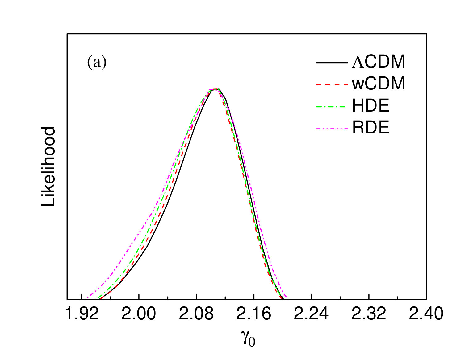 Figure 1
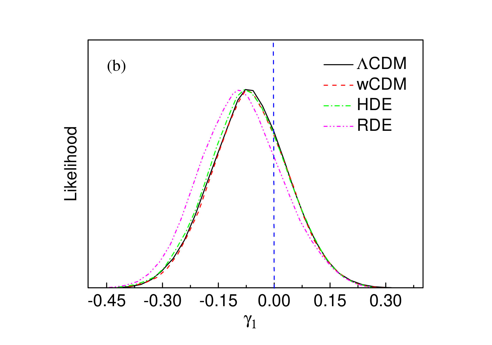 Figure 2
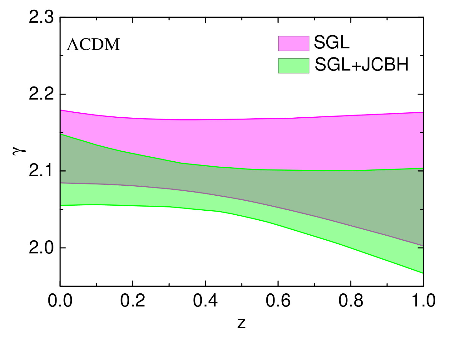 Figure 3
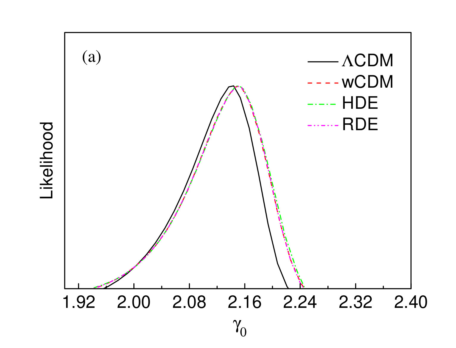 Figure 4
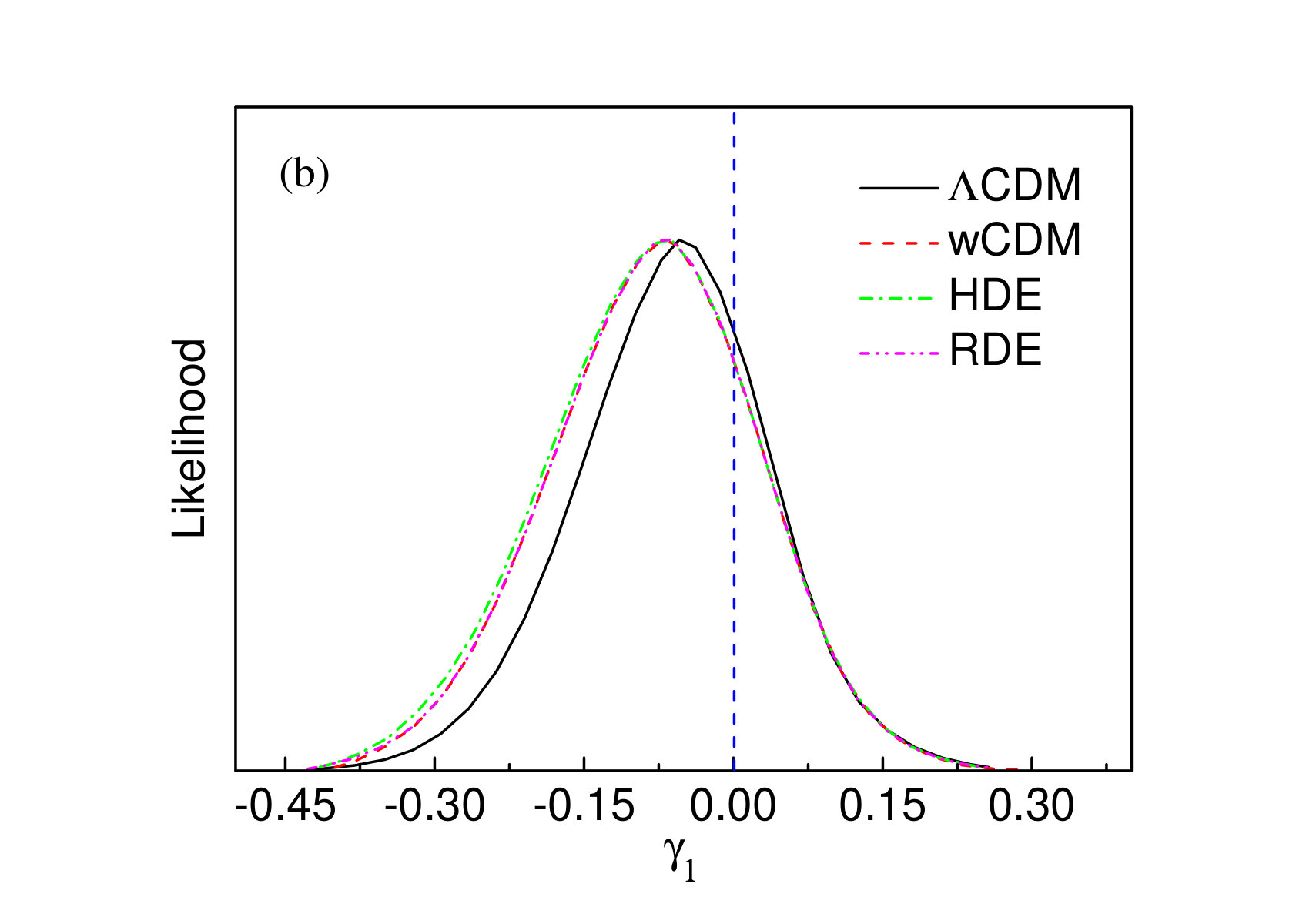 Figure 5
| Observation | ||||
|---|---|---|---|---|
| SGL | ||||
| SGL+JLA | ||||
| SGL+CMB | ||||
| SGL+BAO | ||||
| SGL+ | ||||
| SGL+JCBH |
| Model | CDM | HDE | RDE | ||||||
|---|---|---|---|---|---|---|---|---|---|
| Observation | SGL | SGL+JCBH | SGL | SGL+JCBH | SGL | SGL+JCBH | |||
| Model parameter | |||||||||
Peer Reviews
No public reviews on file for this paper yet. If you reviewed it on a platform where reviews are public (OpenReview, ICLR, NeurIPS, ICML), you can paste yours below so the community can read it here.
Videos
No videos yet. Explain this paper in a talk, walkthrough, or lecture? Add one.
No evidence for the evolution of mass density power-law index from strong gravitational lensing observation
Jing-Lei Cui
Department of Physics, College of Sciences, Northeastern University, Shenyang 110819, China
Hai-Li Li
Department of Physics, College of Sciences, Northeastern University, Shenyang 110819, China
Xin Zhang111Corresponding author
Department of Physics, College of Sciences, Northeastern University, Shenyang 110819, China
Center for High Energy Physics, Peking University, Beijing 100080, China
Abstract
In this paper, we consider the singular isothermal sphere lensing model that has a spherically symmetric power-law mass distribution . We investigate whether the mass density power-law index is cosmologically evolutionary by using the strong gravitational lensing (SGL) observation, in combination with other cosmological observations. We also check whether the constraint result of is affected by the cosmological model, by considering several simple dynamical dark energy models. We find that the constraint on is mainly decided by the SGL observation and independent of the cosmological model, and we find no evidence for the evolution of from the SGL observation.
strong gravitational lensing, mass density power-law index, dynamical dark energy, cosmological parameter estimation
pacs:
95.36.+x, 98.80.Es, 98.80.-k
Introduction
Strong gravitational lensing (SGL) observation has been largely developed in recent years and it has the potential to become an important astrophysical tool for probing both cosmology and galaxies. In an SGL system, the ratio of the proper angular diameter distances between lens and source and between observer and source can be measured. Since these distances depend on cosmological geometry, one can thus use the ratio to constrain cosmological models when adequate accurate SGL data can be obtained. For works on the issue concerning the SGL observation, see, e.g., Refs. [1, 2, 3, 4, 5, 6, 7, 8].
When calculating the ratio, mass distribution and evolution of the strong-lensing system based on lens model should be considered. Recently, it was shown in Ref. [9] that, when a spherically symmetric power-law total mass-density profile model, , is considered, a hint of the cosmological evolution of the power-law index (at around the level) can be found. This result is of great interest because the evolution of is important for the studies of galaxy structure. Thus, more recently, this issue was revisited in Refs. [10, 11]. In Ref. [10], the singular isothermal sphere (SIS) lens model is adopted and the power-law index is taken as a free parameter fitted together with cosmological parameters by using a reasonable sample of strong lenses. But, in this work, when estimating parameters, the present-day fractional energy density of matter is fixed at . Furthermore, in Ref. [11], in order to precisely constrain , the SGL observation is combined with the baryonic acoustic oscillations (BAO) and type Ia supernovae (SNIa) observations. In this study [11], the result of and is obtained based on the CDM model, for the parametrization , with the combination of SGL and BAO data, which implies that a time-varying power-law index is not supported.
The aim of the present paper is to carefully check whether the evidence of the cosmological evolution of can be found from the analysis of SGL observation (in combination with other various cosmological observations). We take two key steps to make the analysis: (i) we constrain the time-varying (parametrized in the form of ) in the CDM model by using the SGL data combined with different cosmological observations, and (ii) we further check if the constraint result is relevant to the cosmological model considered in the analysis. The current cosmological observations used in this work include: the SNIa data from the “joint light-curve analysis” (JLA) compilation, the cosmic microwave background (CMB) anisotropy data from the Planck 2015 observation, the BAO data from the 6dFGS, SDSS-DR7, and BOSS-DR11 surveys, and the Hubble parameter measurements (see Ref. [12] for a summary of the data). The typical dark energy models considered in this work include: the constant dark energy model (also abbreviated as the CDM model), the holographic dark energy (HDE) model [13], and the Ricci dark energy (RDE) model [14], all of which are the models with one more parameter than the CDM model.
This paper is organized as follows. In Section 2, we briefly describe the observational data. In Section 3, we constrain the time-varying in the CDM model by using the different combinations of SGL with other observations. In Section 4, we test the constraint results in dynamical dark energy models. Conclusion is given in Section 5.
Observational data
In this section, we briefly describe the observational data used in this work, including SGL, SNIa, CMB, BAO, and measurements. Throughout this paper, we consider a spatially flat Friedmann-Robertson-Walker (FRW) universe consisting of dark energy (de), matter (m) and radiation (r).
2.1 Strong gravitational lensing
In strong lensing system, light rays from a source to us can be bent when they pass a massive galaxy or galaxy cluster acting as lens, which forms multiple images of the source, arcs or Einstein rings. Mass distribution model within the lens is related to the parameters of lensing system directly or indirectly. In this paper, we consider the SIS model generalized to the spherically symmetric power-law mass distribution , following Ref. [10]. To make SGL probe usable in parameter estimation, the Einstein radius in an SIS lens must be used, which is expressed as
[TABLE]
where
[TABLE]
is the velocity dispersion inside an aperture with size , is the mass density power-law index, and are the proper angular diameter distances between lens and source and between observer and source, respectively. The proper angular diameter distance in a flat FRW universe is given by
[TABLE]
where is the dimensionless Hubble expansion rate, depending on the specific cosmological model, and km s*-1* Mpc*-1* is the Hubble constant ( is the reduced Hubble constant). To constrain cosmological models, we use the distance ratio
[TABLE]
The observable can be gained from Eq. (1). Accordingly, the uncertainty of is
[TABLE]
Here, it is assumed that the fractional uncertainty of the Einstein radius is at the level of , i.e., for all the lenses.
In the cosmological fit, we replace with the aperture-corrected velocity dispersion (, where is the effective radius). We use to make the observable more homogeneous for the sample of lenses located at different redshifts, and to make the fitting results more consistent with the previous analysis; see Ref. [10] for more details. Moreover, we consider mass density power-law index evolving with redshift, i.e., , where and are free parameters. We use data sample of strong lenses from Table of Ref. [10] compiled from the Sloan Lens ACS Survey (SLACS) [15, 16], BOSS emission-line lens survey (BELLS) [17], Lens Structure and Dynamics (LSD) [18, 19, 20], and Strong Lensing Legacy Survey (SL2S) [21, 22].
We fit the parameters by minimizing the following function,
[TABLE]
2.2 Type Ia supernova
We use the JLA compilation of spectroscopically confirmed SNIa with high quality light curves [23]. Theoretically, the relation of standardized distance modulus to luminosity distance for an SNIa is given by
[TABLE]
and
[TABLE]
where and denote the CMB frame and heliocentric redshifts, respectively. In the JLA analysis, the distance modulus of an SNIa is quantified by an empirical linear model,
[TABLE]
where is the observed peak magnitude in the rest frame B band, is the absolute magnitude, discribes the time stretching of the light curve, is the supernova color at maximum brightness. The two nuisance parameters and are assumed to be constants for all SNIa. For the JLA supernova, the function is
[TABLE]
where is the covariance matrix of , and can be found in Ref. [23].
2.3 Cosmic microwave background
We adopt the “Planck distance priors” from the Planck 2015 observation [24]. The distance priors include the shift parameter , the acoustic scale and the baryon density . They are respectively defined as
[TABLE]
[TABLE]
and
[TABLE]
where is the present-day fractional energy density of baryon, is the proper angular diameter distance at the redshift of the decoupling epoch of photon , and is the comoving sound horizon at the photon-decoupling epoch. Here, is given by
[TABLE]
where with and being the present-day baryon and photon energy densities, respectively, , and . is given by the fitting formula [25],
[TABLE]
where
[TABLE]
We use the mean values and covariance matrix of for the Planck TT+LowP data from Ref. [24]. The function for CMB is
[TABLE]
where , , and .
2.4 Baryon acoustic oscillations
Through BAO measurements, one can get the ratio of the effective distance measure and the comoving sound horizon . The spherical average gives us the expression of ,
[TABLE]
The comoving sound horizon size can be calculated by using Eq. (14), where denotes the redshift of the drag epoch, whose fitting formula is given by [26],
[TABLE]
where
[TABLE]
We use four BAO data points from the 6dF Galaxy Survey [27], the SDSS-DR7 [28] and the BOSS-DR11 [29] surveys. The function for BAO is
[TABLE]
The concrete information of corresponding to the four BAO data points is explicitly given in Ref. [30] (see also Refs. [31, 32]).
2.5 Hubble parameter
Measuring directly the Hubble parameter is very important for exploring the history of cosmic evolution. Reference [12] sorted out data from the measurements of clustering of galaxies or quasars [29, 33, 34, 35] and differential age [36, 37, 38, 39]. In Table 1 of Ref. [12], the data of versus the redshift and corresponding errors are listed. The function for is
[TABLE]
where .
Constraining time-varying in the CDM model
In this section, we constrain the time-varying , in the form of , along with other cosmological parameters, in the CDM model, by using the different combinations of SGL with other cosmological observations.
For the CDM model, the dimensionless Hubble expansion rate is expressed as
[TABLE]
where we have the fractional density of radiation and the effective number of neutrino species .
In this analysis, we consider the cases of SGL alone, SGL+JLA, SGL+CMB, SGL+BAO, SGL+, and SGL+JCBH. Here, for convenience, we use the abbreviation JCBH to denote the combination of JLA+CMB+BAO+. The constraint results of , , , and are summarized in Table 1. From the table, we find that the constraint results of all the data combinations are consistent with each other (except for that the SGL alone cannot precisely constrain and ). In all the cases, we find that (with the uncertainty around 0.04–0.05) and (with the uncertainty around 0.1), which indicates that the time-varying is not favored by the current observations.
We find that the SGL data alone can constrain tightly, and when other cosmological observations are considered, the constraint results are not affected greatly. This indicates that is indeed an astrophysical parameter, without cosmological evolution. For all the cases, the result is consistent with at round the 0.6 level. In Fig. 1, we reconstruct the evolution according to the constraint results of the cases SGL alone and SGL+JCBH. From the figure, we clearly see that the two cases are well consistent with each other, both in good agreement with a constant (with ).
From Table 1, we can clearly see that using the SGL data alone cannot strictly constrain and . When the SGL observation is combined with JCBH, the results of and are consistent with those from Planck ( and ) [40]. In the case of SGL+JCBH, we obtain and , which is the fit result of from the current cosmological observations.
Constraints in dynamical dark energy models
In this section, we check if the constraint result of derived in the last section is affected by the cosmological model. Thus, we consider several dynamical dark energy models to make a test. We only consider the simplest models, i.e., the CDM model, the HDE model, and the RDE model, all of which have only one more parameter than CDM.
For the CDM model, we have constant, and thus is written as
[TABLE]
For the HDE model, the density of dark energy is defined by [13]
[TABLE]
where is a dimensionless parameter, is the reduced Planck mass defined by , and is the infrared (IR) cutoff, given by the future event horizon of the universe,
[TABLE]
with the scale factor of the universe. The cosmological evolution of this model is governed by the following differential equations:
[TABLE]
and
[TABLE]
where is the fractional density of dark energy and . For extensive studies on the HDE model, see, e.g., Refs. [41, 42, 43, 44, 45, 46, 47, 48, 49, 50, 51, 52].
For the RDE model, the density of dark energy is also given by Eq. (25). The different point is that the IR cutoff is related to the Ricci scalar curvature, [14, 53, 54, 55, 56, 57, 58]. Accordingly, in this model, dark energy density is defined as [14]
[TABLE]
where is a positive constant. Then we can get
[TABLE]
The constraint results for the CDM, HDE, and RDE models are listed in Table 2. From Table 2, we find that the best-fitting and as well as their corresponding errors for the three models are almost the same to each other when the SGL data only is used. Furthermore, by comparing Table 2 with Table 1, we can see that the results of and are also very similar to those of the CDM model. We plot the 1D marginalized probability distributions of and for the CDM, CDM, HDE, and RDE models in Fig. 2. We can clearly see that the curves of the dynamical dark energy models are almost degenerate and their deviation from the result of the CDM model is also very small.
When the combination of SGL and JCBH is used in parameter estimation, we find that the changes for the fit results of and , compared to the case of SGL alone, are very small. In this case, the 1D marginalized probability distributions of and for the CDM, CDM, HDE and RDE models are plotted in Fig. 3. We also find that the curves are very close to each other. From Table 2, we find that using SGL data alone cannot tightly constrain the cosmological parameters, such as and , and model parameters (, , and ). To constrain these parameters well, the SGL data must be combined with other cosmological observations. Our analysis shows that the cosmological model doest not affect the constraint result of .
Conclusion
In this paper, we wish to clarify whether the mass density power-law index is cosmologically evolutionary by using the SGL observation, in combination with other cosmological observations. We constrain the time-varying , in the form of , in the CDM model, with the data combinations SGL alone, SGL+JLA, SGL+CMB, SGL+BAO, SGL+, and SGL+JCBH. We find that the constraint results of all the data combinations are consistent with each other, and in all the cases we derive (with the uncertainty around 0.04–0.05) and (with the uncertainty around 0.1), which indicates that the time-varying is not supported by the current observations. Our result is consistent with at round the 0.6 level. We then check whether the constraint result of is affected by the cosmological model, by considering the CDM, HDE, and RDE models. We find that the constraint result of is not relevant to the cosmological model. Therefore, we conclude that there is no evidence for the cosmological evolution of from the current SGL observation.
Acknowledgements
This work was supported by the National Natural Science Foundation of China (Grants No. 11522540 and No. 11690021), the Top-Notch Young Talents Program of China, and the Provincial Department of Education of Liaoning (Grant No. L2012087).
The reference list from the paper itself. Each links out to its DOI / PubMed record.
- 1[1] Z. H. Zhu, Mod. Phys. Lett. A 15 (2000) 1023 [astro-ph/0010351].
- 2[2] K. H. Chae, G. Chen, B. Ratra and D. W. Lee, Astrophys. J. 607 (2004) L 71 [astro-ph/0403256].
- 3[3] Z. H. Zhu and M. Sereno, Astron. Astrophys. 487 (2008) 831 [ar Xiv:0804.2917 [astro-ph]].
- 4[4] S. Cao, Y. Pan, M. Biesiada, W. Godlowski and Z. H. Zhu, JCAP 1203 (2012) 016 [ar Xiv:1105.6226 [astro-ph.CO]].
- 5[5] K. Liao and Z. H. Zhu, Phys. Lett. B 714 (2012) 1 [ar Xiv:1207.2552 [astro-ph.CO]].
- 6[6] J. Wu, Z. Li, P. Wu and H. Yu, Sci. China Phys. Mech. Astron. 57 (2014) 988.
- 7[7] Y. Chen, C. Q. Geng, S. Cao, Y. M. Huang and Z. H. Zhu, JCAP 1502 (2015) 02, 010 [ar Xiv:1312.1443 [astro-ph.CO]].
- 8[8] J. Cui, Y. Xu, J. Zhang and X. Zhang, Sci. China Phys. Mech. Astron. 58 , 110402 (2015) [ar Xiv:1511.06956 [astro-ph.CO]].