A survey on Morse boundaries & stability
Matthew Cordes

TL;DR
This survey reviews the current state of research on Morse boundaries and stability, summarizing key results and developments in the field.
Contribution
It compiles and discusses known results on Morse boundaries and stability, providing a comprehensive overview of the topic.
Findings
Summarizes key results in Morse boundaries
Highlights recent advances in stability theory
Identifies open problems and future directions
Abstract
In this paper we survey many of the known results about Morse boundaries and stability.
Click any figure to enlarge with its caption.
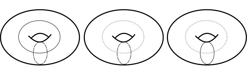 Figure 1
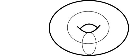 Figure 2
Peer Reviews
No public reviews on file for this paper yet. If you reviewed it on a platform where reviews are public (OpenReview, ICLR, NeurIPS, ICML), you can paste yours below so the community can read it here.
Videos
No videos yet. Explain this paper in a talk, walkthrough, or lecture? Add one.
Taxonomy
TopicsMathematical Dynamics and Fractals
A survey on Morse boundaries & stability
Matthew Cordes
1 generalizing hyperbolicity
Recently there have been efforts to generalize tools used in the setting of Gromov hyperbolic spaces to larger classes of spaces. We survey here two aspects of these efforts: Morse boundaries and stable subspaces. Both the Morse boundary and stable subspaces are systematic approaches to collect and study the hyperbolic aspects of finitely generated groups. We will see in this survey a nice relationship between the two approaches.
Throughout the survey we will expect the reader to be familiar with the basics of geometric group theory. For details on this material see [bridson:1999fj] and for additional information especially on boundaries of not-necessarily-geodesic hyperbolic spaces see [Buyalo:2007ab].
We begin with an important definition that has its roots in a classical paper of Morse [morse:1924aa]:
Definition 1.1**.**
A geodesic in a metric space is called -Morse if there exists a function such that for any -quasi-geodesic with endpoints on , we have , the -neighborhood of . We call the function a Morse gauge. A geodesic is Morse if it is -Morse for some .
In a geodesic -hyperbolic space, the Morse lemma says there is a Morse gauge which depends only on such that every ray is -Morse, i.e., the behavior of quasi-geodesics (on a large scale) is similar to that of geodesics. This property fails in a space like . On the other hand, if every geodesic in some geodesic space is -Morse, then the space is -hyperbolic, where depends on .
There are a few other competing definitions of geodesics which admit “hyperbolic like” properties: geodesics which satisfy a contracting property, geodesics with superlinear divergence, and having cut points in the asymptotic cone. (See Section 2.1 for the definition of the contracting property and [charney:2015aa, Arzhantseva:2016aa, drutu:2005aa] for the others.) All of these notions have been used extensively to analyze many groups and spaces: right-angled Artin groups [behrstock:2012aa, koberda:2014aa, cordes:2016aa], Teichmüller space [minsky:1996aa, Behrstock:2006aa, Sultan:2014aa, Brock:2006aa, Brock:2011aa], the mapping class group and curve complex [Masur:1999aa, Masur:2000aa, durham:2015aa, bestvina:2015ab], spaces [Behrstock:2014aa, Sultan:2014aa], [Algom-Kfir:2011aa], relatively hyperbolic groups and spaces [drutu:2005aa, Osin:2006aa], acylindrically hyperbolic groups [dahmani:2011aa, sisto:2016aa, bestvina:2015ab], and small cancellation groups [Arzhantseva:2016ab] among others. Furthermore these properties find applications in rigidity theorems such as Mostow Rigidity in rank-1 [Paulin:1996aa] and the Rank Rigidity Conjecture for spaces [Ballmann:1995aa, Bestvina:2009aa, Caprace:2010aa].
Geodesics of these types all have a relationship to the Morse property. In [charney:2015aa] Charney and Sultan show that Morse, superlinear ‘lower divergence’, and ‘strongly’ contracting are equivalent notions in spaces. In [Arzhantseva:2016aa] the authors characterize Morse quasi-geodesics in arbitrary geodesic metric spaces and show they are ‘sublinearly’ contracting and have ‘completely superlinear’ divergence. In [drutu:2010aa] the authors show that a quasi-geodesic is Morse if and only if it is a cut point in every asymptotic cone. This plays a key role in showing that metric relative hyperbolicity is preserved by quasi-isometry [drutu:2005aa].
While groups may have no Morse geodesics, Sisto in [sisto:2016aa] shows that every acylindrically hyperbolic group has a bi-infinite Morse geodesic. This class of groups, recently unified by Osin in [osin:2016aa], encompasses many groups of significant interest in geometric group theory: hyperbolic and relatively hyperbolic groups, non-directly decomposable right-angled Artin groups, mapping class groups, and . There are groups outside this class which contain Morse geodesics. Examples of these groups appear in [olcprimeshanskii:2009aa]; these groups have been shown to have infinitely many Morse geodesics but are not acylindrically hyperbolic. At the other extreme, any groups which admit a law do not contain any Morse geodesics [drutu:2005aa]. It is easy to see that for has no Morse geodesics: take any geodesic ray and consider a right angled isosceles triangle whose hypotenuse is on . It is easy to check that the other two edges form a -quasi-geodesic with endpoints on . This is true no matter how large the triangle and thus these uniform quasi-geodesics can be arbitrarily far from and therefore violate the Morse condition.
In this survey we will overview the notion of Morse boundaries with increasing generality in Sections 2 and 3. In Section 3 we will also introduce stability, the notion of stable equivalence, two ‘stable equivalence’ invariants and end with some calculations of these invariants. In Section 4 we will spend some time discussing stable subgroups and introduce a boundary characterization of convex cocompactness which is equivalent to stability. Finally, in Section 5 we will discuss a topology on the contracting boundary which is second countable and thus metrizable.
2 contracting and Morse boundaries
Boundaries have been an extremely fruitful tool in the study of hyperbolic groups. The visual boundary, as a set, is made up of equivalence classes of geodesic rays, where one ray is equivalent to the other if they fellow travel. Roughly, one topologizes the boundary by declaring open neighborhoods of a ray to be the rays that stay close to for a long time. Gromov showed that a quasi-isometry between hyperbolic metric spaces and induces a homeomorphism on the visual boundaries. In the setting of a finitely generated group acting geometrically on and , then the quasi-isometry from to induced by these actions extends -equivariantly to a homeomorphism of their boundaries. This means, in particular, that the boundary of a hyperbolic group (as a topological space) is independent of the choice of (finite) generating set.
The boundary of a hyperbolic group is a powerful tool to study the structure of the group. For instance, Bowditch and Swarup relate topological properties of the boundary to the JSJ decomposition of a hyperbolic group [Bowditch:1998aa, Swarup:1996aa]. Bestvina and Mess in [Bestvina:1991aa] relate the virtual cohomological dimension of a hyperbolic group to the dimension of the boundary of . Boundaries have also been instrumental in the proofs of quasi-isometric rigidity theorems, particularly Mostow Rigidity in rank 1 [Paulin:1996aa].
There is also a robust boundary theory of relatively hyperbolic groups using the Bowditch boundary introduced in a 1998 preprint of Bowditch that was recently published [Bowditch:2012aa]. Bowditch used this boundary to analyze JSJ decompositions [Bowditch:1998aa, Bowditch:2001aa]. Groff showed that if a group is hyperbolic relative to a collection of subgroups which are not properly relatively hyperbolic, then the Bowditch boundary is a quasi-isometry invariant [Groff:2013aa].
The topology on the visual boundary for a space can be defined in a manner similar to the visual boundary of a hyperbolic space. Hruska and Kleiner show that in the case of a space with isolated flats, this boundary is a quasi-isometry invariant [Hruska:2005aa]. Unfortunately, Croke and Kleiner produced an example of a right-angled Artin group which acts geometrically on two quasi-isometric spaces which have non-homeomorphic visual boundaries [Croke:2000aa], hence the boundary of a group is not well-defined. More surprising is that Wilson shows that this group admits an uncountable collection of distinct boundaries [Wilson:2005aa]. Charney and Sultan in [charney:2013qy] showed that if one restricts attention to rays with hyperbolic-like behavior, contracting rays, then one can construct a quasi-isometry invariant boundary for any complete space. They call this boundary the contracting boundary.
2.1 contracting boundaries
We begin with a description of the contracting boundary of a space introduced in [charney:2015aa]. We will start with some explication on contracting geodesics.
Definition 2.1** (contracting geodesics).**
Given a fixed constant , a geodesic is said to be -contracting if for all ,
[TABLE]
where is the closest point projection to . We say that is contracting if it is -contracting for some . An equivalent definition is that any metric ball not intersecting projects to a segment of length on .
Remark 2.2**.**
This definition is sometimes referred to as strongly contracting. To see a more general definition of contracting and its relationship with the Morse property and divergence see Section 5 and for more details [Arzhantseva:2016aa]. This more general definition is used by Cashen to answer a question of Charney–Sultan (see Theorem 2.11) and by Cashen–Mackay to construct a topology on the contracting boundary that is metrizable (see Section 5).
It is easy to see that any geodesic in a flat will not be contracting because the projection of any ball onto a geodesic will just be the diameter of the ball. In a hyperbolic space all geodesics are uniformly contracting. Contracting geodesics appear in many groups and spaces, for instance: psuedo-Anosov axes in Teichmüller space [minsky:1996aa], iwip axes in the Outer Space of outer automorphisms of a free group [Algom-Kfir:2011aa], and axes of rank 1 isometries of spaces [Ballmann:1995aa, Bestvina:2009aa].
Remark 2.3** (Morse and (strongly) contracting are not equivalent).**
If is proper geodesic space, then contracting implies Morse [Algom-Kfir:2011aa]. In this generality the converse is not true. Consider a ray and a set of intervals of length on . To the endpoints of these intervals attach an edge of length . Let be the resulting space. The ray is not contracting because balls can have unbounded projection onto . To see that is Morse, we need to check to check that there exits an constant so that for any -quasi-geodesic with endpoints on , . By [bridson:1999fj, III.H Lemma 1.11] we can replace with a ‘tame’ quasi-geodesic with three nice properties: and have the same endpoints, and have Hausdorff distance less than , and the length between any two points on of is bounded by a linear function of the (with constants depending only on ). Since the length of the attached intervals is while the distance between their endpoints is , in order for to cross such a segment, we must have is less than a linear function of . Thus must only cross finitely many of the attached segments. Thus for for any -quasi-geodesic with endpoints on we can choose that where is the length of the longest attached interval travels over.
In the setting of spaces Sultan shows that Morse and contracting are equivalent notions [Sultan:2014aa] and in [charney:2015aa] Charney and Sultan reprove this fact with explicit control on the constants. Charney and Sultan also characterize contracting geodesics in cube complexes using a combinatorial criterion which gives an effective tool for analyzing the boundary. We will use this characterization to help us compute Examples 2.6 and 2.8.
Let be a space. We define the visual boundary, , to be the set of equivalence classes of geodesic rays up to asymptotic equivalence and denote the equivalence class of a ray by . It is an elementary fact that, for a complete space and a fixed basepoint, every equivalence class can be represented by a unique geodesic ray emanating from . One natural topology on is the cone topology. We define the topology of the boundary with a system of neighborhood bases. A neighborhood basis for is given by open sets of the form:
[TABLE]
That is, two geodesic rays in the cone topology are close if they fellow travel (at distance less than ) for a long time (at least time ). This topology is independent of choice of basepoint. When we refer to the visual boundary we will always assume that means with the cone topology unless otherwise stated.
Let be a complete space with basepoint . We define the contracting boundary of a space to be the subset of the visual boundary consisting of all contracting geodesics:
[TABLE]
In order to topologize the contracting boundary we consider a collection of increasing subsets of the boundary,
[TABLE]
one for each . We topologize each with the subspace topology from the visual boundary of . We note that there is an obvious continous inclusion map for all . We can topologize the whole boundary by taking the direct limit over these subspaces. Thus with the direct limit topology. Recall that this means a set is open (resp. closed) in if and only if is open (resp. closed) for all .
One nice property of this boundary is that if we fix a contracting constant , then is compact and behaves very much like the boundary of a hyperbolic space, an analogy we will build on in Section 3.
Another nice property is that the direct limit topology on does not depend on the choice of basepoint so we will freely denote the contracting boundary as without mention of basepoint.
2.1.1 examples
We will focus on examples for the contracting boundary for a couple reasons. First, other more general incarnations of the Morse boundary, which we will see later, are homeomorphic to the contracting boundary in the case of a space. Second, there is a combinatorial characterization of contracting geodesics in cube complexes (see [charney:2015aa, Theorem 4.2]) that makes the computations more transparent.
Example 2.4** (, hyperbolic spaces).**
Revisiting the conversation of which spaces have contracting geodesics, when for or more generally the product of two unbounded space will have no contracting geodesics because any geodesic will be contained in a flat. This means that will be empty. On the other hand, if is and hyperbolic, then will be the Gromov boundary because every ray will uniformly contracting. For example, will be homeomorphic to .
Example 2.5** (hyperbolic with a dash of flat).**
Now consider the space formed by gluing a Euclidean half-plane to a bi-infinite geodesic in the hyperbolic plane . Picking to be our basepoint, we see that any geodesic in the half-plane (including ) will not be Morse, but all the other rays in will still be contracting. So the boundary will be the union of two open intervals. We can already see here how the contracting boundary differs from the Gromov boundary, because it is not necessarily compact. In fact, Murray shows that the contracting boundary of a space is compact if any only if is hyperbolic [murray:2015aa].
Example 2.6** ().**
For a slightly more complicated example consider the space formed by the wedge product of a loop and a torus and its fundamental group . See Figure 1. The universal cover of , , is a cube complex [Charney:1995aa]. Consider a geodesic ray in . It is not hard to see that the contracting constant of only depends on how long subsegments of spend in the cosets of the subgroup (because of the tree-graded structure of ), and it is only contracting if there is a uniform bound on the length of these subsegments. In fact, the contracting constant is half that uniform bound; thus each is the set of geodesic rays which have subsegments of lenght at most in the cosets with the subspace topology. So is the direct limit over these spaces. Later we will see in Theorem 3.17 that the subspace of formed by the union of all -contracting geodesics with basepoint is quasi-isometric to a proper simplicial tree and thus has boundary homeomorphic to a Cantor set.
Remark 2.7** (the contracting boundary is not in general first-countable).**
The topology of the contracting boundary is in general quite fine relative to the subspace topology. In fact, in [murray:2015aa] Murray shows that the space as defined above is not first-countable (and thus not metrizable). We present Murray’s argument here: We choose the basepoint of to be some lift of the wedge point in . We first note that the geodesic ray is [math]-contracting. We define a collection of geodesic rays . Note that the each of the are -contracting and not -contracting for any . If we fix a , it is clear that that the converge to in the contracting boundary. Consider a new sequence where is any function . We note that the intersection of with is finite for each and thus closed in the subspace topology and therefore in . Ergo, the cannot converge to in the contracting boundary.
A general fact for all first-countable spaces is that if you have a countable collection of sequences which all converge to the same point, it is always possible to pick a ‘diagonal’ sequence which also converges to that point. That is, if were first-countable, since converges to for fixed , then there would be a function so that converges to . As we saw above, this cannot happen. Since all metric spaces are first countable, this means that the contracting boundary is not, in general, metrizable! In fact, Murray, in the same paper, shows if is a space with a geometric action, then is metrizable if any only if is hyperbolic.
Example 2.8** (Croke–Kleiner).**
Recall that Croke and Kleiner produced an example of a right-angled Artin group that acts geometrically on two quasi-isometric spaces which have non-homeomorphic visual boundaries [Croke:2000aa]. Their example is a right-angled Artin group
[TABLE]
The Salvetti complex of this group, , is three tori with the middle torus glued to the other two along orthogonal curves corresponding to the generators and . See Figure 2. As in the example above, it follows from [Charney:1995aa] that the universal cover of , , is a cube complex.
Let be the union of the -torus and the -torus in and its inverse image in . Each component of the inverse image decomposes as the direct product of the Cayley graph of the free group on two elements and . Thus the contracting boundary of each component of is empty. The same fact holds for , the union of the -torus and the -torus in . Croke and Kleiner refer to the components as “blocks”. As in the example above, it follows that in order for a geodesic ray in to be contracting, there must be a uniform bound on the length of the subsegments of which intersect the blocks. The converse of this holds by the combinatorial characterization by Charney and Sultan of contracting geodesics in cube complexes [charney:2015aa]. Thus, is contracting if and only if there is a uniform bound on the length of subsegments of which intersect a single block. We will revisit this in Example 2.10 after we describe some of the properties of the contracting boundary.
2.1.2 properties of the boundary
This boundary has many desirable properties. First and foremost it is a quasi-isometry invariant. That is, if and are two complete spaces and is a quasi-isometry, then induces a homeomorphism . Furthermore since each is compact, the boundary is -compact. Finally it is a visibility space. In summary:
Theorem 2.9** ([charney:2015aa]).**
Given a complete space , the contracting boundary, , equipped with the direct limit topology, is
- (1)
independent of choice of basepoint; 2. (2)
-compact, i.e., the union of countably many compact sets; 3. (3)
a visibility space, i.e., any two points in the contracting boundary can be joined by a bi-infinite contracting geodesic; and 4. (4)
a quasi-isometry invariant.
Example 2.10** (Croke–Kleiner redux).**
Croke and Kleiner produce the two spaces on which acts geometrically by modifying the metric on in a very simple way: they skew the angles between the and curves making the -cubes parallelograms. This is enough to change the homeomorphism type of the visual boundary. In fact, Wilson shows that any two distinct angles between the and curves produces non-homeomorphic boundaries [Wilson:2005aa]. Qing showed that if you keep the angles and change the side lengths of the cubes then the identity map does not induce a homeomorphism on the boundary [Qing:2013aa].
In the examples of Croke–Kleiner and Wilson, the parts of the boundary which change the homeomorphism type are the parts that come from the intersection of the blocks. These points do not appear in the contracting boundary. Neither do the points in the Qing example. The parts of the boundary which change are the rays which stay longer and longer time in successive blocks. These examples suggest that the restriction to contracting rays may be optimal if you want a quasi-isometry invariant.
In [charney:2015aa], Charney and Sultan remarked that a quasi-isometry induces a bijection on the contracting rays and the set of contracting rays could be topologized with just the subspace topology from the visual boundary. They asked if a quasi-isometry would induce a homeomorphism on the boundary with this topology. In [Cashen:2016aa] Cashen answers this question in the negative:
Theorem 2.11** ([Cashen:2016aa]).**
In general a quasi-isometry will not induce a homeomorphism on the contracting boundary with the subspace topology.
Cashen’s examples, though, are pathological in nature and open questions still remain: If are spaces with cocompact isometry groups and if is a quasi-isometry, does induce a homeomorphism on the contracting boundary with the subspace topology? Are these two boundaries abstractly homeomorphic?
One can also ask when a homeomorphism between the boundaries of two spaces is induced by a quasi-isometry. In the case of a hyperbolic spaces, Paulin [Paulin:1996aa] gives conditions under which this holds. Recent work of Charney and Murray [Charney:2017aa] gives some analogous conditions for the contracting boundaries of cocompact CAT(0) spaces.
2.1.3 dynamics on the contracting boundary
In the realm of hyperbolic groups there is a classical notion of North-South dynamics:
Theorem 2.12**.**
If is a hyperbolic group acting geometrically on a proper geodesic metric space and if is an infinite order element, then for all open sets and with and there exists an so that .
It is well known that the classical notion of North-South dynamics of axial isometries on the visual boundary of a space fails because there are isometries which fix whole flats. Rank-1 isometries, though, do act on the visual boundary with North-South dynamics [Ballmann:1995ab, Hamenstadt:2009aa]. Since rank-1 isometries of spaces are contracting, one might hope that North-South dynamics hold on the contracting boundary. This is not the case. Again we will present an example from [murray:2015aa].
Example 2.13** (Example 2.6 revisited).**
Again, we consider and the spaces and . Let be an axis for . Let be the geodesic defined by the word . Again we note that the do not converge to in the contracting boundary because is finite for every and thus is closed in . We note that the set is an open set around but for all we have for all .
In [murray:2015aa] Murray does prove a weaker type of North-South dynamics on the contracting boundary.
Theorem 2.14** (Corollary 4.3 [murray:2015aa]).**
Let be a proper space and let be a group acting geometrically on . If is a rank-1 isometry in , i.e., a contracting element, is an open neighborhood of and is a compact set in then for sufficiently large , .
Murray also uses dynamical methods to prove a classical result that is known for the action of a hyperbolic group on its boundary.
Theorem 2.15** (Theorem 4.1 [murray:2015aa]).**
Let be a group acting geometrically on a proper space. Either is virtually or the orbit of every point in the contracting boundary is dense.
In Section 2.2 we will introduce a generalization of the contracting boundary to any proper geodesic space. It is unknown if any of these dynamical results hold in the more general settings.
2.2 Morse boundary
The Morse boundary, introduced by Cordes in [cordes:2016ad], generalizes the contracting boundary to the setting of proper geodesic spaces. This boundary retains many of the nice properties of the contracting boundary including quasi-isometry invariance and visibility. In the case of a proper space it is the contracting boundary, and in the case of a proper hyperbolic space it is the Gromov boundary. The generality in which this boundary is defined means it is a quasi-isometry invariant for every finitely generated group.
We will see later in Section 3 that there is a more general definition of the Morse boundary of a not-necessarily-proper geodesic space. This definition will use the Gromov product and will carry more structure, but it is often helpful to reduce to the case when the boundary can be defined by geodesics instead of sequences (as we will see in Section 4.1) for proper geodesic spaces.
Let be a proper geodesic space and fix a basepoint . The Morse boundary of , , is the set of all Morse geodesic rays in (with basepoint ) up to asymptotic equivalence. To topologize the boundary, first fix a Morse gauge and consider the subset of the Morse boundary that consists of all rays in with Morse gauge at most :
[TABLE]
Unlike in the case of a space, the visual topology of the boundary of a proper geodesic may not even be well-defined. So, instead, we take a page from the definition of the Gromov topology on the boundary of a hyperbolic space. This first step is a lemma in [cordes:2016ad] that says that two -Morse geodesic rays with the same basepoint which fellow travel stay uniformly close and that uniform bound, , only depends on . Thus we can topologize this set in a similar manner as one does for the Gromov boundary of hyperbolic spaces: the topology is defined by a system of neighborhoods, , at a point in . The sets are defined to be the set of geodesic rays with basepoint and for all . That is, two -Morse rays are close in if they stay closer than for a long time.
Let be the set of all Morse gauges. We put a partial ordering on so that for two Morse gauges , we say if and only if for all . We define the Morse boundary of to be
[TABLE]
with the induced direct limit topology, i.e., a set is open in if and only if is open for all .
The Morse boundary retains almost all of the properties of the contracting boundary. The one exception is that it is open whether or not the Morse boundary is -compact because a priori the direct limit is over an uncountable set.
Theorem 2.16** ([cordes:2016ad]).**
Given a proper geodesic space , the Morse boundary, , equipped with the direct limit topology, is
- (1)
a visibility space, i.e., any two points in the Morse boundary can be joined by a bi-infinite Morse geodesic; 2. (2)
independent of choice of basepoint; 3. (3)
a quasi-isometry invariant; and 4. (4)
homeomorphic to the Gromov boundary if is hyperbolic and to the contracting boundary if is .
One useful property of the Morse boundary is that compact subsets consist of uniformly Morse geodesics [murray:2015aa, cordes:2016ab]. Futhermore, as in the case of the contracting boundary, a group has a compact Morse boundary if any only if it is hyperbolic [cordes:2016ab].
3 (metric) Morse boundary and stability
An alternative approach to understanding “hyperbolic directions” in a metric space is to understand “hyperbolic” or quasi-convex subgroups/subspaces. In the case of hyperbolic groups, quasi-convex subgroups are finitely generated and undistorted. Furthermore these properties are preserved under quasi-isometry. In a general group, though, quasi-convexity depends on a choice of generating set and is not preserved by quasi-isometry. Thus in an effort to preserve these qualities, we look at a stronger notion of quasi-convexity:
Definition 3.1**.**
We say a quasi-convex subspace of a geodesic metric space is -stable if every pair of points in can be connected by a geodesic which is -Morse in . We say that a subgroup is stable if it is stable as a subspace.
Remark 3.2** (Relationship with Durham–Taylor definition).**
It is important to note that this is a generalization of the original definition of stability given by Durham–Taylor in [durham:2015aa]. The definition above detects the same collection of stable subsets up to quasi-isometry, and the two definitions coincide for subgroups of finitely generated groups [cordes:2016aa, Lemma 3.8].
Durham–Taylor prove that the collection of stable subgroups of mapping class groups are precisely those which are convex-cocompact in the sense of Farb–Mosher [farb:2002aa, durham:2015aa]. These subgroups are well studied and have important connections to the geometry of Teichmüller space, the curve complex and surface group extensions. In the setting of right-angled Artin groups, Koberda, Manghas, and Taylor classify all the stable subgroups. They prove that these subgroups are all free [koberda:2014aa]. For more on the history and current situation of stable subgroups see Section 4.
We will see in this section that the notions of the Morse boundary and of stability can be united. We will do this by viewing any geodesic metric space as the union of stable subsets which are indexed by Morse gauges and hyperbolic (with hyperbolicity constant depending only on ). We will define these subspaces in Section 3.2, but before this we will recall some definitions.
3.1 sequential boundary, capacity dimension & asymptotic dimension
Definition 3.3**.**
Let be a metric space and let . The Gromov product of and with respect to is defined as
[TABLE]
Let be a sequence in . We say converges at infinity if as . Two convergent sequences are said to be equivalent if as . We denote the equivalence class of by .
The sequential boundary of , denoted , is defined to be the set of convergent sequences considered up to equivalence.
Definition 3.4** (4-point definition of hyperbolicity; Definition [bridson:1999fj]).**
Let be a (not necessarily geodesic) metric space. We say is –hyperbolic if for all we have
[TABLE]
If is –hyperbolic, we may extend the Gromov product to in the following way:
[TABLE]
where and the supremum is taken over all sequences and in such that and .
Recall that a metric on is said to be visual (with parameter ) if there exist such that , for all .
Let . As a shorthand we define .
Theorem 3.5**.**
[Ghys:1990aa, Section ]* Let be a –hyperbolic space. If then we can construct a visual metric on such that*
[TABLE]
Visual metrics on a hyperbolic space are all quasi-symmetric. A quasi-symmetry is a map that is a generalization of bi-Lipschitz map: instead of controlling how much the diameter of a set can change, a quasi-symmetry preserves only the relative sizes of sets.
Definition 3.6**.**
A homeomorphism is said to be quasi–symmetric if there exists a homeomorphism such that for all distinct ,
[TABLE]
One natural quasi-isometry invariant assigned the boundary of a hyperbolic space is the capacity dimension. This invariant was introduced by Buyalo in [Buyalo:2005aa] and it is sometimes known as linearly-controlled dimension.
Let be an open covering of a metric space . Given , we let
[TABLE]
be the *Lebesgue number of at * and the Lebesgue number of . The multiplicity of , , is the maximal number of members of with non-empty intersection.
Definition 3.7** ([Buyalo:2007ab]).**
The capacity dimension of a metric space , , is the minimal integer with the following property:
There exists some such that for every sufficiently small there is an open covering of by sets of diameter at most with and .
The capacity dimension is similar to the covering dimension in that it is an infimum over open covers, but the capacity dimension necessitates metric information: given an open cover the capacity dimension requires a linear relationship between the and . For more information see [Buyalo:2007ab].
In [Buyalo:2005aa, Corollary 4.2], Buyalo shows that the capacity dimension of a metric space is a quasi-symmetry invariant and since quasi-isometries of hyperbolic spaces induce quasi-symmetries on the boundaries, this shows that the capacity dimension of the boundary is an invariant of a hyperbolic space.
Another quasi-isometry invariant dimension one can assign to a metric space is the asymptotic dimension. This notion was introduced by Gromov in [gromov:1993aa] and is a coarse version of the topological dimension.
Definition 3.8**.**
A metric space has asymptotic dimension at most (), if for every there exists a cover of by uniformly bounded sets such that every metric –ball in intersects at most elements of the cover. We say has asymptotic dimension if but .
The celebrated theorem of Yu showed that groups with finite asymptotic dimension satisfy both the coarse Baum–Connes and the Novikov conjectures [yu:1998aa]. Many classes of groups have been shown to have finite asymptotic dimension including: hyperbolic groups [Roe:2005aa], relatively hyperbolic groups whose parabolic subgroups are of finite dimension [osin:2005aa], mapping class groups [bestvina:2015ab], cubulated groups [wright:2012aa]. But exact bounds are often hard to calculate.
Buyalo and Lebedeva used the capacity dimension to prove a conjecture of Gromov: the asymptotic dimension of any hyperbolic group is the topological dimension of its boundary plus one [Buyalo:2007aa].
3.2 stable strata
Definition 3.9** (stable stratum).**
Let be a geodesic metric space and . We define to be the set of all points in which can be joined to by an -Morse geodesic.
What do these stable strata look like? First, we can easily see that given there exists such that by choosing . So the collection of will cover . If is hyperbolic, since all geodesics are -Morse for some , we have that for that . On the other hand, if is a space with no infinite Morse geodesics (e.g., groups satisfying non-trivial laws or products of unbounded spaces) then the are just sets of bounded diameter. For groups with mixed geometries this is a hard question to answer. We will see later in the survey (Sections 3.4 and 3.5) that (up to quasi-isometry) we can begin to understand these subspaces for some groups.
One thing we do know is that these subspaces are hyperbolic. A standard argument shows that if then the geodesic triangle in formed by is -slim [cordes:2016ad, Lemma 2.2] proving these spaces are hyperbolic. Note, though, that the geodesic is not necessarily contained in . So since the are not necessarily geodesic, we use the 4-point definition of hyperbolicity and conclude they are hyperbolic.
Using the fact that these triangles are slim, one can also show that if then is -Morse where depends only on [cordes:2016ad, Lemma 2.3]. This shows that the are not only quasi-convex, but they are -stable!
Furthermore, as each is hyperbolic we may consider its Gromov boundary, , and the associated visual metric . (See [Buyalo:2007ab, Section 2.2] for a careful treatment of the sequential boundary of a hyperbolic space which is not necessarily geodesic.) This metric is unique up to quasi-symmetry.
Natural maps between strata have nice properties: the natural inclusion induces a map which is a quasi-symmetry onto its image. Additionally, if we have a quasi-isometry , then for every there exists an such that . This induces an embedding which is a quasi-symmetry onto its image. We will see in Section 3.3 that these properties will be useful in defining new quasi-isometry invariants.
Finally, if is also a proper metric space, then for each there is a homeomorphism between (as defined in Section 2.2 with geodesics) and and thus the Morse boundary is homeomorphic to direct limit over as topological spaces.
In summary:
Theorem 3.10** ([cordes:2016aa]).**
Let be geodesic metric spaces and let . The family of subsets of indexed by functions enjoys the following properties:
- I
(covering) . 2. II
(partial order) If , then . 3. III
(hyperbolicity) Each is hyperbolic in the sense of Definition 3.4. 4. IV
(stability) Each is -stable, where depends only on . 5. V
(universality) Every stable subset of is a quasi-convex subset of some . 6. VI
(boundary) The sequential boundary can be equipped with a visual metric which is unique up to quasi-symmetry. An inclusion induces a map which is a quasi-symmetry onto its image. 7. VII
(generalizing the Gromov boundary) If is hyperbolic, then for all sufficiently large, and is quasi-symmetric to the Gromov boundary of . 8. VIII
(generalizing the Morse boundary) If is proper, then its Morse boundary is equal to the direct limit of the as topological spaces. 9. IX
(behavior under quasi-isometry) If is a quasi-isometry then for every there exists an such that and there is an induced embedding which is a quasi-symmetry onto its image.
There is a stronger version of 3.10.IX, but we will first we require some additional terminology.
Let be geodesic metric spaces, let and . We say is stably subsumed by (denoted ) if, for every there exists some and a quasi-isometric embedding . By 3.10.IX, this property is independent of the choice of . We say and are stably equivalent (denoted ) if they stably subsume each other. It is easy to see that two spaces are stably equivalent if and only if they have the same collection of stable subsets up to quasi-isometry.
Given a geodesic metric space , we will consider the collection of boundaries equipped with visual metrics as the metric Morse boundary of .
We say that one collection of spaces is quasi-symmetrically subsumed by another (denoted ) if, for every there exists a and an embedding which is a quasi–symmetry onto its image. Two collections are quasi-symmetrically equivalent (denoted ) if and ).
Theorem 3.10.IX’.
Let be geodesic metric spaces, let and . Then if and only if .
Corollary 3.11**.**
Quasi-isometric geodesic metric spaces are stably equivalent and have quasi-symmetrically equivalent metric Morse boundaries. In particular, the metric Morse boundary is invariant under change of basepoint.
Stable equivalence is a much weaker notion than quasi-isometry. All spaces with no infinite Morse geodesic rays will be stably equivalent to a point! On the other hand, Cordes–Hume show that the mapping class group and Teichmüller space with the Teichmüller metric are stably equivalent (Theorem 3.16), when it is well known that they are not quasi-isometric.
3.3 stable equivalence invariants
We can now define two stable equivalence invariants using the notions discussed in Section 3.1; in particular, the capacity dimension and the asymptotic dimension. The definitions will rely on Theorem 3.10.
Definition 3.12** (stable asymptotic dimension).**
The stable asymptotic dimension of () is the supremal asymptotic dimension of a stable subset of
We can see that by universality it is possible to just consider the maximal asymptotic dimension of the . One obvious but useful bound is that the stable asymptotic dimension is bounded from above by the asymptotic dimension.
Definition 3.13** (Morse capacity dimension).**
The Morse capacity dimension of () is the supremal capacity dimension of spaces in the metric Morse boundary. We say that the empty set has capacity dimension .
By Theorem 3.10.VI we know that the inclusion map induces a map which is a quasi-symmetry onto its image. So this definition is well defined.
It follows from Theorem 3.10 that these notions are invariant under change of basepoint and a stable equivalence invariant and thus a quasi-isometry invariant. It also follows that the stable dimension of a hyperbolic space is precisely its asymptotic dimension and the Morse capacity dimension of a hyperbolic space is the capacity dimension of its boundary equipped with some visual metric.
Remark 3.14** (conformal dimension).**
Since the conformal dimension (introduced by Pansu in [Pansu:1989aa]) is also a quasi-symmetry invariant, one could also define a conformal dimension of the Morse boundary in the same manner and with the properties listed above, but it is often harder to compute.
By using bounds bounds proved in the hyperbolic setting, we get a nice relationship between these two dimensions [Buyalo:2005aa, Theorem ], [Mackay:2013aa, Proposition ].
Proposition 3.15**.**
Let be a geodesic metric space. Then
[TABLE]
3.4 calculations in finitely generated groups
We now present some calculations in finitely generated groups where Morse geodesics have been characterized in some way: mapping class groups, right-angled Artin groups, and graphical small cancellation groups. As we will see, a recurring way to calculate an upper bound on the stable asymptotic dimension is to show that each stable stratum embeds into a hyperbolic space that is easier to understand.
3.4.1 mapping class group and Teichmüller space
Assume that is an orientable surface of finite type. Let be the Teichmüller space of with the Teichmüller metric. The following result is a generalization of a result in [cordes:2016ad] which shows that is homeomorphic to .
Theorem 3.16** ([cordes:2016aa]).**
* and are stably equivalent thus . Furthermore and are bounded above linearly in the complexity of .*
An upper bound on the stable asymptotic dimension of mapping class groups can be obtained via the bounds on the asymptotic dimension for mapping class groups obtained by Bestvina–Bromberg–Fujiwara in [bestvina:2015ab] or by Behrstock–Hagen–Sisto in [behrstock:2015aa] which are exponential or quadratic in the complexity of the surface respectively. To show there is a linear bound on the stable asymptotic dimension, Cordes–Hume show each stable subset of quasi-isometrically embeds into the curve graph. They then use the bound found by Bestvina–Bromberg on the asymptotic dimension of the curve graph [bestvina:2015aa].
Leininger and Schleimer prove that for every there is a surface such that the Teichmüller space contains a stable subset quasi–isometric to [leininger:2014aa]. This fact gives a lower bound on the stable dimension, which is at best logarithmic in the complexity, but also shows that Teichmüller spaces can have arbitrarily high stable asymptotic dimension. Since is stably equivalent to , we see that contains a stable subset quasi-isometric to . The only known explicit examples of convex cocompact subgroups of mapping class groups are virtually free groups [Dowdall:2014ab, Kent:2009aa, koberda:2014aa, Min:2011aa]. Although the results of Leininger–Schleimer do not provide any non-virtually-free convex cocompact subgroups, the fact that for some surfaces shows that there is no purely geometric obstruction to the existence of a non-free convex cocompact subgroup of .
3.4.2 right-angled Artin groups
Koberda, Manghas, and Taylor classify the stable subgroups of all right-angled Artin groups [koberda:2014aa]. They show that these subgroups are always free. The next theorem is the natural analogue for stable subspaces.
Theorem 3.17** ([cordes:2016aa]).**
Let be a Cayley graph of a right–angled Artin group. Every stable subset of is quasi-isometric to a proper tree. In particular, is stably equivalent to a line if the group is Abelian of rank , a point if it is Abelian of rank and a regular trivalent tree otherwise.
The proof of this theorem follows in a very similar manner to the proof of Theorem 3.16. In this case each stable subset of embeds into the contact graph (defined by Hagen [hagen:2014aa]), which is a quasi-tree. As a result, each is quasi-isometric to a proper tree. The proof is completed by calling on the universality condition in Theorem 3.10. By universality of stable subsets (Theorem 3.10.V), we know that any stable subgroup of a right-angled Artin group is quasi-isometric to a proper simplicial tree. Thus since groups which are quasi-isometric to trees are virtually free [Ghys:1990aa, Corollary 7.19], they recover a result of [koberda:2014aa]: stable subgroups of right–angled Artin groups are free.
3.4.3 graphical small cancellation
We move to the realm of graphical small cancellation groups. Graphical small cancellation theory is a generalization introduced by Gromov [gromov:2003aa] in order to construct groups whose Cayley graphs contain certain prescribed subgraphs, in particular one can construct “Gromov monster” groups, those with a Cayley graph which coarsely contains expanders [Arzhantseva:2008aa, Osajda:2014aa]. These monster groups cannot be coarsely embedded into a Hilbert space, and they are the only known counterexamples to the Baum–Connes conjecture with coefficients [Higson:2002aa].
Theorem 3.18** ([cordes:2016aa]).**
Let be the Cayley graph of a graphical small cancellation group. Then and .
Note that this is optimal as fundamental groups of higher genus surfaces are hyperbolic with asymptotic dimension and admit graphical small cancellation presentations.
Again, we work with the stable strata. Each of the strata embeds quasi-isometrically into a finitely presented classical small cancellation group. These groups are hyperbolic with asymptotic dimension at most and the capacity dimension of their Gromov boundaries is at most .
3.5 relatively hyperbolic groups
Osin in [osin:2005aa] shows that relatively hyperbolic groups inherit finite asymptotic dimension from their maximal parabolic subgroups. This is also true for the stable asymptotic dimension:
Theorem 3.19** ([cordes:2016aa]).**
Let be a finitely generated group which is hyperbolic relative to . Then if and only if for all .
In [cordes:2016ac] Cordes–Hume focus on relatively hyperbolic groups. In this paper they suggest an approach to answering the following question which appears in [Behrstock:2009aa]: How may we distinguish non-quasi-isometric relatively hyperbolic groups with non-relatively hyperbolic peripheral subgroups when their peripheral subgroups are quasi-isometric?
Using small cancellation theory over free products Cordes–Hume construct quasi-isometrically distinct one-ended relatively hyperbolic groups which are all hyperbolic relative to the same collection of groups. These groups are distinguished using a notion similar to stable asymptotic dimension; rather than , we use stable subsets which “avoid” the left cosets of the peripheral subgroups.
Theorem 3.20** ([cordes:2016ac]).**
Let be a finite collection of finitely generated groups each of which has finite stable dimension or are non-relatively hyperbolic. There is an infinite family of -ended groups , which are non-quasi-isometric, where each is hyperbolic relative to .
4 stable subgroups
We will start our discourse on stable subgroups with some with some motivation from Kleinian groups and mapping class groups.
A non-elementary discrete (Kleinian) subgroup determines a minimal -invariant closed subspace of the Riemann sphere called its limit set and taking the convex hull of determines a convex subspace of with a -action. A Kleinian group is called convex cocompact if it acts cocompactly on this convex hull or, equivalently, any -orbit in is quasiconvex.
Originally defined by Farb–Mosher [farb:2002aa] and later developed further by Kent–Leininger [Kent:2008aa] and Hamenstädt [Hamenstadt:2005aa], a subgroup is called convex cocompact if and only if any -orbit in , the Teichmüller space of with the Teichmüller metric, is quasiconvex, or acts cocompactly on the weak hull of its limit set in the Thurston compactification of . This notion is important because convex cocompact subgroups are precisely those which determine Gromov hyperbolic surface group extensions. Furthermore, Farb–Mosher show that if there is a purely pseudo-Anosov subgroup of that is not convex cocompact, then this subgroups would be a counterexample to Gromov’s conjecture that every group with a finite Eilenberg–Mac Lane space and no Baumslag–Solitar subgroups is hyperbolic (see [Kent:2007aa] for more information).
In both of these examples, convex cocompactness is characterized equivalently by both a quasi-convexity condition and an asymptotic boundary condition. In [durham:2015aa], Durham–Taylor introduced stability in order to characterize convex cocompactness in by a quasiconvexity condition intrinsic to the geometry of and this condition naturally generalizes the above quasi-convexity characterizations of convex cocompactness to any finitely generated group. There has been much recent work to characterize stable subgroups of important groups. The theorem below is a brief summary of this work.
Theorem 4.1**.**
Let the pair of a finitely generated group and a subgroup satisfy one of the following:
- (1)
* is hyperbolic and is quasi-convex;* 2. (2)
G is relatively hyperbolic and is a finitely generated and quasi-isometrically embeds in the the coned off graph in the sense of [Farb:1998aa]; 3. (3)
* is a right-angled Artin group with a finite graph which is not a join and is a finitely generated subgroup quasi-isometrically embedded in the extension graph [koberda:2014aa];* 4. (4)
* and is a convex cocompact subgroup in the sense of [farb:2002aa];* 5. (5)
* and is a convex cocompact subgroup in the sense of [Hamenstadt:2014aa];* 6. (6)
* is hyperbolic and hyperbolically embedded in ;*
Then is stable in . Moreover for (1), (3), and (4), the reverse implication holds.
Item (1) follows easily by checking the definition. Item (2) is due to [Aougab:2016aa], for (3) this is due to [koberda:2014aa], for (4) this is due to [durham:2015aa], for (5) this is again [Aougab:2016aa], and for (6) this follows from [sisto:2016aa].
4.1 boundary cocompactness
There is an alternative characterization to the Durham–Taylor notion of stability using the Morse boundary to define an asymptotic property for subgroups of finitely generated groups called boundary convex cocompactness which generalizes the classical boundary characterization of convex cocompactness from Kleinian groups. This is presented in [cordes:2016ab].
Let be a finitely generated group acting by isometries on a proper geodesic metric space . Fix a basepoint . In order to define this boundary characterization we first need to define a limit set.
Definition 4.2** ().**
The limit set of the -action on is
[TABLE]
That is, the limit set is the set of points which can be represented by sequences of uniformly Morse -orbit points; note that is obviously -invariant. It is also invariant under change of basepoint.
Given some we know there is a sequence so that . We can produce a geodesic from this sequence in a standard way: for each let be an -Morse geodesic joining and . It follows from Arzelà–Ascoli that there is a subsequence which converges (uniformly on compact sets) to a geodesic ray that is -Morse by [cordes:2016ad, Lemma 2.8]. This map defines a homeomorphism between the Morse boundary defined by sequences and the Morse boundary defined by geodesics [cordes:2016aa, Theorem 3.14]. From this perspective, by Theorem 2.16 we know that there exists a bi-infinite Morse geodesic joining any two distinct points in the limit set. This is a starting point for defining the weak hull, but we want to define it by taking all geodesics with distinct endpoints in . Formalizing this motivates the next definition:
Definition 4.3** (asymptotic, bi-asymptotic).**
Let be a biinfinite geodesic in with a closest point to along . Let . We say is forward asymptotic to if for any -Morse geodesic ray with , there exists such that
[TABLE]
We define backwards asymptotic similarly. If is forwards, backwards asymptotic to , respectively, then we say is bi-asymptotic to .
Now for the definition of weak hull.
Definition 4.4** (weak hull).**
The weak hull of in based at , denoted , is the collection of all biinfinite rays which are bi-asymptotic to for some .
An important fact about the weak hull is that of , then is nonempty and -invariant.
We are now ready to define boundary convex cocompactness:
Definition 4.5** (boundary convex cocompactness).**
We say that acts boundary convex cocompactly on if the following conditions hold:
- (1)
acts properly on ; 2. (2)
For some (any) , is nonempty and compact; 3. (3)
For some (any) , the action of on is cobounded.
Definition 4.6** (Boundary convex cocompactness for subgroups).**
Let be a finitely generated group. We say is boundary convex cocompact if acts boundary convex cocompactly on any Cayley graph of with respect to a finite generating set.
Theorem 4.7** ([cordes:2016ab]).**
Let be a finitely generated group. Then is boundary convex cocompact if and only if is stable in .
Theorem 4.7 is an immediate consequence of the following stronger statement:
Theorem 4.8** ([cordes:2016ab]).**
Let be a finitely generated group acting by isometries on a proper geodesic metric space . Then the action of is boundary convex cocompact if and only if some (any) orbit of in is a stable embedding.
In both cases, is hyperbolic and any orbit map extends continuously and -equivariantly to an embedding of which is a homeomorphism onto its image .
We note that Theorem 4.7 and [durham:2015aa, Proposition 3.2] imply that boundary convex cocompactness is invariant under quasi-isometric embeddings.
Remark 4.9** (The compactness assumption on is essential for Theorem 4.8).**
Consider the group acting on its Cayley graph. Consider the subgroup . Since the is isometrically embedded and convex in , it follows that and for any , whereas is not hyperbolic and thus not stable in . In fact, the compactness assumption ensures that the weak hull will be a subspace of some , i.e., hyperbolic.
The following is an interesting question:
Question 4.10**.**
If , then must we have in fact ?
Recall from Section 2.1.3 that in the case of spaces, this question has been affirmatively answered [murray:2015aa, Lemma 4.9].
4.1.1 height, width, bounded packing
Antolín, Mj, Sisto and Taylor in [Antolin:2016aa] use the boundary cocompactness characterization to extend some well-known intersection properties of quasi-convex subgroups of hyperbolic or relatively hyperbolic groups [Gitik:1998aa, Hruska:2009aa] to the context of stable subgroups of finitely generated groups:
Theorem 4.11**.**
Let be stable subgroups of a finitely generated group. Then the collection satisfies the following:
- (1)
H has finite height. 2. (2)
H has finite width. 3. (3)
H has bounded packing.
In particular they show any group-subgroup pair satisfying one of the conditions in Theorem 4.1 then has finite height, finite width, and bounded packing.
5 a metrizable topology on the Morse boundary
Cashen and Mackay have introduced a topology on the Morse boundary of a proper geodesic space that is metrizable [Cashen:2017aa]. They use a generalized notion of contracting geodesics which follows that of Arzhantseva, Cashen, Gruber, and Hume [Arzhantseva:2016aa]. We present the definition here:
Definition 5.1**.**
We call a function sublinear if it is non-decreasing, eventually non-negative, and .
Definition 5.2**.**
Let be a proper geodesic metric space. Let be a geodesic ray, and let be the closest point projection to . Then, for a sublinear function , we say that is -contracting if for all and in :
[TABLE]
We see that Definition 2.1 is simply this definition if we ask that is the constant function . We revisit the example in Remark 2.3: the space was a ray with set of intervals of length with an interval of length attached to the endpoints of . We noted that this ray was not strongly contracting. It is not hard to see that in this more general definition, that it is -contracting. We showed in Remark 2.3 that this ray was Morse. This fact is no coincidence; in proper geodesic spaces -contracting is equivalent to being Morse [Arzhantseva:2016aa].
Cashen and Mackay introduce a new topology on the contracting boundary that is finer than the “subspace topology” defined with the Gromov product but less fine than the direct limit topology. They call this topology the topology of fellow-traveling quasi-geodesics and denote it . The idea is that a geodesic is close to a geodesic if all quasi-geodesics tending to closely fellow-travel quasi-geodesics tending to for a long time.
One major difference from the direct limit topology on the Morse boundary is that rays with increasingly bad contracting functions can converge to a contracting ray. Recall again the space from Example 2.6 and the collection of rays from Remark 2.7 . Consider the sequence . It is not hard to see that this converges in the topology of the fellow-traveling quasi-geodesics to the geodesic ray . The set will be compact in . We note that the ray has a constant contracting function , so this compact set has arbitrarily bad contracting geodesics.
The topology keeps many of the desirable properties of the Morse boundary with the direct limit topology. First they show that it is a quasi-isometry invariant. Second, they also show that this boundary is second countable, and thus metrizable. Finally, they prove a weak version of North-South dynamics for the action of a group on its contracting boundary in à la Theorem 2.14 by Murray. Third, they show that if you restrict the topology to rays which live in a single stratum and take the direct limit then this is homeomorphic to the Morse boundary. Finally they show that if is hyperbolic then this boundary is homeomorphic to the Gromov boundary. In summary:
Theorem 5.3** ([Cashen:2017aa]).**
Let be a proper geodesic space. The contracting boundary with the topology, , is
- (1)
a quasi-isometry invariant; 2. (2)
second countable and thus metrizable; 3. (3)
* is homeomorphic to the Morse boundary;* 4. (4)
homeomorphic to the Gromov boundary if is hyperbolic; 5. (5)
has weak North-South dynamics à la Theorem 2.14.
There are still many open questions about this topology: It is know that this topology is not in general homeomorphic to the subspace topology, but the example given is not a space with a geometric groups action. Is this topology different from the subspace topology in the presence of a geometric group action? We know the space is metrizable, but can we give a useful description of a metric? If so can we show that if is a quasi-isometry then a quasi-symmetry?
References