Oxygen budget in low-mass protostars: the NGC1333-IRAS4A R1 shock observed in [OI] at 63 um with SOFIA-GREAT
L.E. Kristensen, A. Gusdorf, J.C. Mottram, A. Karska, R. Visser, H., Wiesemeyer, R. G\"usten, R. Simon

TL;DR
This study investigates the oxygen content in a low-mass protostar outflow, finding that about 15% of oxygen is atomic and associated with the outflow, challenging previous assumptions about water being the main oxygen reservoir.
Contribution
First spectrally resolved detection of [OI] 63 um line in a protostellar outflow, quantifying atomic oxygen presence and its relation to other molecules in the shock region.
Findings
Approximately 15% of oxygen is atomic in the outflow shock.
CO is the dominant oxygen carrier with an abundance of ~10^-4.
A significant portion of [OI] emission originates from the outflow
Abstract
In molecular outflows from forming low-mass protostars, most oxygen is expected to be locked up in water. However, Herschel observations have shown that typically an order of magnitude or more of the oxygen is still unaccounted for. To test if the oxygen is instead in atomic form, SOFIA-GREAT observed the R1 position of the bright molecular outflow from NGC1333-IRAS4A. The [OI] 63 um line is detected and spectrally resolved. From an intensity peak at +15 km/s, the intensity decreases until +50 km/s. The profile is similar to that of high-velocity (HV) H2O and CO 16-15, the latter observed simultaneously with [OI]. A radiative transfer analysis suggests that ~15% of the oxygen is in atomic form toward this shock position. The CO abundance is inferred to be ~10^-4 by a similar analysis, suggesting that this is the dominant oxygen carrier in the HV component. These results demonstrate that…
Click any figure to enlarge with its caption.
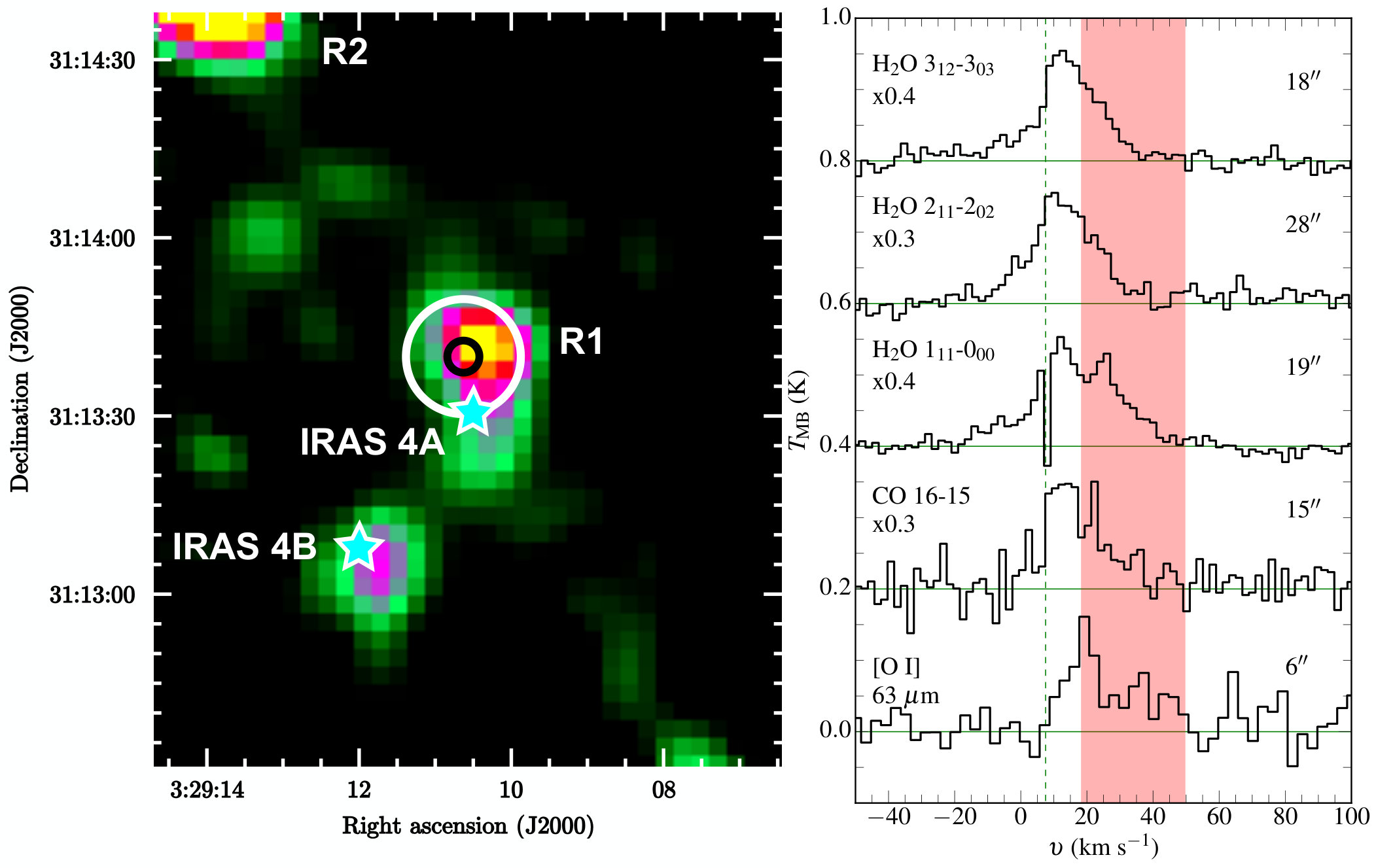 Figure 1
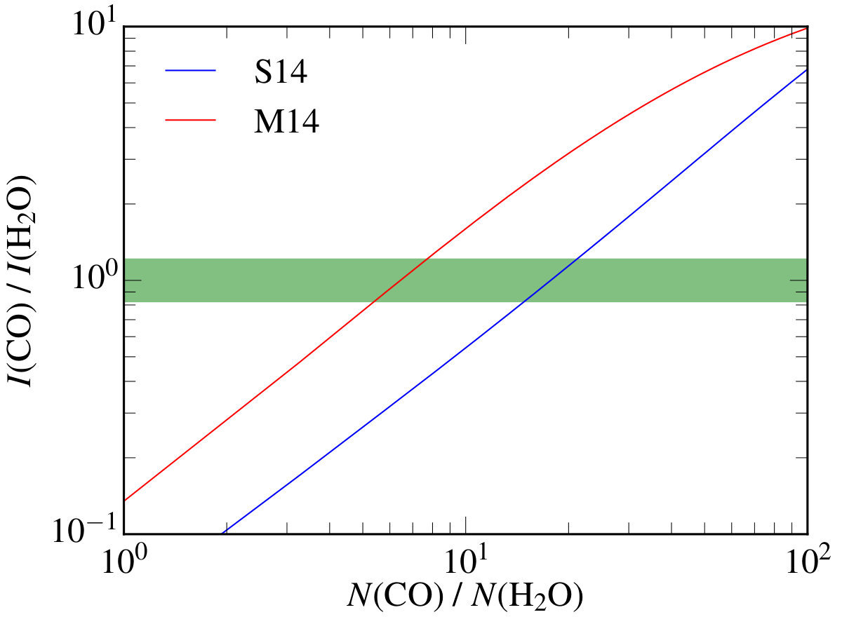 Figure 2
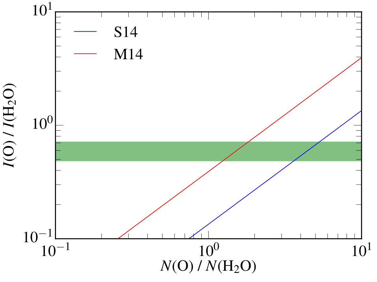 Figure 3
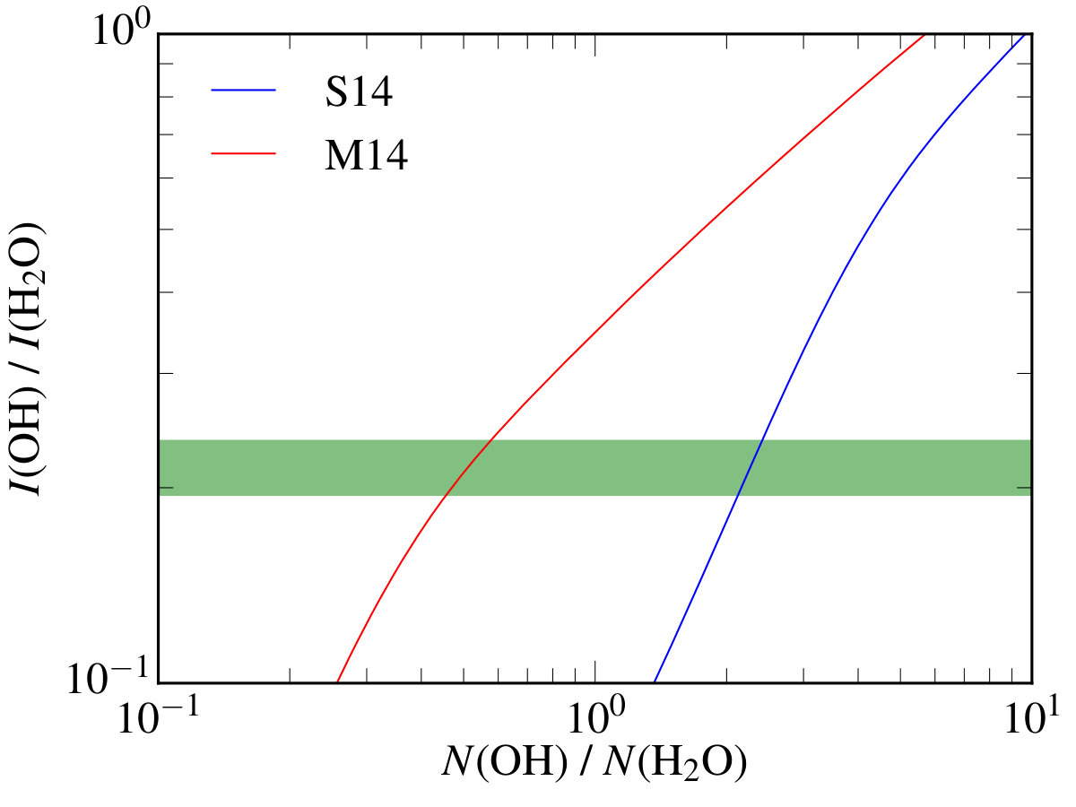 Figure 4
| Line | rmsa𝑎aa𝑎aIn 2 km s-1 channels. | d | PACS |
|---|---|---|---|
| (mK) | (K km s-1) | (K km s-1) | |
| [O i] 63m | 33 | 2.7 | 1.0 |
| CO 16–15 | 77 | 11 | 9 |
| OH(1834 GHz) | 52 | 1.0b𝑏bb𝑏b3 limit for a width of 20 km s-1. | 1.2 |
| Line ratio | Obs. | M14a𝑎aa𝑎aAverage spot shock conditions, Mottram et al. (2014). | B14b𝑏bb𝑏bL1157-B1, Busquet et al. (2014). | S12c𝑐cc𝑐cL1448-R4 HV emission, Santangelo et al. (2012). | S14d𝑑dd𝑑dNGC1333-IRAS4A R2, Santangelo et al. (2014). |
|---|---|---|---|---|---|
| 110–101 / 111–000 | 0.73 | 0.75 | 1.32 | 1.18 | 0.79 |
| 211–202 / 111–000 | 1.00 | 0.56 | 0.98 | 0.25 | 0.68 |
| 312–303 / 111–000 | 0.60 | 0.50 | 0.16 | 0.13 | 0.26 |
| Least-squares | 0.20 | 0.54 | 0.99 | 0.22 |
| Parameter | M14a𝑎aa𝑎aSpot shock model results from Mottram et al. (2014). | S14b𝑏bb𝑏bNGC1333-IRAS4A R2 model results from Santangelo et al. (2014). |
|---|---|---|
| (K) | 750 | 1000 |
| (H2) (cm-3) | 3105 | 2105 |
| (AU)c𝑐cc𝑐cFor a source distance of 235 pc (Hirota et al. 2008). | 55 | 350 |
| (H2O) (cm-2) | 1.01017 | 1.01016 |
| (O) (cm-2) | 1.51017 | 4.21016 |
| (CO) (cm-2) | 6.31017 | 1.71017 |
| (OH) (cm-2)d𝑑dd𝑑d3 upper limit. | 5.01016 | 2.21016 |
| (O)e𝑒ee𝑒eAbundances are calculated as ()/(Otot) = (Y)/[(O)+(CO)+(H2O)], where (Otot)=310-4 is the abundance of volatile O w.r.t. H2. Including the (OH) upper limits will not significantly change relative abundances. | 5.010-5 | 5.710-5 |
| (H2O)e𝑒ee𝑒eAbundances are calculated as ()/(Otot) = (Y)/[(O)+(CO)+(H2O)], where (Otot)=310-4 is the abundance of volatile O w.r.t. H2. Including the (OH) upper limits will not significantly change relative abundances. | 3.510-5 | 1.410-5 |
| (CO)e𝑒ee𝑒eAbundances are calculated as ()/(Otot) = (Y)/[(O)+(CO)+(H2O)], where (Otot)=310-4 is the abundance of volatile O w.r.t. H2. Including the (OH) upper limits will not significantly change relative abundances. | 2.210-4 | 2.310-4 |
| C/O | 0.7 | 0.8 |
| Species | Transition | Freq. | a𝑎aa𝑎a = 10B. | Instr. | Beam | |
|---|---|---|---|---|---|---|
| (GHz) | (K) | (s-1) | (′′) | |||
| O | 3P1–3P2 | 4744.777 | 228 | 8.91(–5) | GREAT | 6.1 |
| CO | 16–15 | 1841.346 | 750 | 4.05(–4) | GREAT | 15.3 |
| OH | = –, –, – – + | 1834.760 | 270 | 6.45(–2) | GREAT | 15.3 |
| H2O | 110–101 | 556.936 | 61 | 3.46(–3) | HIFI | 38.1 |
| 111–000 | 1113.343 | 53 | 1.84(–2) | HIFI | 19.0 | |
| 211–202 | 752.033 | 137 | 7.06(–3) | HIFI | 29.2 | |
| 312–303 | 1097.365 | 249 | 1.65(–2) | HIFI | 19.3 |
| Line | Flux (10-16 W m-2) |
|---|---|
| [O i] 63m | 2.360.09 |
| [O i] 145m | 0.110.01 |
| CO 16–15 | 1.430.02 |
| OH(1838 GHz) | 0.100.02 |
| OH(1834 GHz) | 0.200.02 |
Peer Reviews
No public reviews on file for this paper yet. If you reviewed it on a platform where reviews are public (OpenReview, ICLR, NeurIPS, ICML), you can paste yours below so the community can read it here.
Videos
No videos yet. Explain this paper in a talk, walkthrough, or lecture? Add one.
11institutetext: Centre for Star and Planet Formation, Niels Bohr Institute and Natural History Museum of Denmark, University of Copenhagen, Øster Voldgade 5-7, DK-1350 Copenhagen K, Denmark, 11email: [email protected] 22institutetext: LERMA, Observatoire de Paris, École normale supérieure, PSL Research University, CNRS, Sorbonne Universités, UPMC Univ. Paris 06, F-75231, Paris, France 33institutetext: Max Planck Institute for Astronomy, Königstuhl 17, 69117 Heidelberg, Germany 44institutetext: Centre for Astronomy, Nicolaus Copernicus University, Faculty of Physics, Astronomy and Informatics, Grudziadzka 5, PL-87100 Torun, Poland 55institutetext: European Southern Observatory, Karl-Schwarzschild-Strasse 2, 85748 Garching, Germany 66institutetext: Max-Planck-Institute for Radioastronomy, Auf dem Hügel 69, 53121 Bonn, Germany 77institutetext: I. Physikalisches Institut der Universität zu Köln, Zülpicher Strasse 77, 50937 Köln, Germany
Oxygen budget in low-mass protostars: the NGC1333-IRAS4A R1 shock observed in [O i] at 63 m with SOFIA-GREAT
L.E. Kristensen 11
A. Gusdorf 22
J.C. Mottram 33
A. Karska 44
R. Visser 55
H. Wiesemeyer 66
R. Güsten 66
R. Simon 77
(Submitted: ; Accepted: )
In molecular outflows from forming low-mass protostars, most oxygen is expected to be locked up in water. However, Herschel observations have shown that typically an order of magnitude or more of the oxygen is still unaccounted for. To test if the oxygen is instead in atomic form, SOFIA-GREAT observed the R1 position of the bright molecular outflow from NGC1333-IRAS4A. The [O i] 63 m line is detected and spectrally resolved. From an intensity peak at +15 km s*-1* , the intensity decreases until +50 km s*-1*. The profile is similar to that of high-velocity (HV) H2O and CO 16–15, the latter observed simultaneously with [O i]. A radiative transfer analysis suggests that 15% of the oxygen is in atomic form toward this shock position. The CO abundance is inferred to be 10*-4* by a similar analysis, suggesting that this is the dominant oxygen carrier in the HV component. These results demonstrate that a large portion of the observed [O i] emission is part of the outflow. Further observations are required to verify whether this is a general trend.
Key Words.:
Stars: formation — ISM: molecules — ISM: jets and outflows — ISM: individual sources: NGC1333-IRAS4A-R1
1 Introduction
Oxygen is the third most abundant element in the Universe after hydrogen and helium. In the past few years, Herschel-PACS observations have confirmed that the [O i] 63m line emission is one of the dominant gas cooling lines at far-infrared (FIR) wavelengths, along with CO and H2O (e.g., Karska et al. 2013; 2014, Nisini et al. 2015). However, with a spectral resolution of 90 km s*-1*, it is unclear where the [O i] emission originates, even when considering velocity centroids (Dionatos & Güdel 2016). Only a handful of spectra show high-velocity line wings, indicating that only a small fraction of emission originates at \varv$$>100 km s*-1* (Nisini et al. 2015). The [O i] line profile at lower velocities may be complex (e.g., Leurini et al. 2015), and it is clear that [O i] emission does not follow more traditional outflow tracers such as low- CO emission (Mottram et al. 2017).
Two other major reservoirs of oxygen exist in protostellar outflows: CO and H2O (OH is not believed to be a major reservoir, Wampfler et al. 2013). CO is an abundant and chemically stable molecule, and it is typically assumed that all volatile carbon is locked up in this molecule for a total abundance of 10*-4* (Yıldız et al. 2013), an assumption that holds for some protostellar outflows where both CO and H2 are observed (Dionatos et al. 2013). The H2O abundance, on the other hand, is more uncertain and has proved difficult to determine. Observations with Herschel-HIFI suggest that the H2O abundance is 10*-7*–10*-5* toward outflow positions (e.g., Tafalla et al. 2013, Santangelo et al. 2014, Kristensen et al. 2017), which is orders of magnitude lower than 310*-4*, which is the expected value if all volatile oxygen not in CO is in H2O (van Dishoeck et al. 2014). This low abundance of H2O in outflows implies that our understanding of the total oxygen budget is incomplete.
If the “missing” H2O is in the form of atomic oxygen, then velocity-resolved spectra of H2O and O should be similar, barring any large gradients in excitation conditions as a function of velocity. Furthermore, the total column density of H2O, CO, and O should be equal to the total amount of volatile oxygen. To test these hypotheses, observations with the SOFIA-GREAT111GREAT is a development by the MPI für Radioastronomie and the KOSMA/Universität zu Köln, in cooperation with the MPI für Sonnensystemforschung and the DLR Institut für Planetenforschung. spectrometer were carried out toward the outflow spot NGC1333-IRAS4A R1, just north of the driving protostar. This region has been mapped with Herschel-HIFI in several H2O transitions (Santangelo et al. 2014) and in [O i] with Herschel-PACS (Nisini et al. 2015, Dionatos & Güdel 2016). For these reasons, this position is an excellent initial target for determining the oxygen abundance and shedding light on where oxygen is in outflows.
2 Observations and results
The Stratospheric Observatory for Infrared Astronomy (SOFIA, Young et al. 2012) with its German REceiver for Astronomy at Terahertz frequencies (GREAT, Heyminck et al. 2012) was used for the velocity-resolved observations of [O i] presented in this study. They were carried out toward the bright [O i] emission peak at the R1 position of the NGC1333-IRAS4A outflow (RA: 3h29m1063; Dec:31∘13*′*400; see Fig. 1 and Nisini et al. 2015) on December 18, 2015. The total integration time was 26 min (on+off). The H-band receiver was tuned to the frequency of the [O i] transition at 4744.777 GHz. The L2 receiver was tuned to the OH =3/2–1/2 triplet at 1834.760 GHz in the lower sideband. The intermediate frequency was set such that the CO =16–15 transition at 1841.346 GHz appeared in the other sideband without blending with the OH line.
The raw data were calibrated to single-sideband antenna temperatures using the task kalibrate (Guan et al. 2012), which is a part of the kosma software. The spectra were then further reduced following standard procedures (including second-order baseline removal) using the class package222Class is part of the Gildas reduction package: http://www.iram.fr/IRAMFR/GILDAS/. Individual scans were averaged using a 1/ weighting. Spectra were placed on the scale using a forward efficiency of 0.97, and a main beam efficiency of 0.68 (L2) and 0.69 (H)333http://www3.mpifr-bonn.mpg.de/div/submmtech/heterodyne/great/GREAT_calibration.html. The beam sizes at 4.7 and 1.8 THz are 61 and 153, respectively.
The GREAT spectra are compared to HIFI spectral maps of several H2O transitions from Santangelo et al. (2014). These data were observed in 19–39*′′* beams, depending on the transition. For further reduction details, see Santangelo et al. (2014). We note that the CO 16–15 spectrum obtained by Santangelo et al. (2014) was toward a different position, offset from the [O i] peak by 3*′′W, 12′′*S, that is, offset by a full beam from the spectrum obtained with SOFIA-GREAT. For this reason, the higher CO 16–15 spectrum presented in Santangelo et al. (2014) is not used here.
The reduced [O i] and CO 16–15 spectra are shown in Fig. 1, together with the H2O spectra (Santangelo et al. 2014). OH was not detected and is not shown. Table 1 contains the rms and intensities of the GREAT observations, including the OH limit.
[O i] emission traces a high-velocity (HV) component identified by Santangelo et al. (2014), a component that peaks at \varv_{\rm LSR}$$\sim20–25 km s*-1*. Although emission extends to lower velocities, there is no peak around the source velocity, as seen, for instance, in H2O, and there is no narrow self-absorption as seen in the H2O 111–000 transition (Fig. 1). This same component appears in CO 16–15, where the lower-velocity (LV) component is also identified, around \varv_{\rm LSR}$$\sim10–15 km s*-1*. The HV component is most prominent in the H2O 111–000 transition (Fig. 1) and not seen very clearly in the higher- 211–202 and 312–303 transitions. A small velocity shift of 5 km s*-1* may be seen between the HV component in H2O, CO, and [O i] profiles; however, given the low and large channel width (2–3 km s*-1*), this shift is negligible. The H2O spectra were obtained in large beams (20*′′*) and it is possible that emission from the source position may contaminate emission inherent to the R1 position. The on-source H2O spectra do not show signs of an HV component (Kristensen et al. 2012, Mottram et al. 2014), suggesting that any contamination is negligible in the HV component.
To estimate the HV contribution to the CO 16–15 and H2O transitions, the intensity is integrated between 18 and 50 km s*-1*. The HV contribution is 30–50% of the total integrated intensity for the H2O transitions and 40% for the CO 16–15 transition. All [O i] emission is assigned to the HV component, as there is no component peaking at the source velocity. Finally, the GREAT spectra are compared to Herschel-PACS fluxes (Karska et al. 2013) extracted from a pixel in the same R1 location (see Appendix B for details, and Table 1).
3 Analysis and discussion
To constrain the oxygen budget, it is necessary to measure the column densities of the dominant oxygen-carriers, O, CO, and H2O. H2O has been observed in four transitions, so the strategy is to first derive excitation conditions for the HV component seen in H2O, and next use these conditions to infer the O and CO column densities before discussing possible implications.
3.1 Excitation conditions
Herschel-HIFI observations of H2O have been presented by a number of authors, both toward outflow spots and toward the source positions where emission is still dominated by outflows (e.g., Santangelo et al. 2012; 2014, Busquet et al. 2014, Mottram et al. 2014). Because of the limited number of transitions available here and the uncertainty in separating emission from the HV component, the observed HV line ratios are first compared to those in other studies, and then the best-fit excitation conditions from those studies are used here. The best-fit excitation conditions are always inferred from simple non-local thermal equilibrium (non-LTE) models.
Table 2 shows the line ratios measured in the HV component toward NGC1333-IRAS4A R1 compared to line ratios observed toward similar shock spots of low-mass protostellar outflows. A least-squares analysis shows that the line ratios observed here resemble those of NGC1333-IRAS4A R2 (Santangelo et al. 2014) and the average ratios for spot shocks observed in a sample of 29 low-mass protostars (Mottram et al. 2014). Mottram et al. find two solution regimes, one with a low density (3105 cm*-3*), and one with a high density (107 cm*-3*). The high-density solution is inconsistent with the [O i] 63 m / 145 m ratio of 20, a ratio that suggests an H2 density of 105 cm*-3* (Nisini et al. 2015).
Both the H2O and [O i] line ratios are largely insensitive to temperature over the range of 300–1000 K, but CO 16–15 emission favors higher temperatures in the HV component (e.g., Lefloch et al. 2012). This leaves the H2O column density and the size of the emitting region as the remaining unknowns. The excitation conditions inferred by Santangelo et al. (2014) and Mottram et al. (2014) probe different parameter regimes, and by comparing to these model results, we are effectively probing the full range of parameter space. The inferred H2O excitation conditions from Santangelo et al. (2014) and Mottram et al. (2014) are summarized in Table 3.
3.2 Column densities and abundances
Assuming that the excitation conditions inferred for the H2O emission also apply to the HV emission in [O i] and CO 16–15, their column densities may be inferred. To do so, the non-LTE radiative transfer code radex is used (van der Tak et al. 2007), with the collisional rate coefficients from Daniel et al. (2011) and Wernli et al. (2006). The only free parameters in the modeling are the O and CO column densities, and the observational constraints are the CO 16–15 / H2O 111–000 and [O i] / H2O 111–000 line ratios; the H2O 111–000 line is chosen as the reference because it shows the HV component with the highest signal-to-noise ratio . Figure 2 shows the ratio of O/H2O column density ratio vs. the observed line ratio; similar figures for the CO and OH column density ratios are shown in the Appendix, Fig. 3. The best-fit column densities are provided in Table 3. A similar exercise may be performed for the OH upper limit using the collisional rate coefficients from Offer et al. (1994), with the results also shown in Fig. 2.
To translate the inferred column densities into abundances, a total abundance of volatile oxygen of 310*-4* is assumed, and the abundance is calculated as ()/(Otot) = (Y)/[(O)+(CO)+(H2O)], where (Otot)=310*-4* is the abundance of volatile O with respect to H2 (Sofia et al. 2004). This results in an abundance of atomic oxygen of 5–610*-5*, or about 25% of that of CO (see Table 3). These calculations do not include the upper limits on OH, but if these were included, the resulting abundances would change by 10%, or in other words, not significantly. The upper limit on OH translates to (OH) 10*-5*, and so this species is most likely not a significant carrier of oxygen.
3.3 Implications
These results demonstrate that the abundance of atomic oxygen is significantly lower than the total abundance of volatile oxygen of 310*-4* (Whittet 2010) in the HV component. The total fraction of atomic oxygen is 15% in this component, depending on the assumed excitation conditions. Such a low abundance suggests that the bulk of the gas is molecular, and any calculation of shock and mass-loss properties based on the assumption that the oxygen abundance is 310*-4* is thus a lower limit by up to a factor of six (Nisini et al. 2015). We note that the [O i] spectrum does not show any signs of additional components compared to what is seen in H2O line profiles (Santangelo et al. 2014), particularly, there are no signs of extremely high velocity (EHV) components seen at high angular resolution in SiO emission closer to the source (Santangelo et al. 2015). This conclusion currently only applies to a single off-source shock spot. Further observations will tell if this conclusion holds toward other shocks as well.
The CO abundance is 210*-4*, which is entirely consistent with most volatile carbon locked up in this molecule (cf. (CO)=310*-4* w.r.t. H2; Whittet 2010). Moreover, this abundance is consistent with combined observations of CO and H2 toward multiple shocked regions in Serpens, where the CO abundance with respect to H2 was measured to be 0.5–2.510*-4* (Dionatos et al. 2013), based on a direct comparison of high- CO and rotational H2 emission. Thus, CO is most likely a good proxy for the total mass in the high-temperature part of the HV component, as long as the correct transition is used.
The H2O abundance is notoriously difficult to measure, primarily because the denominator of the (H2O)/(H2) ratio is difficult to measure directly (van Dishoeck et al. 2014, Kristensen et al. 2017). One method, as outlined here, is to circumvent H2 and instead account for the dominant oxygen carriers in the outflow, and then compare these to the total amount of volatile oxygen available. This analysis confirms previous abundance estimates using CO 16–15 as a proxy for the H2 column density, finding a total H2O abundance of a few times 10*-5* (Santangelo et al. 2014, Kristensen et al. 2017).
The inferred results depend strongly on the assumed excitation conditions, particularly whether the excitation conditions inferred from the H2O excitation analysis apply to CO 16–15 and [O i], and by implication if the excitation conditions used here are optimal. If the different species occupy different spatial regions of the outflow shock, for example, the same excitation conditions need not apply. The line profiles of particularly CO 16–15 and [O i] appear so similar in the HV component that it seems likely that these two lines trace the same region. The HV component is partly folded into the H2O line profiles, and extracting the HV component from the high- H2O line profiles leaves room for interpretation. Furthermore, at least part of the underlying HV emission seen in H2O may originate from the source position, where broad HV line wings are also seen very clearly (Kristensen et al. 2012, Mottram et al. 2014). These uncertainties propagate into the inferred excitation conditions, but by using “standard” H2O excitation conditions, some of this uncertainty is alleviated.
4 Summary and conclusions
Weak [O i] 63 m emission is detected and velocity-resolved toward the R1 position of the NGC1333-IRAS4A outflow. The line profile is remarkably similar to the HV components of H2O and CO 16–15, suggesting that all three species trace the same gas. When we used a radiative-transfer analysis, 15% of the oxygen was found to be in atomic form toward the HV component at this outflow shock position, meaning that the bulk of material is in molecular form. The dominant molecular carrier of oxygen is CO. The H2O abundance is confirmed to be low, a few times 10*-5*, similar to O. [O i] is not detected in the LV component of this shock position, suggesting that the bulk of material in this component is molecular, consistent with the excitation results presented by Santangelo et al. (2014).
This single [O i] spectrum already sheds light on the oxygen budget toward low-mass outflows. Most oxygen at high velocities is in molecular form, primarily CO and to a lesser degree H2O. Clearly, the next steps include making a survey of protostellar outflow positions, and also observing [O i] toward the source positions, where a similarly low H2O abundance has been inferred (Mottram et al. 2014, Kristensen et al. 2017).
Acknowledgements.
The authors would like to thank S. Cabrit for stimulating discussions, G. Sandell for help with scheduling the observations, and the referee for valuable comments that helped improving the clarity of the paper. Submillimeter astronomy in Copenhagen is supported by the European Research Council (ERC) under the European Union’s Horizon 2020 research and innovation programme (grant agreement No 646908) through ERC Consolidator Grant “S4F”. Research at the Centre for Star and Planet Formation is funded by the Danish National Research Foundation. JCM acknowledges support from the European Research Council under the European Community’s Horizon 2020 framework program (2014-2020) via the ERC Consolidator grant ‘From Cloud to Star Formation (CSF)’ (project number 648505). AK acknowledges support from the Polish National Science Center grants 2013/11/N/ST9/00400 and 2016/21/D/ST9/01098. Based on observations made with the NASA/DLR Stratospheric Observatory for Infrared Astronomy (SOFIA). SOFIA is jointly operated by the Universities Space Research Association, Inc. (USRA), under NASA contract NAS2-97001, and the Deutsches SOFIA Institut (DSI) under DLR contract 50 OK 0901 to the University of Stuttgart.
Appendix A Line data and observational details
Table 4 presents the properties of the transitions observed or presented here.
Appendix B Complementary PACS data
Herschel-PACS fluxes are extracted from the R1 position following the method of Karska et al. (2013), where data reduction details may also be found. The footprint obtained as part of the ‘Water in Star-forming regions with Herschel’ (WISH, van Dishoeck et al. 2011) key program overlaps with the R1 position to better than 1*′′*, and no regridding of the spatially undersampled data is necessary. The extracted PACS fluxes are provided in Table 5, which also includes the [O i] 145m line flux.
The PACS resolution below wavelengths of 150 m is limited by the pixel size and not the diffration limit888Figure 8 in the PACS Spectroscopy Performance and Calibration document, http://herschel.esac.esa.int/twiki/pub/Public/PacsCalibrationWeb/PacsSpectroscopyPerformanceAndCalibration_v3_0.pdf. A flux of 2.3610*-16* W m*-2* thus corresponds to 1.0 K km s*-1*. To compare this value to the observed GREAT flux, we assume that the emission is coming from a point-like region and scale the GREAT flux by the relative difference in beam- or aperture size. The beam dilution of 2.7 K km s*-1* as observed with GREAT (Table 1) in a 61 beam to a 94 94 aperture is 2.7 K km s*-1* 1.13 612 / 942 = 1.3 K km s*-1*, where the factor of 1.13 accounts for the Gaussian beam size of GREAT. The difference between 1.0 and 1.3 K km/s is negligible in light of calibration uncertainties, which are typically on the order of 10–15%.
Appendix C CO and OH excitation conditions
Figure 3 shows the ratio of the CO and OH column densities over that of H2O vs. the observed line ratio. The best-fit column densities are provided in Table 3.
The reference list from the paper itself. Each links out to its DOI / PubMed record.
- 1Busquet et al. (2014) Busquet, G., Lefloch, B., Benedettini, M., et al. 2014, A&A, 561, A 120
- 2Daniel et al. (2011) Daniel, F., Dubernet, M.-L., & Grosjean, A. 2011, A&A, 536, A 76
- 3Dionatos & Güdel (2016) Dionatos, O. & Güdel, M. 2016, Ar Xiv e-prints [ ar Xiv:1608.06131 ]
- 4Dionatos et al. (2013) Dionatos, O., Jørgensen, J. K., Green, J. D., et al. 2013, A&A, 558, A 88
- 5Guan et al. (2012) Guan, X., Stutzki, J., Graf, U. U., et al. 2012, A&A, 542, L 4
- 6Heyminck et al. (2012) Heyminck, S., Graf, U. U., Güsten, R., et al. 2012, A&A, 542, L 1
- 7Hirota et al. (2008) Hirota, T., Bushimata, T., Choi, Y. K., et al. 2008, PASJ, 60, 37
- 8Karska et al. (2013) Karska, A., Herczeg, G. J., van Dishoeck, E. F., et al. 2013, A&A, 552, A 141