Polynomial Norms
Amir Ali Ahmadi, Etienne de Klerk, Georgina Hall

TL;DR
This paper explores polynomial norms, characterizing their properties, computational complexity, and approximation capabilities, and introduces new methods for optimization and applications in statistics and dynamical systems.
Contribution
It provides a complete characterization of polynomial norms, analyzes their computational hardness, and develops semidefinite programming techniques for their optimization.
Findings
Polynomial norms are characterized by strict convexity of the underlying polynomial.
Testing whether a form defines a polynomial norm is strongly NP-hard for degree 4.
Polynomial norms can be approximated arbitrarily well by general norms.
Abstract
In this paper, we study polynomial norms, i.e. norms that are the root of a degree- homogeneous polynomial . We first show that a necessary and sufficient condition for to be a norm is for to be strictly convex, or equivalently, convex and positive definite. Though not all norms come from roots of polynomials, we prove that any norm can be approximated arbitrarily well by a polynomial norm. We then investigate the computational problem of testing whether a form gives a polynomial norm. We show that this problem is strongly NP-hard already when the degree of the form is 4, but can always be answered by testing feasibility of a semidefinite program (of possibly large size). We further study the problem of optimizing over the set of polynomial norms using semidefinite programming. To do this, we introduce the notion of r-sos-convexity and…
Click any figure to enlarge with its caption.
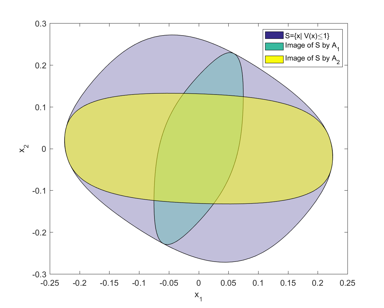 Figure 1
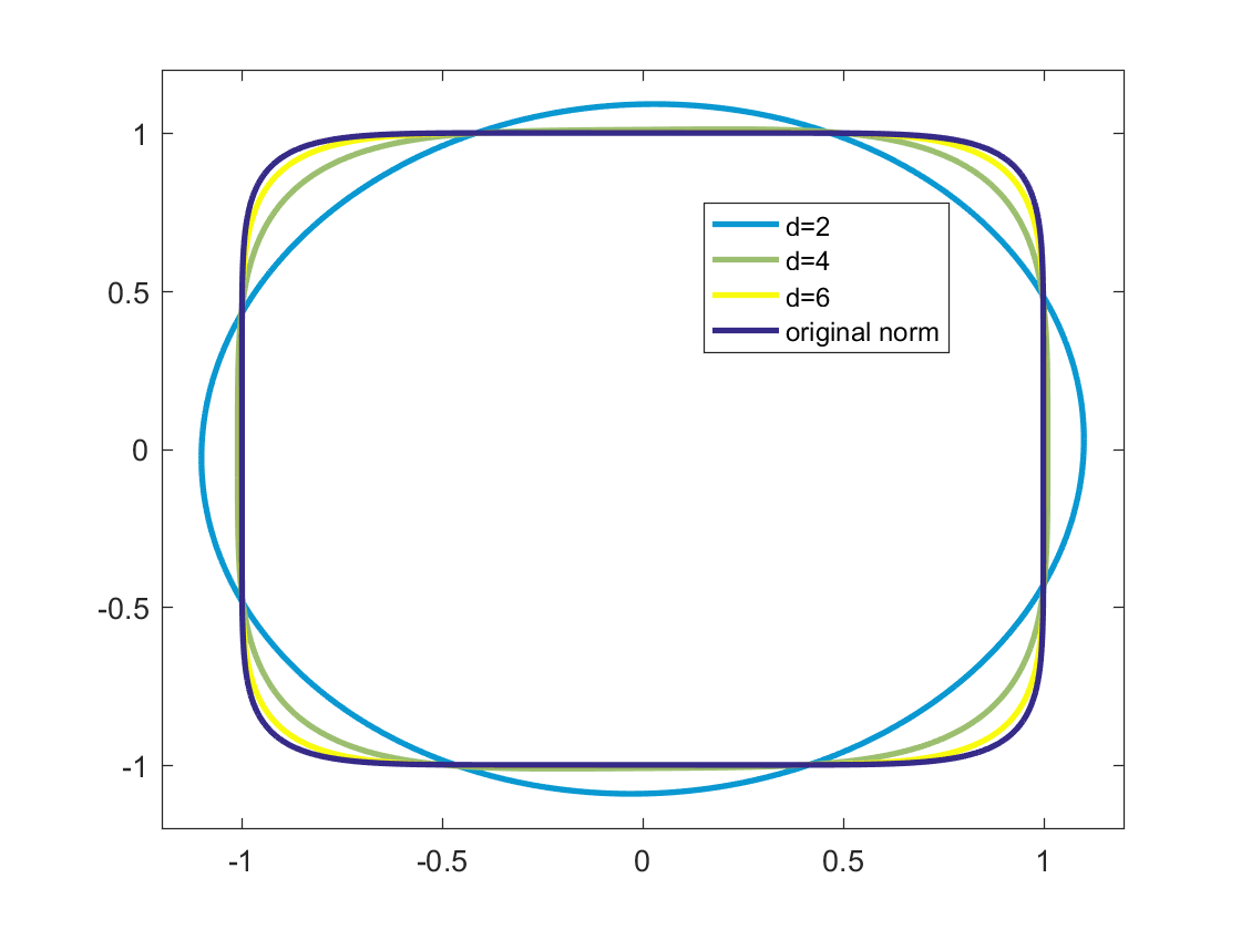 Figure 2
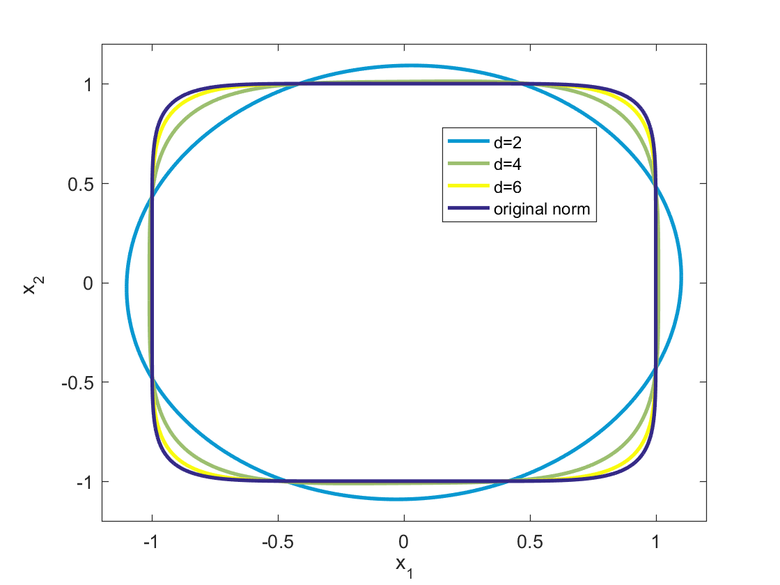 Figure 3
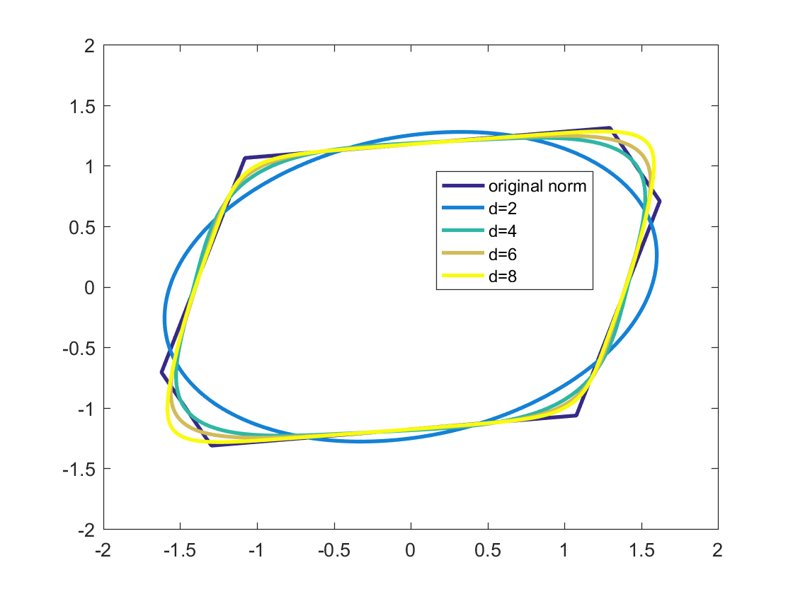 Figure 4
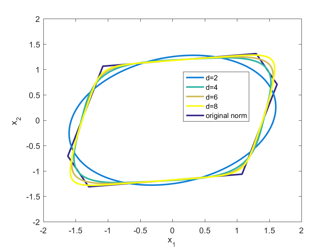 Figure 5
Peer Reviews
No public reviews on file for this paper yet. If you reviewed it on a platform where reviews are public (OpenReview, ICLR, NeurIPS, ICML), you can paste yours below so the community can read it here.
Videos
No videos yet. Explain this paper in a talk, walkthrough, or lecture? Add one.
Taxonomy
TopicsAdvanced Optimization Algorithms Research · Complexity and Algorithms in Graphs · Polynomial and algebraic computation
Polynomial Norms
Amir Ali Ahmadi 44footnotemark: 4 Amir Ali Ahmadi. ORFE, Princeton University, Sherrerd Hall, Princeton, NJ 08540, USA. Email: [email protected]
Etienne de Klerk Etienne de Klerk. Department Econometrics and Operations Research, TISEM, Tilburg University, 5000LE Tilburg, The Netherlands. Email: [email protected]
Georgina Hall Georgina Hall, corresponding author. ORFE, Princeton University, Sherrerd Hall, Princeton, NJ 08540, USA. Email: [email protected] Ali Ahmadi and Georgina Hall are partially supported by the DARPA Young Faculty Award, the Young Investigator Award of the AFOSR, the CAREER Award of the NSF, the Google Faculty Award, and the Sloan Fellowship.
Abstract
In this paper, we study polynomial norms, i.e. norms that are the root of a degree- homogeneous polynomial . We first show that a necessary and sufficient condition for to be a norm is for to be strictly convex, or equivalently, convex and positive definite. Though not all norms come from roots of polynomials, we prove that any norm can be approximated arbitrarily well by a polynomial norm. We then investigate the computational problem of testing whether a form gives a polynomial norm. We show that this problem is strongly NP-hard already when the degree of the form is 4, but can always be answered by solving a hierarchy of semidefinite programs. We further study the problem of optimizing over the set of polynomial norms using semidefinite programming. To do this, we introduce the notion of r-sos-convexity and extend a result of Reznick on sum of squares representation of positive definite forms to positive definite biforms. We conclude with some applications of polynomial norms to statistics and dynamical systems.
Keywords: polynomial norms, sum of squares polynomials, convex polynomials, semidefinite programming
AMS classification: 90C22, 14P10, 52A27
1 Introduction
A function is a norm if it satisfies the following three properties:
- (i)
positive definiteness: and . 2. (ii)
-homogeneity: . 3. (iii)
triangle inequality:
Some well-known examples of norms include the -norm, , the -norm, , and the -norm, Our focus throughout this paper is on norms that can be derived from multivariate polynomials. More specifically, we are interested in establishing conditions under which the root of a homogeneous polynomial of degree is a norm, where is an even number. We refer to the norm obtained when these conditions are met as a polynomial norm. It is straightforward to see why we restrict ourselves to roots of degree- homogeneous polynomials. Indeed, nonhomogeneous polynomials cannot hope to satisfy the homogeneity condition of a norm and homogeneous polynomials of degree are not 1-homogeneous unless we take their root. The question of when the square root of a homogeneous quadratic polynomial is a norm (i.e., when ) has a well-known answer (see, e.g., [16, Appendix A]): a function is a norm if and only if the symmetric matrix is positive definite. In the particular case where is the identity matrix, one recovers the -norm. Positive definiteness of can be checked in polynomial time using for example Sylvester’s criterion (positivity of the leading principal minors of ). This means that testing whether the square root of a quadratic form is a norm can be done in polynomial time. A similar characterization in terms of conditions on the coefficients are not known for polynomial norms generated by forms of degree greater than 2. In particular, it is not known whether one can efficiently test membership or optimize over the set of polynomial norms.
Outline and contributions.
In this paper, we study polynomial norms from a computational perspective. In Section 2, we give two different necessary and sufficient conditions under which the root of a degree- form will be a polynomial norm: namely, that be strictly convex, or (equivalently) that be convex and postive definite (Theorem 2.1). Section 3 investigates the relationship between general norms and polynomial norms: while many norms are polynomial norms (including all -norms with even), some norms are not (consider, e.g., the -norm). We show, however, that any norm can be approximated to arbitrary precision by a polynomial norm (Theorem 3.1). While it is well known that polynomials can approximate continuous functions on compact sets arbitrarily well, the approximation result here needs to preserve the convexity and homogeneity properties of the original norm, and hence does not follow, e.g., from the Stone-Weierstrass theorem. In Section 4, we move on to complexity results and show that simply testing whether the root of a quartic form is a norm is strongly NP-hard (Theorem 4.1). We then provide a semidefinite programming-based hierarchy for certifying that the root of a degree form is a norm (Theorem 4.4) and for optimizing over a subset of the set of polynomial norms (Theorem 4.21). The latter is done by introducing the concept of -sum of squares-convexity (see Definition 4.7). We show that any form with a positive definite Hessian is -sos-convex for some value of , and present a lower bound on that value (Theorem 4.8). We also show that the level of the semidefinite programming hierarchy cannot be bounded as a function of the number of variables and the degree only (Theorem 4.19). Finally, we cover some applications of polynomial norms in statistics and dynamical systems in Section 5. In Section 5.1, we compute approximations of two different types of norms, polytopic gauge norms and -norms with noneven, using polynomial norms. The techniques described in this section can be applied to norm regression. In Section 5.2, we use polynomial norms to prove stability of a switched linear system, a task which is equivalent to computing an upperbound on the joint spectral radius of a family of matrices.
2 Two equivalent characterizations of polynomial norms
We start this section with a theorem that provides conditions under which the root of a degree- form is a norm. We will use this theorem in Section 4 to establish semidefinite programming-based approximations of polynomial norms. We remark that this result is generally assumed to be known by the optimization community. Indeed, some prior work on polynomial norms has been done by Dmitriev and Reznick in [18, 19, 38, 41]. For completeness of presentation, however, and as we could not find the exact statement of this result in the form we present, we include it here with alternative proofs. Throughout this paper, we suppose that the number of variables is larger or equal than and that is a positive even integer.
Theorem 2.1**.**
Let be a form of degree in variables. The following statements are equivalent:
- (i)
The function is a norm on . 2. (ii)
The function is convex and positive definite. 3. (iii)
The function is strictly convex, i.e.,
[TABLE]
Proof.
If is a norm, then is positive definite, and so is . Furthermore, any norm is convex and the power of a nonnegative convex function remains convex.
Suppose that is convex, positive definite, but not strictly convex, i.e., there exists with , and such that
[TABLE]
Let Note that is a restriction of to a line and, consequently, is a convex, positive definite, univariate polynomial in . We now define
[TABLE]
Similarly to , is a convex univariate polynomial as it is the sum of two convex univariate polynomials. We also know that . Indeed, by convexity of , we have that and . This inequality holds in particular for and , which proves the claim. Observe now that . By convexity of and its nonnegativity over , we have that on which further implies that . Hence, from (1), is an affine function. As is positive definite, it cannot be that has a nonzero slope, so has to be a constant. But this contradicts that To see why this limit must be infinite, we show that As and , this implies that To show that , let
[TABLE]
By positive definiteness of , Let be any positive scalar and define . Then for any such that , we have
[TABLE]
where the second inequality holds by homogeneity of Thus .
Homogeneity of is immediate. Positivity follows from the first-order characterization of strict convexity:
[TABLE]
Indeed, for , the inequality becomes , as and . Hence, is positive definite, and so is . It remains to prove the triangle inequality. Let . Denote by and the 1-sublevel sets of and respectively. It is clear that
[TABLE]
and as is strictly convex (and hence quasi-convex), is convex and so is . Let We have that and . From convexity of ,
[TABLE]
Homogeneity of then gives us
[TABLE]
which shows that triangle inequality holds. ∎
3 Approximating norms by polynomial norms
It is easy to see that not all norms are polynomial norms. For example, the 1-norm is not a polynomial norm. Indeed, all polynomial norms are differentiable at all but one point (the origin) whereas the 1-norm is nondifferentiable whenever one of the components of is equal to zero. In this section, we show that, though not every norm is a polynomial norm, any norm can be approximated to arbitrary precision by a polynomial norm (Theorem 3.1). A related result is given by Barvinok in [13]. In that paper, he shows that any norm can be approximated by the -th root of a nonnegative degree- form, and quantifies the quality of the approximation as a function of and . The form he obtains however is not shown to be convex. In fact, in a later work [14, Section 2.4], Barvinok points out that it would be an interesting question to know whether any norm can be approximated by the root of a convex form with the same quality of approximation as for -th roots of nonnegative forms. The result below is a step in that direction, although the quality of approximation is weaker than that by Barvinok [13]. We note that the form in Barvinok’s construction is a sum of squares of other forms. Such forms are not necessarily convex. By contrast, the form that we construct is a sum of powers of linear forms and hence always convex.
Theorem 3.1**.**
*Let be any norm on . Then, 111We would like to thank an anonymous referee for suggesting the proof of part (i) of this theorem. We were previously showing that for any norm on and for any , there exist an even integer and an -variate positive definite form of degree , which is a sum of powers of linear forms, and such that
for any even integer :*
- (i)
There exists an -variate convex positive definite form of degree such that
[TABLE]
In particular, for any sequence of such polynomials one has
[TABLE] 2. (ii)
One may assume without loss of generality that in (i) is a nonnegative sum of powers of linear forms.
Proof of (i).
Fix any norm on . We denote the Euclidean inner product on by , and the unit ball with respect to by
[TABLE]
We denote the polar of with respect to by
[TABLE]
Recall that is symmetric around the origin, because is. One may express the given norm in terms of the polar as follows (see e.g. relation (3.1) in [13]):
[TABLE]
For given, even integer , we define the polynomial
[TABLE]
Note that is indeed a convex form of degree . In fact, we will show later on that may in fact be written as a nonnegative sum of th powers of linear forms.
By (3), one has
[TABLE]
Now fix such that . By (3), there exists a so that . Define the half-space
[TABLE]
Then, by symmetry,
[TABLE]
For any we now define
[TABLE]
Then , and
[TABLE]
Moreover
[TABLE]
and
[TABLE]
Letting , by symmetry one has , and
[TABLE]
Thus
[TABLE]
The last expression is maximized by , yielding the leftmost inequality in (2) in the statement of the theorem. Finally, note that,
[TABLE]
as required. ∎
For the proof of the second part of the theorem, we need a result concerning finite moment sequences of signed measures, given as the next lemma.
Lemma 3.2** ( [43], see Lemma 3.1 in [44] for a simple proof).**
Let be Lebesgue-measurable, and let be the normalized Lebesgue measure on , i.e. . Denote the moments of by
[TABLE]
where if and . Let be finite. Then there exists an atomic probability measure, say , supported on at most points in , such that
[TABLE]
We may now prove part 2 of Theorem 3.1.
Proof of (ii) of Theorem 3.1.
Let be the normalized Lebesgue measure on , i.e.
[TABLE]
We now use the multinomial theorem
[TABLE]
with the multinomial notation
[TABLE]
to rewrite in (4) as
[TABLE]
where is the moment of order of , as defined in (8).
By Lemma 3.2, there exist with so that
[TABLE]
for some with . Substituting in (9), one has
[TABLE]
as required. ∎
4 Semidefinite programming-based approximations of polynomial norms
4.1 Complexity
It is natural to ask whether testing if the root of a given degree- form is a norm can be done in polynomial time. In the next theorem, we show that, unless , this is not the case even when .
Theorem 4.1**.**
Deciding whether the root of a quartic form is a norm is strongly NP-hard.
Proof.
The proof of this result is adapted from a proof in [6]. Recall that the CLIQUE problem can be described thus: given a graph and a positive integer , decide whether contains a clique of size at least . The CLIQUE problem is known to be NP-hard [20]. We will give a reduction from CLIQUE to the problem of testing convexity and positive definiteness of a quartic form. The result then follows from Theorem 2.1. Let be the clique number of the graph at hand, i.e., the number of vertices in a maximum clique of . Consider the following quartic form
[TABLE]
In [6], using in part a result in [31], it is shown that
[TABLE]
is convex and is positive semidefinite. Here, is a positive constant defined as the largest coefficient in absolute value of any monomial present in some entry of the matrix . As is positive definite and as we are adding this term to a positive semidefinite expression, the resulting polynomial is positive definite. Hence, the equivalence holds if and only if the quartic on the righthandside of the equivalence in (10) is convex and positive definite. ∎
Note that this also shows that strict convexity is hard to test for quartic forms (this is a consequence of Theorem 2.1). A related result is Proposition 3.5. in [6], which shows that testing strict convexity of a polynomial of even degree is hard. However, this result is not shown there for forms, hence the relevance of the previous theorem.
Theorem 4.1 rules out the possibility of a pseudo-polynomial time characterization of polynomial norms (unless P=NP) and motivates the study of tractable sufficient conditions. The sufficient conditions we consider next are based on semidefinite programming. Semidefinite programs can be solved to arbitrary accuracy in polynomial time [45] and technology for solving this class of problems is rapidly improving [9, 34, 30, 46, 21, 42, 5].
4.2 Sum of squares polynomials and semidefinite programming review
We start this section by reviewing the notion of sum of squares polynomials and related concepts such as sum of squares-convexity. We say that a polynomial is a sum of squares (sos) if , for some polynomials . Being a sum of squares is a sufficient condition for being nonnegative. The converse however is not true, as is exemplified by the Motzkin polynomial
[TABLE]
which is nonnegative but not a sum of squares [33]. The sum of squares condition is a popular surrogate for nonnegativity due to its tractability. Indeed, while testing nonnegativity of a polynomial of degree greater or equal to 4 is a hard problem, testing whether a polynomial is a sum of squares can be done using semidefinite programming. This comes from the fact that a polynomial of degree is a sum of squares if and only if there exists a positive semidefinite matrix such that , where is the standard vector of monomials of degree up to (see, e.g., [35]). As a consequence, any optimization problem over the coefficients of a set of polynomials which includes a combination of affine constraints and sos constraints on these polynomials, together with a linear objective can be recast as a semidefinite program. These type of optimization problems are known as sos programs and have found widespread applications in recent years [36, 29, 25, 24].
Though not all nonnegative polynomials can be written as sums of squares, the following theorem by Artin [10] circumvents this problem using sos multipliers.
Theorem 4.2** (Artin [10]).**
For any nonnegative polynomial , there exists an sos polynomial such that is sos.
This theorem in particular implies that if we are given a polynomial , then we can always check its nonnegativity using an sos program that searches for (of a fixed degree). However, this result does not allow us to optimize over the set of nonnegative polynomials or positive semidefinite polynomial matrices using an sos program (as far as we know). This is because, in that setting, products of decision varibles arise from multiplying polynomials and , whose coefficients are decision variables.
By adding further assumptions on , Reznick showed in [39] that one could further pick to be a power of (we refer the reader to [12, Chapter 1, Section 3] for another nice presentation of Reznick’s result). In what follows, denotes the unit sphere in
Theorem 4.3** (Reznick [39]).**
Let be a positive definite form of degree in variables and define
[TABLE]
If , then is a sum of squares.
Motivated by this theorem, the notion of -sos polynomials can be defined: a polynomial is said to be -sos if is sos. Note that it is clear that any -sos polynomial is nonnegative and that the set of -sos polynomials is included in the set of -sos polynomials. The Motzkin polynomial in (11) for example is -sos although not sos.
To end our review, we briefly touch upon the concept of sum of squares-convexity (sos-convexity), which we will build upon in the rest of the section. Let denote the Hessian matrix of a polynomial . We say that is sos-convex if is a sum of squares (as a polynomial in and ). As before, optimizing over the set of sos-convex polynomials can be cast as a semidefinite program. Sum of squares-convexity is obviously a sufficient condition for convexity via the second-order characterization of convexity. However, there are convex polynomials which are not sos-convex (see, e.g., [7]). For a more detailed overview of sos-convexity including equivalent characterizations and settings in which sos-convexity and convexity are equivalent, refer to [8].
4.2.1 Notation
Throughout, we will use the notation (resp. ) to denote the set of forms (resp. positive semidefinite, aka nonnegative, forms) in variables and of degree . We will futhermore use the falling factorial notation and for a positive integer .
4.3 Certifying validity of a polynomial norm
In this subsection, we assume that we are given a form of degree and we would like to prove that is a norm using semidefinite programming.
Theorem 4.4**.**
Let be a degree- form. Then is a polynomial norm if and only if there exist , , and an sos form such that is sos and is sos. Furthermore, this condition can be checked using semidefinite programming.
To show this result, we require a counterpart to Theorem 4.2 for matrices, which we present below. We say that a polynomial matrix , i.e., a matrix whose entries are polynomials in , is positive semidefinite if it has nonnegative eigenvalues for all substitutions .
Proposition 4.5** ([37, 22, 27]).**
If is a positive semidefinite polynomial matrix, then there exists a sum of squares polynomial such that is a sum of squares.
Proof.
This is an immediate consequence of a theorem by Procesi and Schacher [37] and independently Gondard and Ribenboim [22], reproven by Hillar and Nie [27]. This theorem states that if is a symmetric polynomial matrix that is positive semidefinite for all then
[TABLE]
where the matrices are symmetric and have rational functions as entries. Let be the polynomial obtained by multiplying all denominators of the rational functions involved in any of the matrices . Note that is a sum of squares as
[TABLE]
However, is now a matrix with polynomial entries, which gives the result. ∎
We remark that this result does not immediately follow from the theorem given by Artin as the multiplier does not depend on and , but solely on . We now prove Theorem 4.4.
Proof of Theorem 4.4.
It is immediate to see that if there exist such a , , and , then is convex and positive definite. From Theorem 2.1, this means that is a polynomial norm.
Conversely, if is a polynomial norm, then, by Theorem 2.1, is convex and positive definite. As is convex, the polynomial is nonnegative. Using Proposition 4.5, we conclude that there exists an sos polynomial such that is sos. We now show that, as is positive definite, there exist and such that is sos. Let denote the minimum of on the sphere. As is positive definite, We take and consider . We have that is a positive definite form: indeed, if is a nonzero vector in , then
[TABLE]
by homogeneity of and definition of . Using Theorem 4.3, such that is sos.
For fixed , a given form , and a fixed degree , one can search for and an sos form of degree such that is sos and is sos using semidefinite programming. This is done by solving the following semidefinite feasibility problem:
[TABLE]
where the unknowns are the coefficients of and the real number . ∎
Remark 4.6**.**
We remark that we are not imposing in the semidefinite program above. This is because, in practice, especially if the semidefinite program is solved with interior point methods, the solution returned by the solver will be in the interior of the feasible set, and hence will automatically be positive. One can slightly modify (12) however to take the constraint into consideration explicitly. Indeed, consider the following semidefinite feasibility problem where both the degree of and the integer are fixed:
[TABLE]
It is easy to check that (13) is feasible with if and only if the last constraint of (12) is feasible with . To see this, take and note that can never be zero.
To the best of our knowledge, we cannot use the approach described in Theorem 4.4 to optimize over the set of polynomial norms with a semidefinite program. This is because of the product of decision variables in the coefficients of and . The next subsection will address this issue.
4.4 Optimizing over the set of polynomial norms
In this subsection, we consider the problem of optimizing over the set of polynomial norms. To do this, we introduce the concept of -sos-convexity. Recall that the notation references the Hessian matrix of a form .
4.4.1 Positive definite biforms and r-sos-convexity
Definition 4.7**.**
For an integer , we say that a polynomial is -sos-convex if is sos.
Observe that, for fixed , the property of -sos-convexity can be checked using semidefinite programming (though the size of this SDP gets larger as increases). Any polynomial that is -sos-convex is convex. Note that the set of -sos-convex polynomials is a subset of the set of -sos-convex polynomials and that the case corresponds to the set of sos-convex polynomials. We remark that in Theorem 3.1 is in fact sos-convex, since it is a sum of squares of linear forms. Thus Theorem 3.1 implies that any norm on may be approximated arbitrarily well by a polynomial norm that corresponds to a sos-convex form.
It is natural to ask whether any convex polynomial is -sos-convex for some . Our next theorem shows that this is the case provided that the biform , where is the Hessian of , is positive over the bi-sphere.
Theorem 4.8**.**
Let be a form of degree such that for . Let
[TABLE]
If , then is -sos-convex.
Remark 4.9**.**
Note that can also be interpreted as
[TABLE]
Remark 4.10**.**
Theorem 4.8 is a generalization of Theorem 4.3 by Reznick. Note though that this is not an immediate generalization. First, is not a positive definite form (consider, e.g., and any nonzero ). Secondly, note that the multiplier is and does not involve the variables. (As we will see in the proof, this is essentially because is quadratic in .) It is not immediate that the multiplier should have this specific form. From Theorem 4.3, it may perhaps seem more natural that the multiplier be . It turns out in fact that such a multiplier would not give us the correct property (contrarily to ) as there exist forms whose Hessian is positive definite for all but for which the form
[TABLE]
is not sos for any . For a specific example, consider the form in variables and of degree given in [7, Theorem 3.2]. It is shown in [7] that (i) is convex; (ii) the entry of the Hessian of , , is not sos; and (iii) is sos.
Suppose for the sake of contradiction that
[TABLE]
is sos for some . This implies that the polynomial
[TABLE]
should be sos for any as it is obtained from by setting . Expanding this out, we get
[TABLE]
From arguments (ii) and (iii) above, we know that is not sos but
[TABLE]
is sos. Fixing large enough, we can ensure that is not sos. This contradicts our previous assumption.
Remark 4.11**.**
Theorem 4.8 can easily be adapted to biforms of the type where ’s are forms of degree in and ’s are forms of degree in . In this case, there exist integers such that
[TABLE]
is sos. For the purposes of this paper however and the connection to polynomial norms, we will show the result in the particular case where the biform of interest is
We associate to any form , the -th order differential operator , defined by replacing each occurence of with . For example, if where and , then its differential operator will be
[TABLE]
Our proof will follow the structure of the proof of Theorem 4.3 given in [39] and reutilize some of the results given in the paper which we quote here for clarity of exposition.
Proposition 4.12** ([39], see Proposition 2.6).**
For any nonnegative integer , there exist nonnegative rationals and integers such that
[TABLE]
For simplicity of notation, we will let and . Hence, we will write to mean .
Proposition 4.13** ([39], see Proposition 2.8).**
If and , then
[TABLE]
Proposition 4.14** ([39], see Theorems 3.7 and 3.9).**
For and , we define by
[TABLE]
The inverse of exists and this is a map verifying
Proposition 4.15** ([39], see Theorem 3.12 ).**
Suppose is a positive definite form in variables and of degree and let
[TABLE]
If , then
We will focus throughout the proof on biforms of the following structure
[TABLE]
where , for all , and some even integer . Note that the polynomial (where is some form) has this structure. We next present three lemmas which we will then build on to give the proof of Theorem 4.8.
Lemma 4.16**.**
For a biform of the structure in (15), define the operator as
[TABLE]
If is positive semidefinite (i.e., ), then, for any , the biform
[TABLE]
is a sum of squares.
Proof.
Using Proposition 4.12, we have
[TABLE]
where and Hence, applying Proposition 4.13, we get
[TABLE]
Notice that is a quadratic form in which is positive semidefinite by assumption, which implies that it is a sum of squares (as a polynomial in ). Furthermore, as and is an even power of a linear form, we have that is a sum of squares (as a polynomial in ). Combining both results, we get that (16) is a sum of squares. ∎
We now extend the concept introduced by Reznick in Proposition 4.14 to biforms.
Lemma 4.17**.**
For a biform of the structure as in (15), we define the biform as
[TABLE]
where is as in (14). Define
[TABLE]
where is the inverse of . Then, we have
[TABLE]
and
[TABLE]
Proof.
We start by showing that (17) holds:
[TABLE]
We now show that (18) holds:
[TABLE]
∎
Lemma 4.18**.**
For a biform of the structure in (15), which is positive on the bisphere, let
[TABLE]
If , then is positive semidefinite.
Proof.
Fix and consider , which is a positive definite form in of degree . From Proposition 4.15, if
[TABLE]
then is positive semidefinite. As for any , we have that if
[TABLE]
then is positive semidefinite, regardless of the choice of Hence, is positive semidefinite (as a function of and ).
∎
Proof of Theorem 4.8.
Let , let , and let
[TABLE]
We know by Lemma 4.18 that is positive semidefinite. Hence, using Lemma 4.16, we get that
[TABLE]
is sos. Lemma 4.17 then gives us:
[TABLE]
As a consequence, is sos.
∎
The last theorem of this section shows that one cannot bound the integer in Theorem 4.8 as a function of and only.
Theorem 4.19**.**
For any integer , there exists a form in 3 variables and of degree 8 such that , but is not -sos-convex.
Proof.
Consider the trivariate octic:
[TABLE]
It is shown in [7] that has positive definite Hessian, and that the entry of , which we will denote by , is 1-sos but not sos. We will show that for any , one can find such that
[TABLE]
satisfies the conditions of the theorem.
We start by showing that for any , has positive definite Hessian. To see this, note that for any , we have:
[TABLE]
As for any , this is in particular true when and when , which gives us that the Hessian of is positive definite for any
We now show that for a given , there exists such that is not sos. We use the following result from [40, Theorem 1]: for any positive semidefinite form which is not sos, and any , there exists such that is not sos. As is 1-sos but not sos, we can apply the previous result. Hence, there exists a positive integer such that
[TABLE]
is not sos. This implies that is not sos. Indeed, if was sos, then would be sos with But, we have
[TABLE]
which is not sos. Hence, is not sos, and is not -sos-convex. ∎
Remark 4.20**.**
Any form with is strictly convex but the converse is not true.
To see this, note that any form of degree with a positive definite Hessian is convex (as ) and positive definite (as, from a recursive application of Euler’s theorem on homogeneous functions, ). From the proof of Theorem 2.1, this implies that is strictly convex.
To see that the converse statement is not true, consider the strictly convex form . We have
[TABLE]
which is not positive definite e.g., when .
4.4.2 Optimizing over a subset of polynomial norms with -sos-convexity
In the following theorem, we give a semidefinite programming-based hierarchy for optimizing over the set of forms with , Comparatively to Theorem 4.4, this theorem allows us to impose as a constraint that the root of a form be a norm, rather than simply testing whether it is. This comes at a cost however: in view of Remark 4.20 and Theorem 2.1, we are no longer considering all polynomial norms, but a subset of them whose power has a positive definite Hessian.
Theorem 4.21**.**
Let be a degree- form. Then if and only if such that is -sos-convex. Furthermore, this condition can be imposed using semidefinite programming.
Proof.
If there exist such that is -sos-convex, then , As the Hessian of is positive definite for any nonzero and as , we get ,
Conversely, if , , then on the bisphere (and conversely). Let
[TABLE]
We know that is attained and is positive. Take and consider
[TABLE]
Then
[TABLE]
Note that, by Cauchy-Schwarz, we have . If , we get
[TABLE]
Hence, and there exists such that is -sos-convex from Theorem 4.8.
For fixed , the condition that there be such that is -sos-convex can be imposed using semidefinite programming. This is done by searching for coefficients of a polynomial and a real number such that
[TABLE]
Note that both of these conditions can be imposed using semidefinite programming. ∎
Remark 4.22**.**
Note that we are not imposing in the above semidefinite program. As mentioned in Section 4.3, this is because in practice the solution returned by interior point solvers will be in the interior of the feasible set.
In the special case where is completely free222This is the case of our two applications in Section 5. (i.e., when there are no additional affine conditions on the coefficients of ), one can take in (19) instead of . Indeed, if there exists , an integer , and a polynomial such that is -sos-convex, then will be a solution to (19) with replacing .
5 Applications
5.1 Norm approximation and regression
In this section, we study the problem of approximating a (non-polynomial) norm by a polynomial norm. We consider two different types of norms: -norms with noneven (and greater than 1) and gauge norms with a polytopic unit ball. For -norms, we use as an example . For our polytopic gauge norm, we randomly generate an origin-symmetric polytope and produce a norm whose 1-sublevel corresponds to that polytope. This allows us to determine the value of the norm at any other point by homogeneity (see [16, Exercise 3.34] for more information on gauge norms, i.e., norms defined by convex, full-dimensional, origin-symmetric sets). To obtain our approximations, we proceed in the same way in both cases. We first sample points uniformly at random on the sphere . We then solve the following optimization problem with fixed:
[TABLE]
Problem (20) can be written as a semidefinite program as the objective is a convex quadratic in the coefficients of and the constraint has a semidefinite representation as discussed in Section 4.2. The solution returned is guaranteed to be convex. Moreover, any sos-convex form is sos (see [23, Lemma 8]), which implies that is nonnegative. One can numerically check to see if the optimal polynomial is in fact positive definite (for example, by checking the eigenvalues of the Gram matrix of a sum of squares decomposition of ). If that is the case, then, by Theorem 2.1, is a norm. Futhermore, note that we have
[TABLE]
where the first inequality is a consequence of concavity of and the second is a consequence of the inequality . This implies that if the optimal value of (20) is equal to , then the sum of the squared differences between and over the sample is less than or equal to .
It is worth noting that in our example, we are actually searching over the entire space of polynomial norms of a given degree. Indeed, as is bivariate, it is convex if and only if it is sos-convex [8]. In Figure 1, we have drawn the 1-level sets of the initial norm (either the -norm or the polytopic gauge norm) and the optimal polynomial norm obtained via (20) with varying degrees . Note that when increases, the approximation improves.
A similar method could be used for norm regression. In this case, we would have access to data points corresponding to noisy measurements of an underlying unknown norm function. We would then solve the same optimization problem as the one given in (20) to obtain a polynomial norm that most closely approximates the noisy data.
5.2 Joint spectral radius and stability of linear switched systems
As a second application, we revisit a result from one of the authors and Jungers from [1, 3] on finding upper bounds on the joint spectral radius of a finite set of matrices. We first review a few notions relating to dynamical systems and linear algebra. The spectral radius of a matrix is defined as
[TABLE]
The spectral radius happens to coincide with the eigenvalue of of largest magnitude. Consider now the discrete-time linear system , where is the state vector of the system at time . This system is said to be asymptotically stable if for any initial starting state , when A well-known result connecting the spectral radius of a matrix to the stability of a linear system states that the system is asymptotically stable if and only if .
In 1960, Rota and Strang introduced a generalization of the spectral radius to a set of matrices. The joint spectral radius (JSR) of a set of matrices is defined as
[TABLE]
Analogously to the case where we have just one matrix, the value of the joint spectral radius can be used to determine stability of a certain type of system, called a switched linear system. A switched linear system models an uncertain and time-varying linear system, i.e., a system described by the dynamics
[TABLE]
where the matrix varies at each iteration within the set . As done previously, we say that a switched linear system is asymptotically stable if when , for any starting state and any sequence of products of matrices in . One can establish that the switched linear system is asymptotically stable if and only if [28].
Switched linear systems are typically used to model situations where the dynamics of a system are thought to be linear, but the matrix associated to the linear dynamics is unknown and time-varying. Consider, e.g., the task of stabilizing a drone in a windy environment. By linearizing its dynamics around a desired equilibrium point, the behavior of the drone can be modeled locally by a linear dynamical system. However, as this linear dynamical system is unknown due to parameter uncertainty and modeling error, and time-varying due to the effect of the wind, the drone’s behavior is better modeled by a switched linear system.
Consequently, a natural question is whether one can efficiently test if and hence determine if the corresponding switched linear system is asymptotically stable. Unlike the setting of linear systems, where one can decide whether the spectral radius of a matrix is less than one in polynomial time, it is not known whether the problem of testing if is even decidable. The related question of testing whether is known to be undecidable, already when contains only 2 matrices [15]. With this result in mind, it comes as no surprise that, e.g., stability of a switched linear system is not implied by all individual matrices in having spectral radius less than one. This is easy to see on an example: consider the set of matrices given by
[TABLE]
Observe that the spectral radii of and are zero, which is less than one. However
[TABLE]
and so is lower bounded by , and the switched linear system is not stable.
An active area of research has consequently been to obtain sufficient conditions for the JSR to be strictly less than one, which, for example, can be checked using convex optimization. The theorem that we revisit below is a result of this type. We start first by recalling a classical theorem regarding stability of a linear system.
Theorem 5.1** (see, e.g., Theorem 8.4 in [26]).**
Let . Then, if and only if there exists a contracting quadratic norm; i.e., a function of the form with , such that
The next theorem (from [1, 3]) can be viewed as an extension of Theorem 5.1 to the joint spectral radius of a finite set of matrices. It is known that the existence of a contracting quadratic norm is no longer necessary for stability in this case. This theorem shows however that the existence of a contracting polynomial norm is.
Theorem 5.2** (adapted from [1, 3], Theorem 3.2 ).**
Let be a family of matrices. Then, if and only if there exists a contracting polynomial norm; i.e., a function , where is an n-variate sos-convex and positive definite form of degree , such that and
We remark that in [2], the authors show that the degree of cannot be bounded as a function of and . This is expected from the undecidability result mentioned before.
Example 5.3**.**
We consider a modification of Example 5.4. in [4] as an illustration of the previous theorem. We would like to show that the joint spectral radius of the two matrices
[TABLE]
is strictly less that one.
To do this, we search for a nonzero form of degree such that
[TABLE]
If problem (23) is feasible for some , then . A quick computation using the software package YALMIP [32] and the SDP solver MOSEK [9] reveals that, when or , problem (23) is infeasible. When however, the problem is feasible and we obtain a polynomial norm whose 1-sublevel set is the outer set plotted in Figure 2. We also plot on Figure 2 the images of this 1-sublevel set under and . Note that both sets are included in the 1-sublevel set of as expected. From Theorem 5.2, the existence of a polynomial norm implies that and hence, the pair is asymptotically stable.
Remark 5.4**.**
As mentioned previously, problem (23) is infeasible for . Instead of pushing the degree of up to 6, one could wonder whether the problem would have been feasible if we had asked that of degree be -sos-convex for some fixed . As mentioned before, in the particular case where (which is the case at hand here), the notions of convexity and sos-convexity coincide; see [8]. As a consequence, one can only hope to make problem (23) feasible by increasing the degree of .
6 Future directions
In this paper, we provided semidefinite programming-based hierarchies for certifying that the root of a given degree- form is a polynomial norm (Section 4.3), and for optimizing over the set of forms with positive definite Hessians (Section 4.4). A clear gap emerged between forms which are strictly convex and those which have a positive definite Hessian, the latter being a sufficient (but not necessary) condition for the former. This leads us to consider the following two open problems.
Open Problem 1**.**
Does there exist a family of cones that have the following two properties: (i) for each , optimization of a linear function over can be carried out with semidefinite programming, and (ii) every strictly convex form in variables and degree belongs to for some ? We have shown a weaker result, namely the existence of a family of cones that verify (i) and a modified version of (ii), where strictly convex forms are replaced by forms with a positive definite Hessian.
Open Problem 2**.**
Helton and Nie have shown in [23] that one can optimize a linear function over sublevel sets of forms that have positive definite Hessians with semidefinite programming. Is the same statement true for sublevel sets of all polynomial norms?
On the application side, it might be interesting to investigate how one can use polynomial norms to design regularizers in machine learning applications. Indeed, a very popular use of norms in optimization is as regularizers, with the goal of imposing additional structure (e.g., sparsity or low rank) on optimal solutions. One could imagine using polynomial norms to design regularizers that are based on the data at hand in place of more generic regularizers such as the 1-norm. Regularizer design is a problem that has already been considered (see, e.g., [11, 17]) but not using polynomial norms. This can be worth exploring as we have shown that polynomial norms can approximate any norm with arbitrary accuracy, while remaining differentiable everywhere (except at the origin), which can be beneficial for optimization purposes.
Acknowledgement
The authors would like to thank an anonymous referee for suggesting the proof of the first part of Theorem 3.1, which improves our previous statement by quantifying the quality of the approximation as a function of and , and two other anonymous referees for constructive comments that considerably helped improve the draft.
The reference list from the paper itself. Each links out to its DOI / PubMed record.
- 1[1] A. A. Ahmadi and R. M. Jungers, SOS-convex Lyapunov functions with applications to nonlinear switched systems , Proceedings of the IEEE Conference on Decision and Control, 2013.
- 2[2] A. A. Ahmadi and R. M. Jungers, Lower bounds on complexity of Lyapunov functions for switched linear systems , Nonlinear Analysis: Hybrid Systems 21 (2016), 118–129.
- 3[3] A. A. Ahmadi and R. M. Jungers, SOS-convex Lyapunov functions and stability of nonlinear difference inclusions , (2018), In preparation.
- 4[4] A. A. Ahmadi, R. M. Jungers, P. A. Parrilo, and M. Roozbehani, Analysis of the joint spectral radius via lyapunov functions on path-complete graphs , Proceedings of the 14th international conference on Hybrid systems: computation and control, ACM, 2011, pp. 13–22.
- 5[5] A. A. Ahmadi and A. Majumdar, DSOS and SDSOS optimization: more tractable alternatives to sum of squares and semidefinite optimization , Available at ar Xiv:1706.02586 (2017).
- 6[6] A. A. Ahmadi, A. Olshevsky, P. A. Parrilo, and J. N. Tsitsiklis, NP-hardness of deciding convexity of quartic polynomials and related problems , Mathematical Programming 137 (2013), no. 1-2, 453–476.
- 7[7] A. A. Ahmadi and P. A. Parrilo, A convex polynomial that is not sos-convex , Mathematical Programming 135 (2012), no. 1-2, 275–292.
- 8[8] , A complete characterization of the gap between convexity and sos-convexity , SIAM Journal on Optimization 23 (2013), no. 2, 811–833, Also available at ar Xiv:1111.4587.