Mass-Imbalanced Ionic Hubbard Chain
Michael Sekania, Dionys Baeriswyl, Luka Jibuti, George I. Japaridze

TL;DR
This paper studies a one-dimensional mass-imbalanced ionic Hubbard model, revealing how charge and spin orderings evolve with interaction strength and identifying a weakly first-order phase transition.
Contribution
It introduces a mean-field analysis of a combined mass-imbalanced and ionic Hubbard model, detailing phase transitions and order parameters in the ground state.
Findings
Charge order dominates at low U
Magnetic order dominates at high U
Phase transition at critical U_c
Abstract
A repulsive Hubbard model with both spin-asymmetric hopping () and a staggered potential (of strength ) is studied in one dimension. The model is a compound of the mass-imbalanced (, ) and ionic (, ) Hubbard models, and may be realized by cold atoms in engineered optical lattices. We use mostly mean-field theory to determine the phases and phase transitions in the ground state for a half-filled band (one particle per site). We find that a period-two modulation of the particle (or charge) density and an alternating spin density coexist for arbitrary Hubbard interaction strength, . The amplitude of the charge modulation is largest at , decreases with increasing and tends to zero for . The amplitude for spin alternation…
Click any figure to enlarge with its caption.
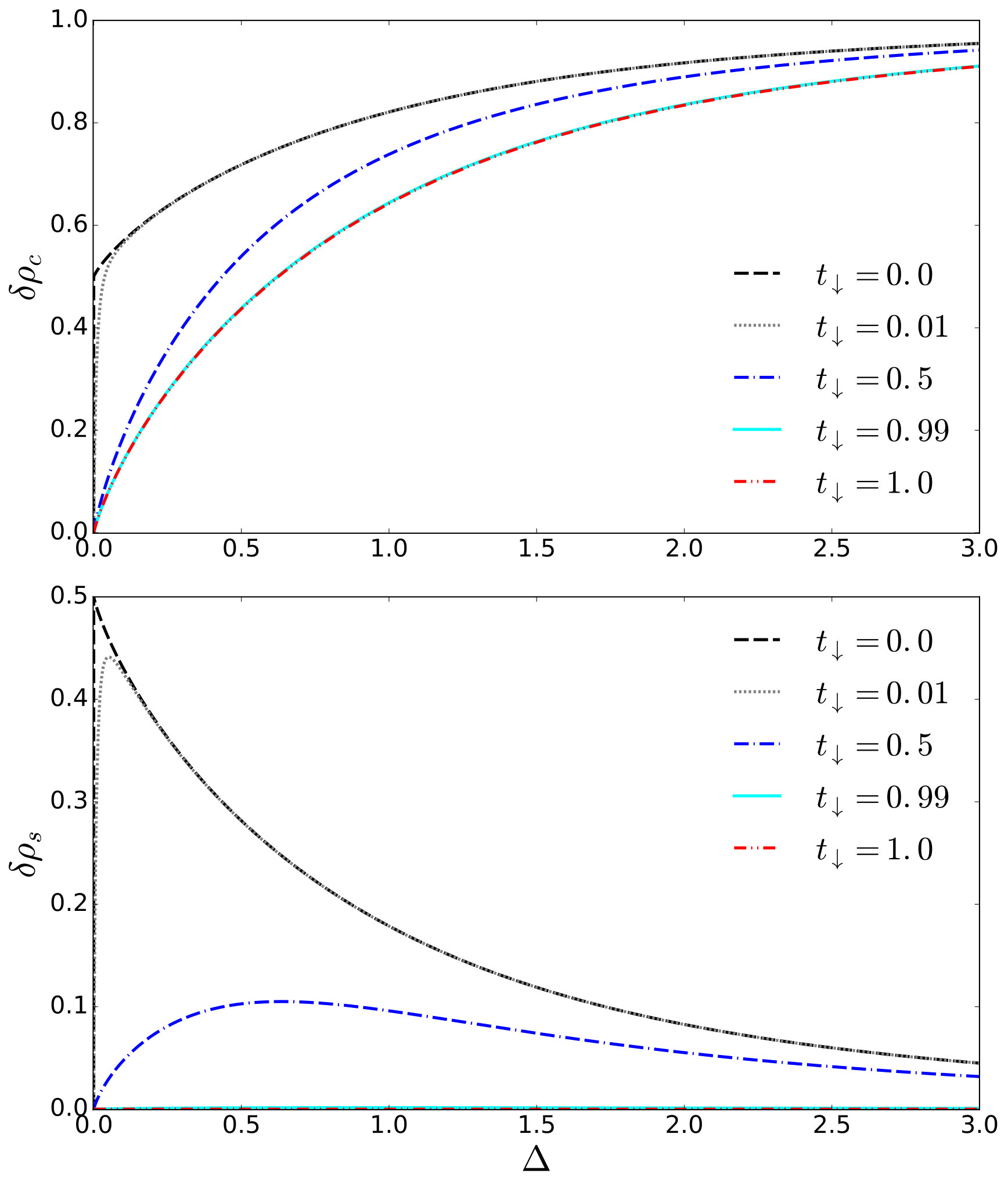 Figure 1
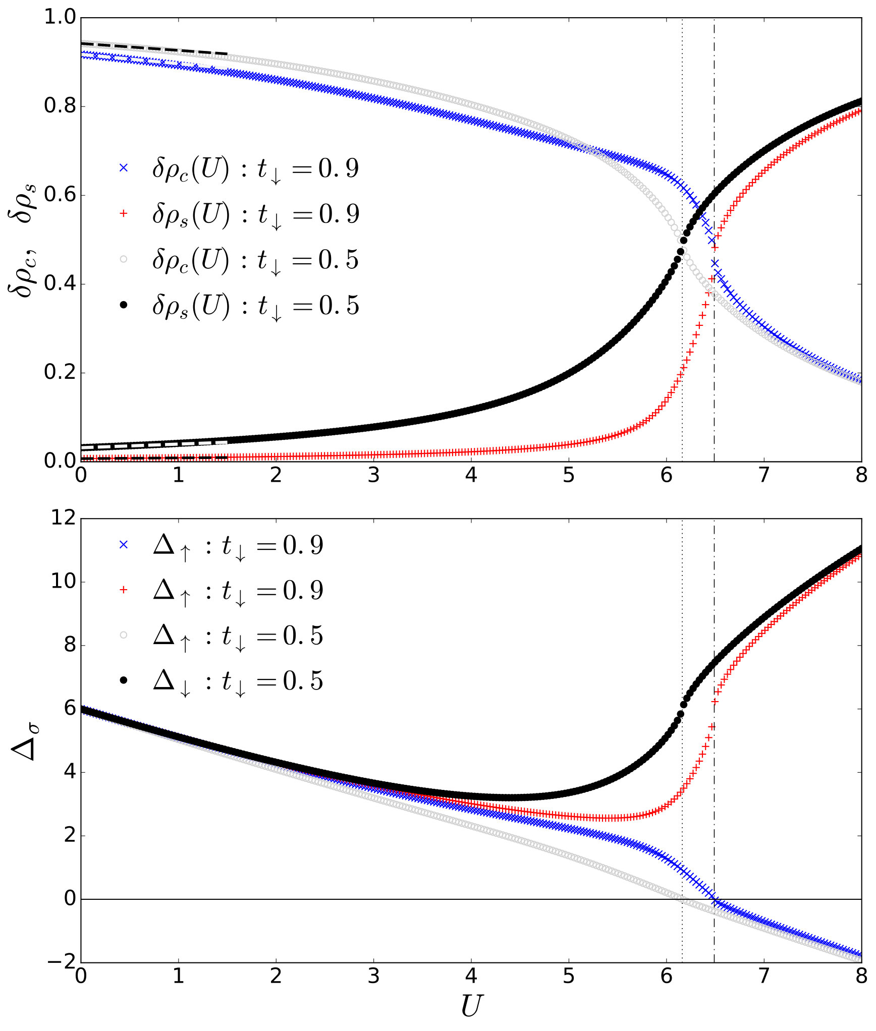 Figure 2
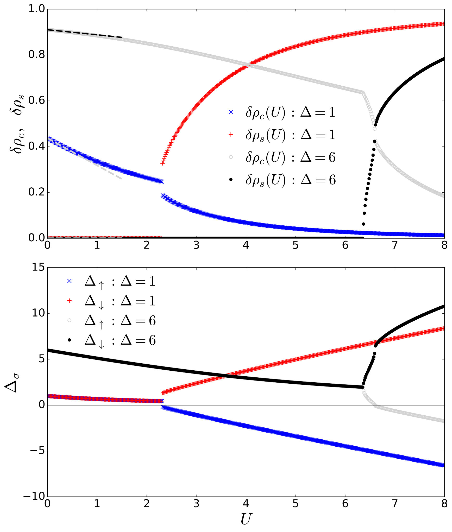 Figure 3
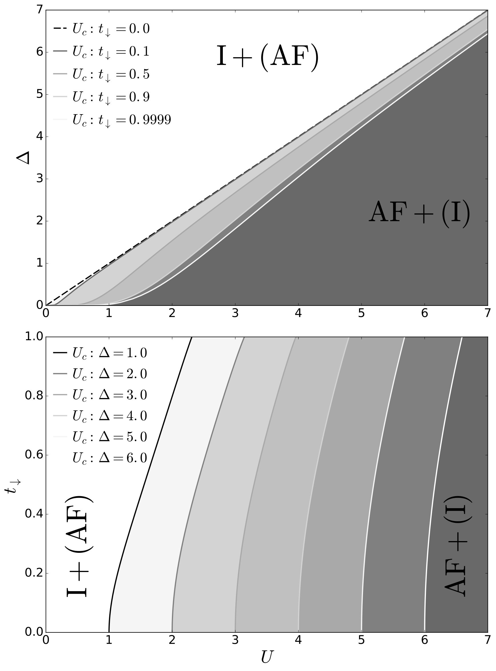 Figure 4
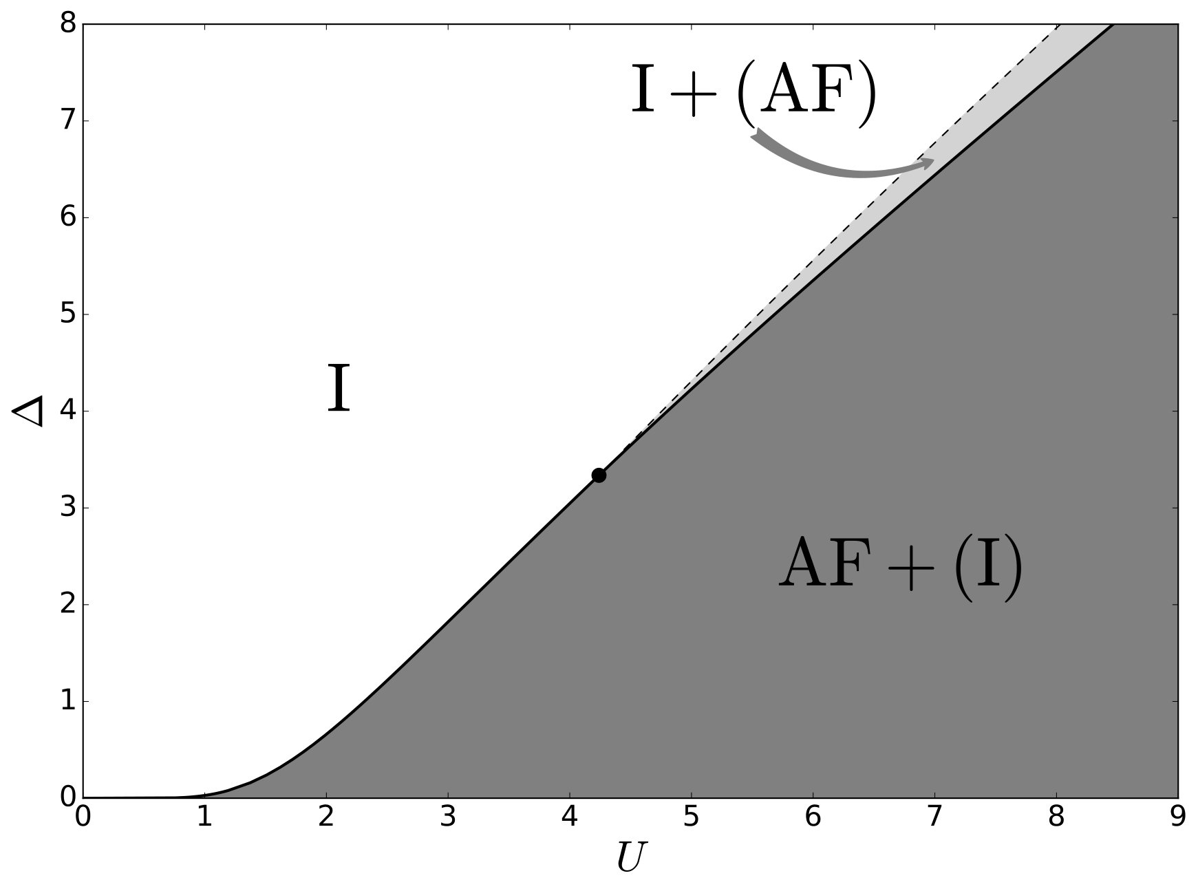 Figure 5
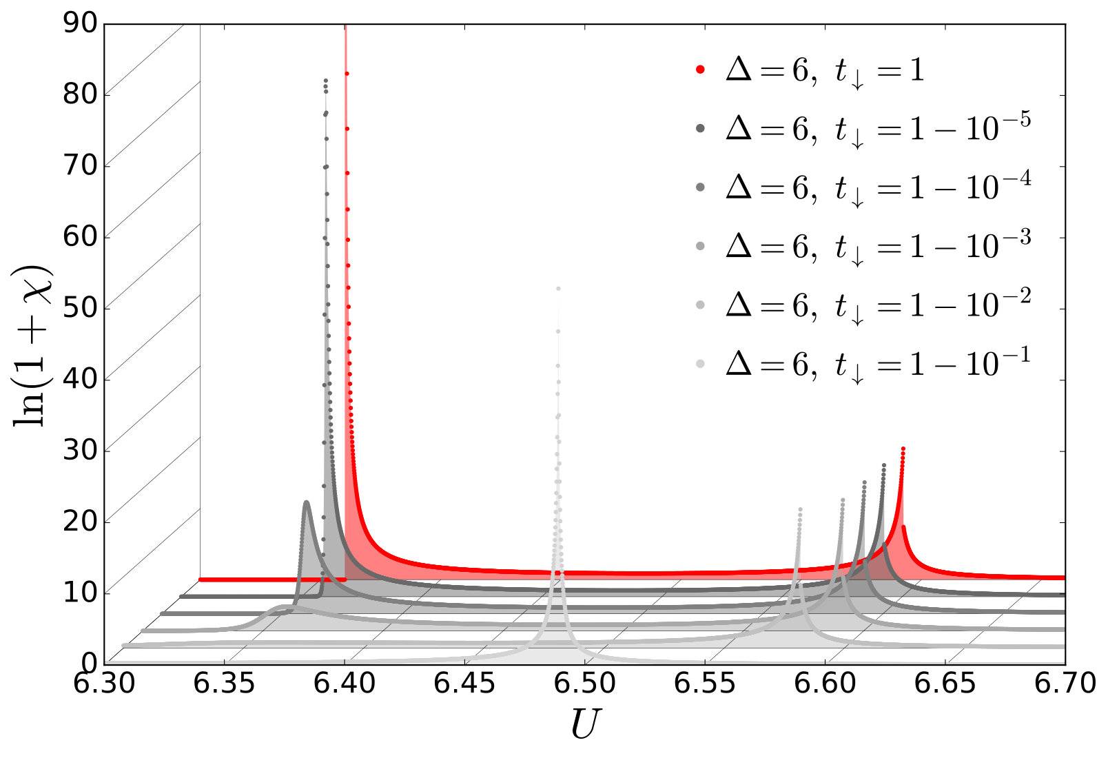 Figure 6
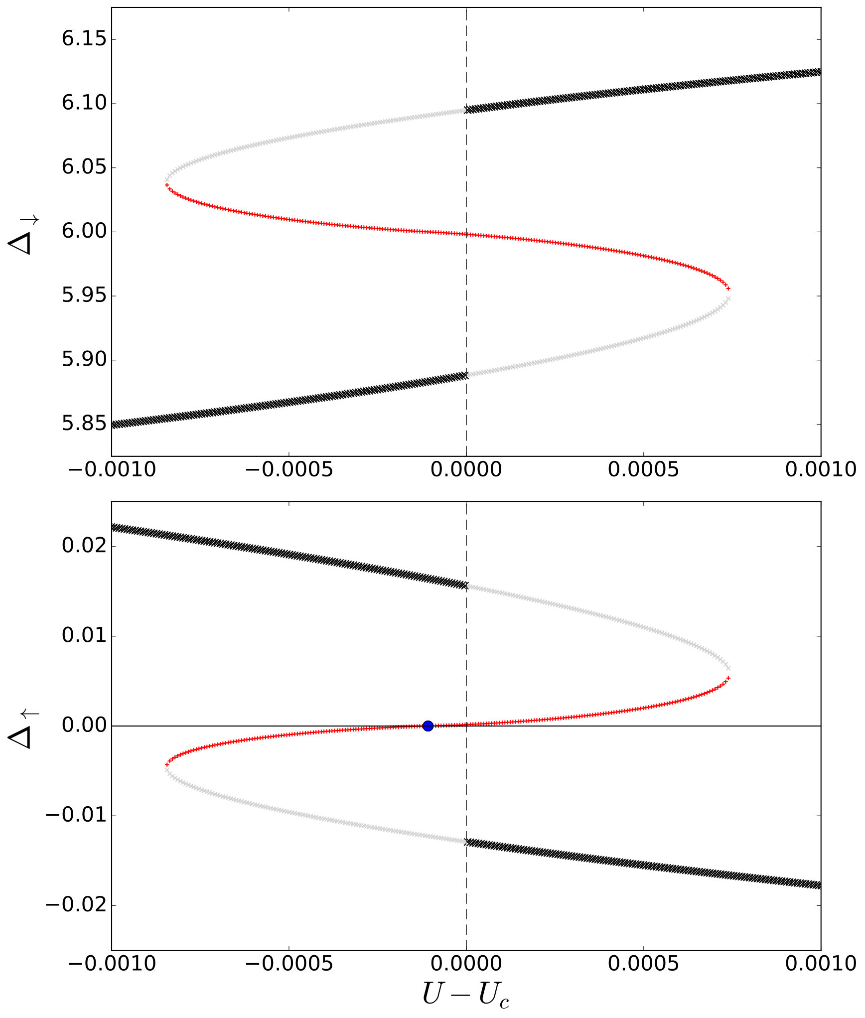 Figure 7
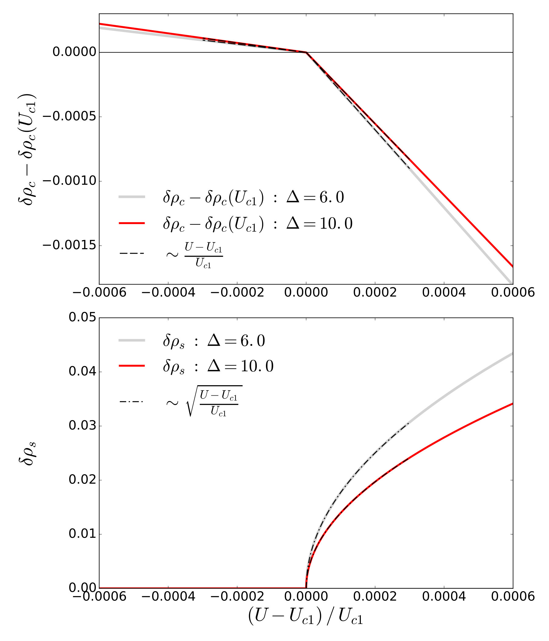 Figure 8
Peer Reviews
No public reviews on file for this paper yet. If you reviewed it on a platform where reviews are public (OpenReview, ICLR, NeurIPS, ICML), you can paste yours below so the community can read it here.
Videos
No videos yet. Explain this paper in a talk, walkthrough, or lecture? Add one.
Mass-Imbalanced Ionic Hubbard Chain
Michael Sekania
Theoretical Physics III, Center for Electronic Correlations and Magnetism, Institute of Physics,
University of Augsburg, D-86135 Augsburg, Germany
Javakhishvili Tbilisi State University, Andronikashvili Institute of Physics, Tamarashvili str. 6, 0177 Tbilisi, Georgia
Dionys Baeriswyl
Department of Physics, University of Fribourg, Chemin du Musée 3, CH-1700 Fribourg, Switzerland
International Institute of Physics, 59078-400 Natal-RN, Brazil
Luka Jibuti
Faculty of Natural Sciences and Engineering, Ilia State University, Cholokashvili Avenue 3-5, 0162 Tbilisi, Georgia
George I. Japaridze
Javakhishvili Tbilisi State University, Andronikashvili Institute of Physics, Tamarashvili str. 6, 0177 Tbilisi, Georgia
Faculty of Natural Sciences and Engineering, Ilia State University, Cholokashvili Avenue 3-5, 0162 Tbilisi, Georgia
Abstract
A repulsive Hubbard model with both spin-asymmetric hopping () and a staggered potential (of strength ) is studied in one dimension. The model is a compound of the mass-imbalanced (, ) and ionic (, ) Hubbard models, and may be realized by cold atoms in engineered optical lattices. We use mostly mean-field theory to determine the phases and phase transitions in the ground state for a half-filled band (one particle per site). We find that a period-two modulation of the particle (or charge) density and an alternating spin density coexist for arbitrary Hubbard interaction strength, . The amplitude of the charge modulation is largest at , decreases with increasing and tends to zero for . The amplitude for spin alternation increases with and tends to saturation for . Charge order dominates below a value , whereas magnetic order dominates above. The mean-field Hamiltonian has two gap parameters, and , which have to be determined self-consistently. For both parameters are positive, for they have different signs, and for one gap parameter jumps from a positive to a negative value. The weakly first-order phase transition at can be interpreted in terms of an avoided criticality (or metallicity). The system is reluctant to restore a symmetry that has been broken explicitly.
pacs:
71.27.+a Strongly correlated electron systems; 67.85.-d, 67.85.Lm, 71.10.Pm, 71.30.+ ultra cold atoms; optical lattices
I Introduction
During the last decade, the study of ultracold atoms in optical lattices has spawned new insight into the complex behavior of quantum many-body systems [Lewenstein_07, ; UCA-Review-MP1, ; UCA-Review-MP2, ]. Atomic gases stored in artificially engineered optical lattices constitute structures beyond those currently achievable in actual materials and, thanks to the easy manipulation of parameters, serve as a playground for the simulation of condensed-matter systems with unconventional properties [Wilczek04, ]. While in the solid-state context the use of simplified models cannot always be justified, because they may neglect relevant degrees of freedom, the clean and precisely controlled environment of ultracold atoms in optical lattices allows a direct mapping of a physical reality onto such models. Moreover, the possibility of manipulating the interaction strength using the Feshbach resonance [UCA_Feshbach_Rev, ] enables the observation of many-body phenomena from weak to strong coupling. Both bosonic [Jaksch_98, ; Greiner_02, ] and fermionic [Hofstetter_02, ; Esslinger_08, ; Esslinger_10, ] Hubbard models have been realized and investigated experimentally.
Optical lattices can be generated in various geometries, including bipartite lattices with different potential minima on the two sublattices [Hemmerich_91, ]. For bosonic atoms a checkerboard potential has been used to study metastable Bose-Einstein condensates with unconventional order parameters [Olschlager_11, ; Olschlager_13, ; Diliberto_14, ]. The relaxation of a bosonic gas, initially prepared in a state with alternating site occupancies, has been investigated for a one-dimensional optical lattice, by switching off and on a period-two potential [Trotzky_12, ]. Fermionic atomic gases in an optical honeycomb lattice – artificial graphene – have been tuned to the state of a Mott insulator for large enough on-site coupling [Tarruel_12, ]. With the addition of a disparity of well depths on the and sites of the honeycomb lattice a competition between the Mott insulator with homogeneous particle density and a band insulator with a modulated density appears [Esslinger_13, ; Messer_15, ]. In the limit of deep wells, such a system can be described by the ionic Hubbard model, where the single-particle levels on neighboring sites differ by an energy . In condensed-matter physics this model has appeared a long time ago in the context of the neutral-to-ionic transition [Nagaosa_86, ], observed in organic mixed-stack compounds [Torrance_81, ; Hubbard_81, ]. Later similar models have been used for describing metal-halogen chains [Gammel_90, ] and transition-metal oxides [Egami_93, ; Egami_94, ]. In these cases the and sites are associated with - and -orbitals, respectively.
The conventional Hubbard Hamiltonian is invariant with respect to translations by arbitrary lattice vectors and also has spin SU(2) symmetry. In the ionic Hubbard model the translational symmetry is reduced – the unit cell contains two sites – but the Hamiltonian preserves the SU(2) invariance. SU(2) symmetry can be broken in more than one way. One option for electronic systems is the coupling to a magnetic field, which induces an imbalance between up and down spins. In systems of cold atoms, where the spin degree of freedom may represent two hyperfine levels, an uneven mixture of the two components leads to a similar population imbalance [Zwierlein_06, ]. Another option for cold atoms is to use two atom species with different masses [Wille-et-al-08, ; Taglieber-et-al-08, ]. This mass imbalance leads to different hopping parameters and in the Hubbard model. State-dependent tunneling has also been realized for gases with one atomic species in two hyperfine levels [Mandel_04, ; Messer_15a, ]. In condensed-matter physics mixtures of fermions with different effective masses are realized in rare-earth-metal compounds where a localized level crosses a wide conduction band [Fazekas_99, ; Riseborough_16, ]. However, in the models advocated for describing these materials the two bands are usually strongly hybridized, and at least the light electrons have an additional spin degree of freedom.
In this paper we study the mass-imbalanced ionic Hubbard model, where translational and spin SU(2) symmetries are both explicitly broken. The Hamiltonian and the order parameters are presented in Sec. II. In Sec. III several limits are discussed, including the non-interacting case (), the small- and large- limits, the conventional ionic Hubbard model (, ) and the mass-imbalanced Hubbard model (, ). In Secs. IV and V we concentrate on mean-field predictions for the ground state. The method is explained in Sec. IV and used in Sec. V for describing the phase transition from (dominant) charge to spin order. It is found that the phase diagram for the mass-imbalanced case differs qualitatively from that of the conventional ionic Hubbard model. A brief summary is presented in Sec. VI, which also lists some questions to be addressed in the future.
II Hamiltonian and order parameters
The mass-imbalanced ionic Hubbard chain is defined by the Hamiltonian
[TABLE]
where and create and annihilate, respectively, fermionic particles at sites () with spin projections , and . The Hamiltonian commutes with the number of particles with spin , , and hence with the total particle number, . We restrict ourselves to the case of half filling, where is equal to the number of sites . Moreover, we assume that the total magnetization vanishes, i.e., . The parameters of the Hamiltonian will be chosen in the range , and .
A finite ionic term () breaks translational invariance and induces a density imbalance between neighboring sites, whereas the Hubbard term () suppresses density inhomogeneities and favors antiferromagnetic ordering. For different values of the hopping amplitudes () the spin SU(2) symmetry is also explicitly broken. In this case charge and spin modulations are expected to be non-zero for any finite values of and . To characterize the two broken symmetries we introduce the order parameters and , defined by the relations
[TABLE]
For charge ordering dominates (ionic phase), while for spin ordering prevails (antiferromagnetic phase).
The canonical transformation
[TABLE]
leaves the hopping term of the Hamiltonian (1) invariant, but exchanges the order parameters, . The ionic potential is replaced by a Zeeman coupling to an alternating magnetic field and the interaction term changes sign. Therefore this transformation maps the repulsive ionic Hubbard model onto the attractive Hubbard model in an alternating magnetic field. The phase diagram for positive is then readily converted into the phase diagram for negative by interchanging ionic and antiferromagnetic phases and by associating the parameter with the amplitude of a staggered magnetic field. It has been argued that the mapping (3) can be very useful for understanding the repulsive Hubbard model by using cold atoms in optical lattices as quantum simulators in the attractive regime [Ho_09, ].
The in-plane alternating spin is transformed by Eq. (3) to a pair operator , which implies an intimate relationship between in-plane antiferromagnetic ordering for the repulsive ionic Hubbard model and superconductivity for the attractive Hubbard model in an alternating magnetic field. This field is detrimental for superconductivity and thus favors an alternating charge density for the attractive Hubbard model. Correspondingly, we expect in-plane antiferromagnetism to be suppressed by the ionic potential, and this is indeed found both within mean-field theory and in the large limit.
It is convenient to introduce unit cells with two sites and operators
[TABLE]
The Hamiltonian (1) then reads
[TABLE]
where .
III Limiting cases
Before embarking on a discussion of the mean-field ground state of the Hamiltonian (5), we explore certain limiting cases, namely , small and large , , and .
III.1 Non-interacting particles:
To diagonalize the Hamiltonian (5) for , we first represent the Wannier operators by Bloch operators ,
[TABLE]
where , . The Hamiltonian then reads
[TABLE]
where
[TABLE]
The Bogoliubov transformation
[TABLE]
diagonalizes if the angles are chosen as
[TABLE]
where
[TABLE]
The transformed Hamiltonian
[TABLE]
has conduction and valence bands separated from each other by an energy gap . For an average number of one particle per site, the case considered here, the occupation numbers in the ground state are and , as in a conventional semiconductor.
For this ground state the order parameters (2) are easily evaluated in the thermodynamic limit, , where is replaced by . We find
[TABLE]
where is the complete elliptic integral of the first kind with modulus
[TABLE]
Figure 1 shows the amplitudes of both charge and spin modulations as functions of for various ratios of hopping parameters. The limiting cases and are readily obtained from Eq. (17) using the asymptotic behavior of the elliptic integral,
[TABLE]
If both and are finite vanishes for and tends to 1 for , while vanishes in both limits. The result for is different if one of the hopping amplitudes, say , vanishes (as in the Falicov-Kimball model). In this case both and tend to for . However, this is a quite singular limit. In fact, for (and ) the total energy is completely independent of the distribution of the infinitely heavy particles. This degeneracy is removed by a finite value of .
III.2 Small and large limits
For we can use perturbation theory for calculating interaction effects. This is justified, because for there is a gap in the excitation spectrum. To leading order in we find (for )
[TABLE]
where is the complete elliptic integral of the second kind. The density modulation decreases linearly with , since for . For our choice of hopping parameters we have . The function is monotonically increasing, while decreases with . Therefore , i.e. the staggered magnetization increases as a function of .
If the interaction strength is much larger than the other parameters, i.e. for , the ground-state configuration has essentially one particle at each site (), and the low-energy degrees of freedom are spin operators . Degenerate perturbation theory yields the Hamiltonian [GMJ_16, ]
[TABLE]
with parameters
[TABLE]
For we recover the isotropic Heisenberg chain, where the only effect of is a slight enhancement of the exchange constant . For and we obtain an chain with anisotropy parameter , i.e., a uniaxial antiferromagnet [Kocharian_94, ; Fath95, ]. For and the -components of the spins are coupled to a staggered longitudinal field of strength . It is interesting to note that this Hamiltonian has been proposed in the context of quasi-one-dimensional easy-axis spin antiferromagnets (such as CsCoCl3), where the staggered field arises in a mean-field treatment of interchain coupling [Shiba_80, ].
The Hamiltonian (24) has been studied with different techniques, but mostly for isotropic exchange () or for the easy-plane case (), where the interaction and the magnetic field compete [Affleck_99, ; Lou_05, ; Mahdavifar_07, ; Paul_14, ]. In the present case () the staggered field and the interaction reinforce each other in producing long-range antiferromagnetic order, with up-spins predominantly on even sites and down-spins mostly on odd sites.
III.3 Ionic Hubbard model:
For spin-independent hopping () the Hamiltonian (1) embodies the one-dimensional ionic Hubbard model, which has been studied intensively during recent decades [Resta_Sorella_95, ; Ortiz_96, ; fab, ; tosatti_00, ; tor, ; Takada_Kido_01, ; Lou_03, ; brune, ; Manmana_04, ; Zhang_04, ; Solyom_06, ; Tincani_09, ; Hafez_10, ; Uhrig_2014, ]. Early studies found two phases (at half filling), a band insulator for and a Mott insulator for , with a single quantum phase transition as a function of [Resta_Sorella_95, ; Ortiz_96, ; tosatti_00, ]. The interest increased substantially when a field-theoretic treatment of the ionic Hubbard chain came up with two quantum critical points and [fab, ]. The system was found to be a band insulator (with finite and almost equal spin and charge gaps) for and a Mott insulator (with gapped charge and gapless spin excitations) for , as expected, but a new phase was found to sneak in for . At the charge gap vanishes and one finds metallic behavior, the intermediate phase is a spontaneously dimerized insulator (with finite spin and charge gaps), and at the spin degrees of freedom exhibit a Kosterlitz-Thouless transition [fab, ]. Subsequent numerical studies [tor, ; brune, ; Manmana_04, ; Tincani_09, ] clarified details of these phases and unambiguously confirmed the scenario of two quantum phase transitions [Manmana_04, ; Tincani_09, ].
The ionic Hubbard chain has been generalized by adding next-nearest-neighbor hopping [Japaridze_07, ] and by enlarging the unit cell to model for instance chains, where stands for metal atoms and for halogens [Torio_06, ]. In both cases rich phase diagrams have been found, where the band- to Mott-insulator transition goes through a sequence of unconventional insulating and/or metallic phases. In higher dimensions the phase diagram is more controversial. The ionic Hubbard model for at half filling has been studied by various methods, such as dynamical mean-field theory (DMFT) [Jabben_04, ; Randeria_06, ; Craco_07, ; Byczuk_09, ; Wang_14, ; Randeria_14, ; Krishnamurthy_15, ], quantum Monte Carlo [Scalettar_07a, ; Scalettar_07b, ], cluster DMFT [Kancharla_07, ], a variational cluster approach [Chen_10, ] and the coherent potential approximation [Hoang_10, ]. Intermediate phases are routinely found, but depending on applied constraints and computational details different types of order emerge, from metallic [Randeria_06, ; Craco_07, ; Scalettar_07a, ; Scalettar_07b, ; Hoang_10, ], to half-metallic and antiferromagnetic [Randeria_14, ; Krishnamurthy_15, ], as well as insulating and antiferromagnetic [Kancharla_07, ; Byczuk_09, ; Chen_10, ].
III.4 Mass-imbalanced Hubbard model:
In the absence of an alternating potential () the Hamiltonian (1) represents the mass-imbalanced Hubbard model, which was introduced in the early nineties [Brandt91, ] to interpolate between the standard Hubbard model () and the Falicov-Kimball model () [Falicov_69, ].
The one-dimensional mass-imbalanced Hubbard model is well understood at half filling in the large limit where it becomes equivalent to the easy-axis Heisenberg antiferromagnet, with anisotropy parameter as in Eq. (25). It is generally accepted [Giamarchi_04, ; Mikeska_04, ], that in this case the ground state has long-range antiferromagnetic order. Moreover, the excitations are gapped. The situation is less clear for small and moderate values of . Is there a (Kosterlitz-Thouless) transition to a gapped phase for an infinitesimal anisotropy [Fath95, ] or is the gapless phase extended over a finite region away from the line [Chan_08, ]? Away from half filling a lot of effort has been spent on the problem of phase separation, using rigorous techniques [Ueltschi04, ], bosonization [Wang-Chen-Gu-07, ], weak- and strong-coupling expansions [Barbiero_10, ], or numerical methods [Silva-Valencia07, ; Gu-Fan-Lin-07, ; Farkasovsky08, ]. Several studies were also made for higher dimensions, for instance on the Mott transition [Winograd_11, ; Dao_12, ] and on magnetic correlations [Sotnikov_12, ; Liu_15, ].
For we recover the Hamiltonian of the Falicov-Kimball model [Falicov_69, ; Gruber_96, ; Freericks_03, ]. Its ground state at half filling has been shown to consist of the most homogeneous configuration of immobile particles, which occupy the sites of one of the two sublattices [Kennedy_86, ; Brandt_86, ]. For other densities spin-up and spin-down particles are segregated for large enough repulsion [Brandt_91, ; Freericks_02, ]. In one dimension a more subtle phase separation can occur already for weak repulsion [Freericks_96, ].
IV Mean-field theory
In the rest of this paper we seek the ground state of the mass-imbalanced ionic Hubbard chain in mean-field approximation. We only consider the broken symmetries included in the Hamiltonian (1), which lead to a period-two density modulation and spin alternation. If we would admit arbitrary densities we would have to include more complicated spatial orderings as well as phase separation and even ferromagnetism [Farkasovsky_12, ], but we restrict ourselves to half filling.
IV.1 Mean-field Hamiltonian and its ground state
We define the mean-field state as the ground state of the single-particle Hamiltonian
[TABLE]
where and are variational parameters. This mean-field Hamiltonian can also be written as
[TABLE]
Therefore and can be interpreted as conjugate fields of the order parameters and , respectively.
is diagonalized by the Bogoliubov transformation (13), but now the ionic potential strength has to be replaced by in Eqs. (14) and (15), i.e.,
[TABLE]
where
[TABLE]
The transformed Hamiltonian is again given by Eq. (16) and its ground state (for particles) is
[TABLE]
The order parameters are also calculated in exactly the same way as in Sec. III.1, giving
[TABLE]
where
[TABLE]
IV.2 Mean-field energy and gap equations
It is straightforward to calculate the expectation value of the Hamiltonian (1) with respect to the mean-field state (30). We find
[TABLE]
To calculate derivatives, we use the following relations
[TABLE]
and obtain
[TABLE]
with nonnegative coefficients
[TABLE]
At extrema of the energy the first derivatives vanish, and we get the gap equations
[TABLE]
They admit two different types of solutions, one where , and a second-one where the signs of and are different. These two possibilities correspond to different relative values of the order parameters (31). If both gap parameters are positive, charge modulations dominate, , but if the gap parameters have different signs, the alternating spin is dominant, . In general the gap equations have to be solved numerically, but for small on-site interaction we can use an expansion in . To first order in we can obtain the mean-field corrections to the gap parameters by putting on the r.h.s. of Eq. (37). Inserting these expressions into Eq. (31) we obtain the perturbative expressions (23), which implies that mean-field theory is exact to leading order in .
V Phases and phase transitions
We have solved numerically the gap equations (37) to determine the various phases and phase transitions of the model. The solution is not always unique. In such a case one can compare the energies to find out which solution corresponds to the minimum. Another useful criterion is local stability, which requires the second derivatives of the energy to be positive definite. For values satisfying the gap equations we obtain
[TABLE]
where the coefficients are defined by Eq. (36). The eigenvalues of the “dynamical matrix” are
[TABLE]
At a local minimum both eigenvalues have to be positive. Solutions that do not satisfy this condition have to be ruled out as unstable.
In some limiting cases analytical solutions of the gap equations can also be given. This will be particularly useful for discussing the behavior close to the transition. In the following we choose .
V.1 From charge to spin order
Figure 2 shows the order parameters , and the gap parameters , for a potential strength and two different anisotropies ( and ). At there is a weakly first-order transition from dominant charge order to prevailing antiferromagnetism. The steps of the order parameters at decrease with decreasing and finally disappear as . The results for other values of are qualitatively similar and lead to the phase diagram of Fig. 3. The transition line separating the ionic and antiferromagnetic phases depends only weakly on the mass imbalance , especially for not too small values of . For the transition occurs at , as will be shown analytically below.
The barely visible discontinuities at (see Fig. 2) are linked to the fact that the gap parameter changes sign and, instead of passing smoothly through zero, jumps from a small positive value to a small negative value. A state with would be metallic for the particles with up-spins and semiconducting for the others. From the point of view of symmetry, the full translational invariance of the mean-field Hamiltonian would be restored for one spin component. A solution of Eq. (37) with indeed exists, with (for a particular value ). However, when this point is approached, the quantity , defined by Eq. (36), diverges, while remains finite. Therefore the eigenvalue of Eq. (39) is negative and the solution is unstable. This result is a nice example for the resistance of many-body systems against the restoration of an explicitly broken symmetry.
To see how criticality is avoided, we show the solution of the gap equations close to in Fig. 4. The upper and lower lines of the - and -shaped curves correspond to locally stable solutions (), while the middle section represents an unstable solution (). In fact, we can easily show that the stability limit () coincides with the point where diverges. From Eq. (37) we obtain
[TABLE]
In view of Eq. (39) the prefactor diverges when . The value is calculated by comparing the energies of the two locally stable branches; the upper line has a smaller energy than the lower one for and the lower one is preferable for .
We estimate for large values of where the hysteresis is very small (it vanishes for ) and . At the unstable critical point (with and ) the gap equations boil down to
[TABLE]
where . For large values of the parameter is very small, , and we find
[TABLE]
and therefore indeed tends to for .
To estimate the discontinuity in the gap parameters at we determine the three solutions of the gap equations at , again in the large limit, where is very small and is close to . To leading orders of and the gap equations read
[TABLE]
where Eq. (41) has been used. Besides the unstable solution there exist two other solutions, corresponding to the stable branches, namely
[TABLE]
The jump vanishes exponentially both for and for . The same exponential behavior is found for .
V.2 Fidelity susceptibility
In addition to order parameters an interesting quantity characterizing the ground state is the fidelity susceptibility, which has been used successfully for quantum phase transitions [Zanardi_06, ; Gu_10, ], and also for the crossover from Bose-Einstein condensation of tightly bound pairs to BCS superconductivity [Khan_09, ]. For a given Hamiltonian, which depends on some parameter, typically a dimensionless coupling constant, the fidelity is defined as the overlap of the ground states for two different values of this parameter. In the present case we choose (for ) as characteristic parameter and use the (normalized) mean-field ground state to calculate the fidelity
[TABLE]
The fidelity susceptibility is then defined as
[TABLE]
With our mean-field ground state (30) we obtain
[TABLE]
The Bogoliubov angles are linked to the gap parameters by Eq. (28), i.e.
[TABLE]
and the derivatives of with respect to are given by Eq. (40). Working out the -sum in Eq. (47) for we finally get
[TABLE]
This expression is valid both for and for . For a first-order transition at , where the ground states above and below the transition point differ, the fidelity is smaller than 1, even in the limit , and . We expect therefore a sharp line emerging from a smooth background, in contrast to the case of a second-order transition, where diverges when a critical point is approached.
Figure 5 shows the fidelity susceptibility for and various values of . For a single peak is found, and it is located at . We notice that this line is not simply an infinitely sharp peak as in an ordinary first-order transition, but is strongly enhanced upon approaching , in agreement with the avoided criticality discussed above. Mathematically, this enhancement comes from the first factor of the r.h.s. of Eq. (40), which can also be written as . The eigenvalue decreases when is approached and is very small at . Surprisingly, a second peak appears if approaches 1. It has the form of a weak hump for , which becomes sharper as approaches 1 and finally is singular at the isotropic point, . We attribute the hump to a crossover due to a rapid change in gap parameters, whereas the singularity for marks a second-order phase transition, as will be discussed in more detail in the next section.
V.3 Mean-field theory for the ionic Hubbard model
Figure 7 shows the phase diagram for the ionic Hubbard chain. The main differences with respect to the mass-imbalanced case of Fig. 3 are the existence of a pure ionic phase, where , and the appearance of the intermediate phase. The bifurcation from a single transition line to two lines occurs at .
We now turn our attention to the ionic Hubbard model (), where the spin SU(2) symmetry is not explicitly broken. Figure 6 shows the results for the gaps and the order parameters , as functions of . For small the gap parameters are equal and, correspondingly, there is no antiferromagnetism. For large the gap parameters have different signs and therefore the antiferromagnetic order parameter dominates. The nature of the transition between these two regimes depends on the strength of the ionic potential . For small there is a single first-order transition, as in the mass-imbalanced case. For large there are two transitions, first a continuous transition at where the difference between gap parameters starts from zero and both of them remain first positive. In this intermediate phase the density modulation still dominates, but there is already antiferromagnetic order. A second transition occurs at a slightly larger value and is of first order. For antiferromagnetism dominates. It is worthwhile to mention that the two transitions at and , respectively, coincide with the two singularities observed in the fidelity susceptibility for (see Fig. 5).
We focus first on the continuous transition at and show that it is triggered by the softening of antiferromagnetic fluctuations. We start within the purely ionic phase, , where a single gap parameter satisfies the equation
[TABLE]
We now enhance by an infinitesimal amount and assume the gap parameters to change accordingly,
[TABLE]
Expanding the gap equations (37) up to first order in and and subtracting Eq. (50) we get the linear system
[TABLE]
Adding and subtracting these two equations we obtain
[TABLE]
The first line implies that the sum of the gap parameters varies linearly with , while the second line implies , as long as the prefactor is finite. This prefactor is proportional to the eigenvalue and therefore a new solution appears at the particular value of where , which we therefore identify with the critical point for the transition to the intermediate phase.
We can also use the parametrization (51) for calculating the eigenvectors of the dynamical matrix (38). One readily finds for . The eigenvector of modifies primarily and can therefore be associated with a magnetic excitation. This completes the soft-mode picture of the transition at the critical point , which is determined by the gap equation (50) (with ) together with the soft-mode condition
[TABLE]
When is approached from below, the order parameters are
[TABLE]
The treatment of the region above the critical point is slightly more tricky because we have to use a higher-order expansion. The calculation, detailed in the Appendix, gives the following result for the critical region
[TABLE]
with proportionality factors given by Eqs. (81) and (82), respectively. The behavior of Eqs. (55) and (56) agrees perfectly well with numerical calculations in the vicinity of , as shown in Fig. 8.
In Fig. 7 the intermediate phase appears as a tiny fjord, separating the dominating ionic and antiferromagnetic regions. To find out how this fjord widens further up we calculate the asymptotic behavior of the two transition lines. The transition at is exactly of the same nature as the single transition at found in the case of unequal hopping parameters and therefore we can use the large estimate of Eq. (42) for . The critical point is determined by two equations, the gap equation (50) and the soft-mode condition (54). For large is also large and therefore the parameter has to be small. Expanding and the elliptic integrals in powers of we get
[TABLE]
together with
[TABLE]
and therefore
[TABLE]
We conclude that the size of the intermediate region steadily grows and diverges for ,
[TABLE]
Coming back to the fidelity susceptibility (see Fig. 5) we recall that for the ionic Hubbard model () we found two peaks, one at with a similar shape as that found for the mass-imbalanced case and one at with a very different form. When approaching from above we find a divergence characteristic of a second-order phase transition. This is not seen when approaching from below. We can readily understand this interesting result from Eq. (40), because for the singularity due to the first factor (triggered by the soft mode) is compensated by the second factor and we get
[TABLE]
Does the peculiar behavior of the fidelity susceptibility for recur in other quantities, for instance in the staggered magnetic susceptibility? To calculate the response to a staggered magnetic field we add the perturbation
[TABLE]
to the Hamiltonian (1). Its expectation value with respect to the mean-field ground state is
[TABLE]
and the derivatives with respect to the gap parameters are
[TABLE]
Therefore the gap equations read
[TABLE]
We seek a solution as in Eq. (51) where is the gap parameter for . For an infinitesimal value of we find
[TABLE]
The staggered magnetic response is measured by the susceptibility
[TABLE]
The eigenvalue vanishes as because is finite and continuous close to . Therefore the staggered susceptibility diverges as and does not exhibit any anomalous behavior.
At this point we have to compare the mean-field phase diagram of Fig. 7 with that obtained using more elaborate methods (mentioned in Sec. III.3). There is qualitative agreement for the ionic phase, the location of the transition line and even the existence of an intermediate phase. However, the nature of both antiferromagnetic and intermediate phases differs. While we found long-range magnetic order in both phases, only quasi-long-range order is obtained by essentially exact treatments for the antiferromagnetic phase. This can be readily understood in terms of quantum fluctuations, which are neglected in mean-field theory. However, in the intermediate phase the ordering found both in numerical simulations and in analytical treatments for small is completely different from our mean-field result; this disparity cannot be simply attributed to order parameter fluctuations.
V.4 The ionic Falicov-Kimball model:
For the gap equations are simplified considerably. With the limiting behavior
[TABLE]
the first gap equation yields , and the order parameters are given by
[TABLE]
Therefore , which implies on odd sites and 0 on even sites. We have verified, using both analytical and numerical tools, that this mean-field solution reproduces the exact ground state of this ionic Falicov-Kimball model, namely the immobile particles occupy the potential minima and the mobile particles experience an effective ionic potential of strength . Both for , where , and for , where , the gap parameter is finite, but for it vanishes, and therefore the system is metallic just at the critical point . We can also easily show that the slopes of the order parameters diverge logarithmically by approaching the critical point. If tends to the parameter tends to 1. Using the asymptotic behavior of the elliptic integrals together with Eq. (34) we find
[TABLE]
VI Summary and outlook
In our study of the one-dimensional mass-imbalanced ionic Hubbard model we have found a subtle interplay of explicit and spontaneous symmetry breakings. We have explored in detail the competition between two types of order, namely a modulation of the particle density induced by the breaking of translational symmetry and alternating magnetic order originating from the broken SU(2) symmetry. We have limited ourselves to the ground state at half filling (one particle per site), using mostly mean-field theory. For given parameters (ionic potential strength) and (hopping imbalance) we found a weakly first order transition as a function of the on-site interaction from a dominant density modulation to prevailing spin order. We have interpreted this transition in terms of an avoided criticality. Tiny steps appear in the two order parameters at a point . The transition is very clearly seen as an infinitely sharp peak in the fidelity susceptibility.
Due to the broken symmetries, spin-dependent band gaps and appear which behave very differently as functions of . At the gap for the light particles becomes very small, especially for large ionic potential strength , while the gap for the heavy particles remains large. This opens a very unusual avenue for spin-selected transport.
For symmetric hopping the existence of an intermediate phase is well established on the basis of advanced analytical and numerical methods. We have verified that such an intermediate phase also appears in mean-field theory (for large values of ), with a second-order transition at and a (weakly) first-order transition at . However, for an arbitrarily small mass imbalance the second-order transition is replaced by a crossover and the intermediate phase disappears.
Mean-field theory is quite generally expected to be a bad approximation for one-dimensional systems, but in the present case fluctuations are strongly suppressed due to pre-existing gaps in the charge and spin excitation spectra and we expect our phase diagram to be essentially correct. Our mean-field result for the ground-state energy agrees to leading order in with perturbation theory, and it also reproduces the exact ground state in the Falicov-Kimball limit ().
The mean-field parameters and , which determine the order parameters and also the gaps in the excitation spectrum behave very differently as is approached. The gap parameter for more mobile particles, , becomes very small and jumps to a negative value at , while remains large. Interestingly, the larger the strength of the ionic potential , the smaller the minimum gap reached at . This value also strongly decreases with increasing mass imbalance and tends to zero in the Falicov-Kimball limit.
We have also discussed several limiting cases of the model, some of which have been thoroughly investigated in the recent past. In the limit of spin-independent hopping our mean-field results differ markedly from results obtained previously by large-scale numerical simulations. We attribute this discrepancy to the fact that the single-particle term of the Hamiltonian has ungapped spin excitations. In this case simple perturbation theory is not applicable and mean-field theory cannot be trusted.
For spin-dependent hopping, fluctuation effects are weak in most parts of the phase diagram. However, they may still be relevant close to the transition where one of the gap parameters is very small. Therefore it would be interesting to study the model in the region close to using more sophisticated methods, such as bosonization for small and the mapping onto a spin-1 model for large (as used in Ref. [Tincani_09, ] for the ionic Hubbard model). This would shed more light on the nature of this peculiar order-order transition and, in particular, on the avoided criticality. We could also learn how the intermediate phase found in the ionic Hubbard model is affected by a small mass imbalance.
Acknowledgements.
M.S. and G.I.J acknowledge support from the Georgian National Science Foundation through the Grant FR/265/6-100/14. D.B. and G.I.J. also acknowledge support from the Swiss National Science Foundation through the Project IZK0Z2-160773. L.J. acknowledges support from the World Federation of Scientist through the National Stipend Program.
Appendix A Critical behavior for the ionic Hubbard model
Here we present the solution of the gap equations for the ionic Hubbard model for . We use the notation for the gap parameter at . Expanding in powers of we find
[TABLE]
where the first three coefficients are given by
[TABLE]
It is convenient to introduce the dimensionless coupling constant . The soft-mode condition (54) then implies . Using Eq. (50) we can rewrite the gap equations (37) for as
[TABLE]
Subtracting the two equations we get
[TABLE]
We now use the factorization
[TABLE]
where are polynomials in and , in particular
[TABLE]
For Eq. (74) becomes
[TABLE]
The leading contributions in powers of and are
[TABLE]
A second relation is obtained by adding the two lines of Eq. (73). The leading terms are
[TABLE]
The last two equations yield the desired relations linking the gap parameters and slightly above the critical point ,
[TABLE]
The order parameters are closely linked to the gap parameters. To leading order in we find
[TABLE]
for the magnetic order and
[TABLE]
for the charge modulation.
The reference list from the paper itself. Each links out to its DOI / PubMed record.
- 1(1) M. Lewenstein, A. Sanpera, V. Ahufinger, B. Damski, A. Sen, and U. Sen, Adv. Phys. 56 , 243 (2007). · doi ↗
- 2(2) I. Bloch, J. Dalibard, and W. Zwerger, Rev. Mod. Phys. 80 , 885 (2008). · doi ↗
- 3(3) S. Giorgini, L. P. Pitaevskii, and S. Stringari, Rev. Mod. Phys. 80 , 1215 (2008). · doi ↗
- 4(4) W. V. Liu, F. Wilczek, and P. Zoller, Phys. Rev. A 70 , 033603 (2004). · doi ↗
- 5(5) C. Chin, R. Grimm, P. Julienne, and E. Tiesinga, Rev. Mod. Phys. 82 , 1225 (2010). · doi ↗
- 6(6) D. Jaksch, C. Bruder, J. I. Cirac, C. W. Gardiner, and P. Zoller, Phys. Rev. Lett. 81 , 3108 (1998). · doi ↗
- 7(7) M. Greiner, O. Mandel, T. Esslinger, T. W. Hänsch, and I. Bloch, Nature 415 , 39 (2002). · doi ↗
- 8(8) W. Hofstetter, J. I. Cirac, P. Zoller, E. Demler, and M. D. Lukin, Phys. Rev. Lett. 89 , 220407 (2002). · doi ↗