On Prediction and Tolerance Intervals for Dynamic Treatment Regimes
Daniel J. Lizotte, Arezoo Tahmasebi

TL;DR
This paper develops and evaluates methods for constructing prediction and tolerance intervals in dynamic treatment regimes, providing more detailed prognostic information for patients following estimated optimal treatments.
Contribution
It introduces adaptation of interval estimation methods to DTRs, addressing challenges due to data limitations and offering practical evaluation and application insights.
Findings
Effective tolerance interval methods for DTRs are proposed.
Empirical evaluation demonstrates the methods' practical utility.
Application to clinical trial data illustrates real-world relevance.
Abstract
We develop and evaluate tolerance interval methods for dynamic treatment regimes (DTRs) that can provide more detailed prognostic information to patients who will follow an estimated optimal regime. Although the problem of constructing confidence intervals for DTRs has been extensively studied, prediction and tolerance intervals have received little attention. We begin by reviewing in detail different interval estimation and prediction methods and then adapting them to the DTR setting. We illustrate some of the challenges associated with tolerance interval estimation stemming from the fact that we do not typically have data that were generated from the estimated optimal regime. We give an extensive empirical evaluation of the methods and discussed several practical aspects of method choice, and we present an example application using data from a clinical trial. Finally, we discuss…
Click any figure to enlarge with its caption.
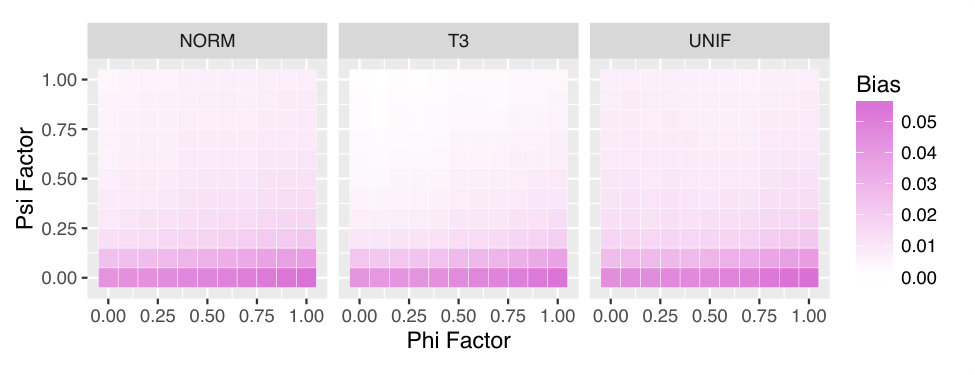 Figure 1
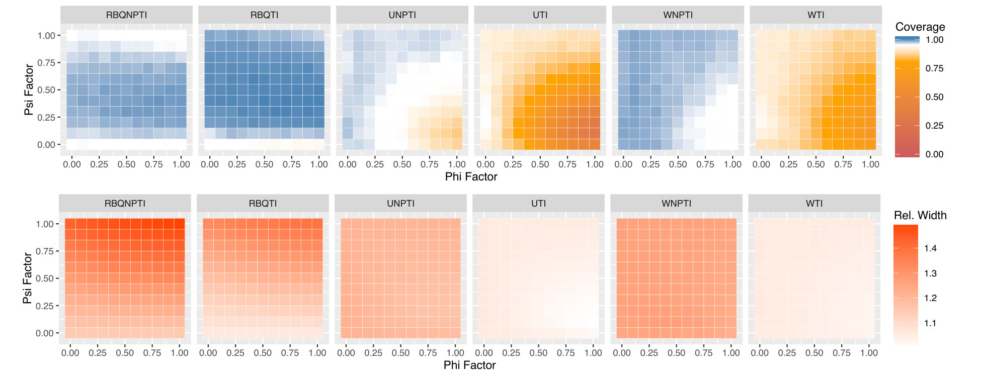 Figure 2
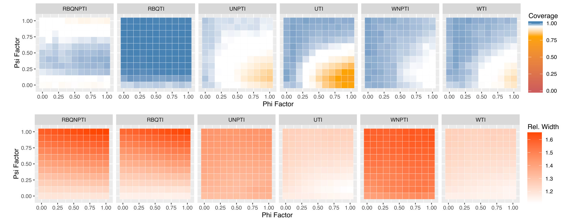 Figure 3
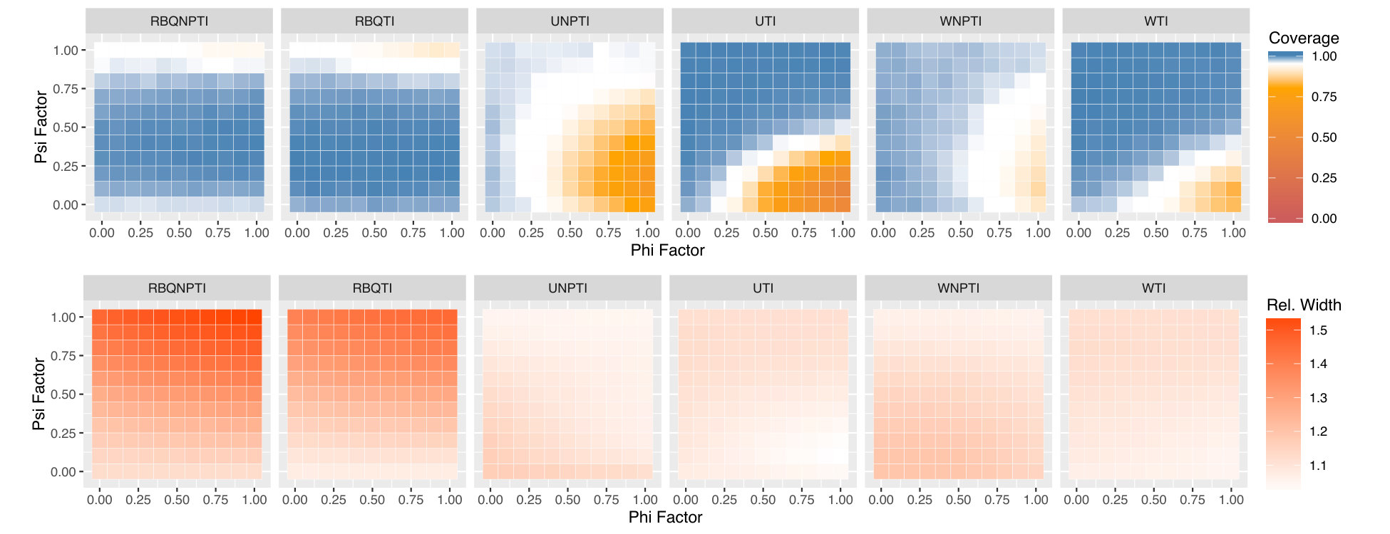 Figure 4
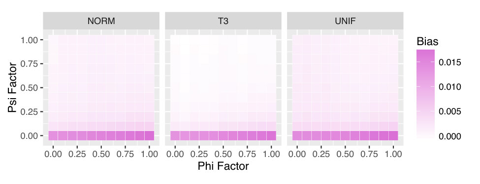 Figure 5
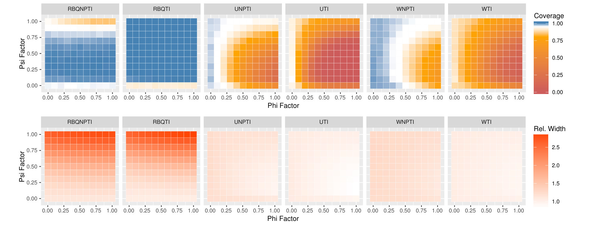 Figure 6
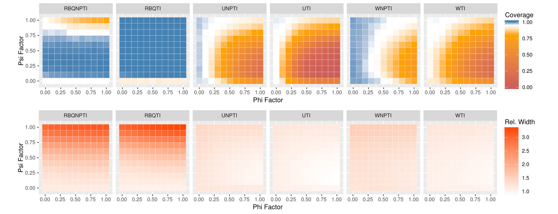 Figure 7
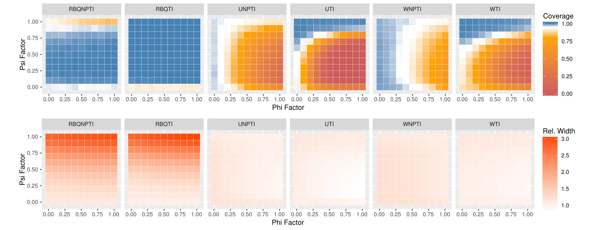 Figure 8
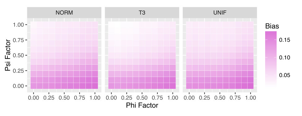 Figure 9
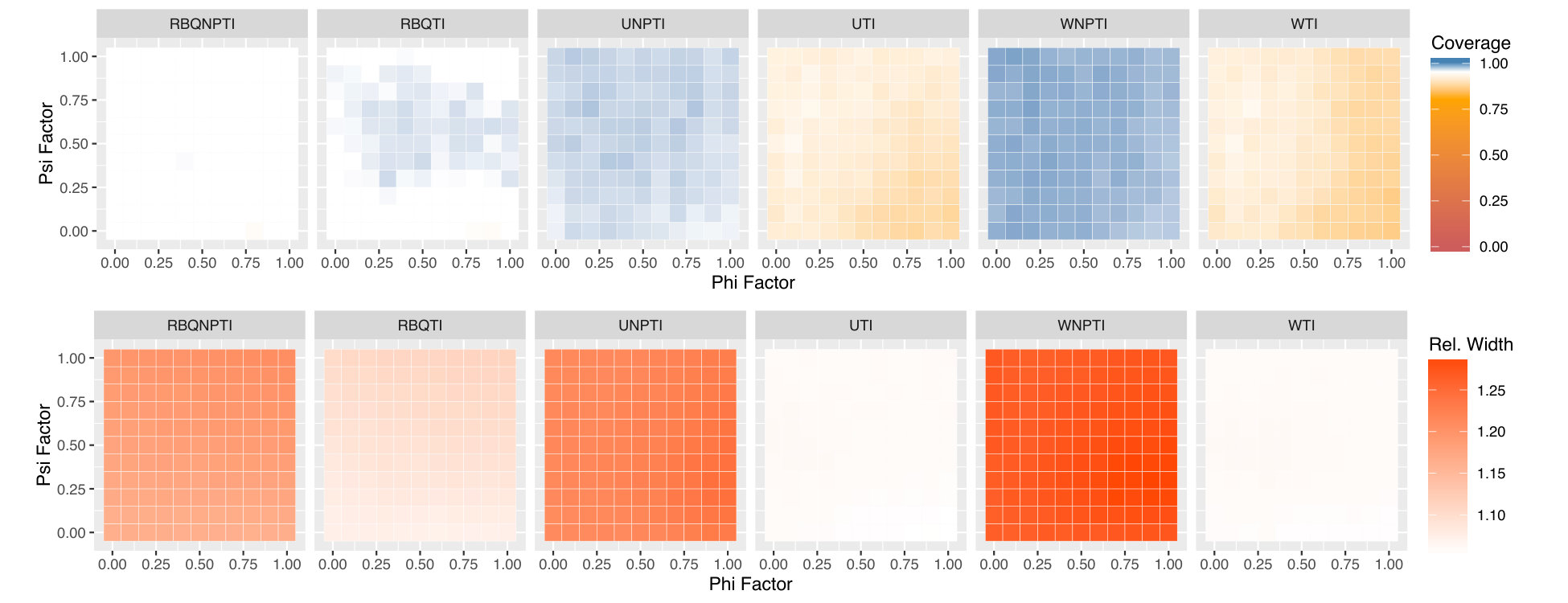 Figure 10
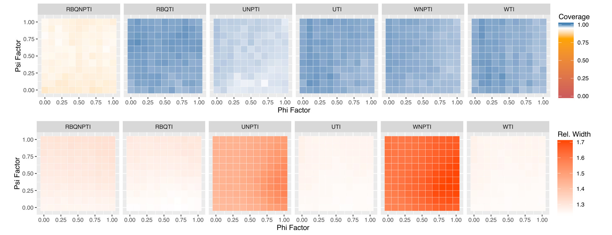 Figure 11
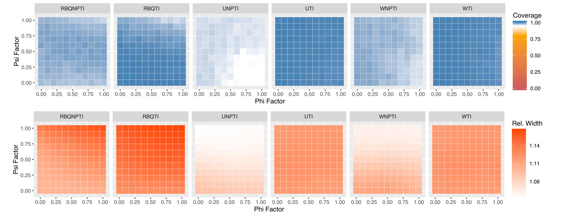 Figure 12
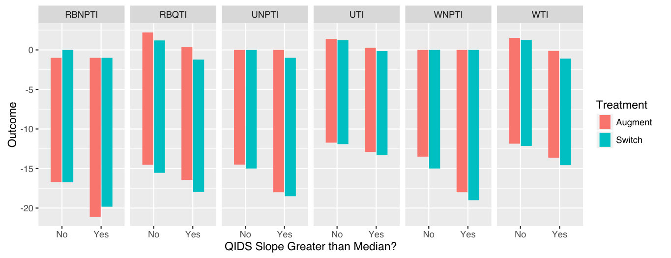 Figure 13
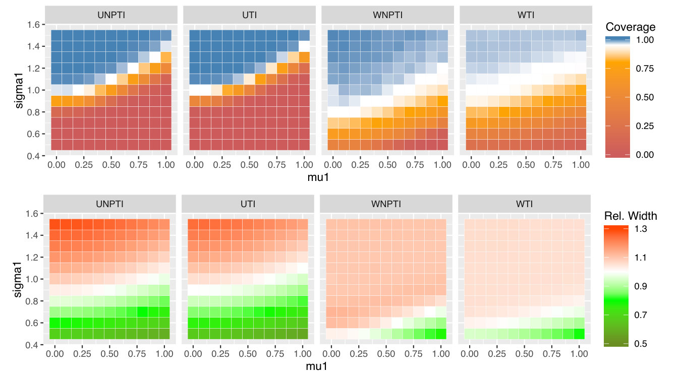 Figure 14
| RBQNPTI | Residual-Borrowing Non-parametric TI |
| RBQTI | Residual-Borrowing Normal-theory TI |
| UNPTI | Unweighted Non-parametric TI |
| UTI | Unweighted Normal-theory TI |
| WNPTI | Weighted Non-parametric TI |
| WTI | Weighted Normal-theory TI |
Peer Reviews
No public reviews on file for this paper yet. If you reviewed it on a platform where reviews are public (OpenReview, ICLR, NeurIPS, ICML), you can paste yours below so the community can read it here.
Videos
No videos yet. Explain this paper in a talk, walkthrough, or lecture? Add one.
On Prediction and Tolerance Intervals
for Dynamic Treatment Regimes
Daniel J. Lizotte
Departments of Computer Science and Epidemiology & Biostatistics,
The University of Western Ontario, London, Ontario, Canada
Arezoo Tahmasebi
Department of Epidemiology & Biostatistics,
The University of Western Ontario, London, Ontario, Canada
Abstract
We develop and evaluate tolerance interval methods for dynamic treatment regimes (DTRs) that can provide more detailed prognostic information to patients who will follow an estimated optimal regime. Although the problem of constructing confidence intervals for DTRs has been extensively studied, prediction and tolerance intervals have received little attention. We begin by reviewing in detail different interval estimation and prediction methods and then adapting them to the DTR setting. We illustrate some of the challenges associated with tolerance interval estimation stemming from the fact that we do not typically have data that were generated from the estimated optimal regime. We give an extensive empirical evaluation of the methods and discussed several practical aspects of method choice, and we present an example application using data from a clinical trial. Finally, we discuss future directions within this important emerging area of DTR research.
1 Introduction
Dynamic Treatment Regimes (DTRs), also known as adaptive treatment strategies or treatment policies, are a key tool for providing data-driven sequential decision-making support. A DTR is a sequence of decision functions that take up-to-date patient information as input and produce a recommended treatment. Thus, a DTR is a mathematical representation of the sequential decision-making process. Using this representation, we can use previously collected decision-making data to estimate an “optimal” DTR, where optimality is most often defined in terms of expected outcome. That is, a DTR is optimal if it produces the best outcome, on average, over a patient population. We will use this definition of optimality throughout our work.
Each decision in an optimal DTR is made in the service of achieving maximal expected outcome. However, the outcome of any particular individual under an optimal regime may vary widely from this expectation. Indeed, DTRs have been applied in many very challenging areas of medicine, including psychiatry, cancer, and HIV, where patient outcomes are known to be highly variable, or, equivalently from our perspective, difficult to predict.
It is with this variability in mind that we consider different methods for assessing the variability in individual outcomes under a given DTR. Our objective is to quantify for the decision-maker not our certainty about the expectation of outcomes, but rather our uncertainty about what the observed outcome might be for a particular patient.
We begin by formally defining DTRs, and we review point and interval estimation techniques for relevant parameters of the optimal DTR. We then review definitions and existing methods for confidence intervals, prediction intervals, and tolerance intervals. Following this background, we formally describe our problem of interest in the context of using DTRs to provide decision support.
We will see that the main technical challenge associated with constructing tolerance intervals for DTRs stems from not having a sample drawn from the correct distribution. Thus, our methods will use re-weighting and re-sampling to allow us to apply existing tolerance interval methods in this setting. To help illustrate the technical challenge, we first describe a naïve strategy for constructing tolerance intervals whose performance is poor, and we then present two novel strategies for constructing valid tolerance intervals for the response under a given dynamic treatment regime. We present an empirical evaluation of the methods, and we conclude by discussing their implications and directions for future work.
2 Background
In the following, we review basic concepts pertaining to DTRs, the estimation of optimal regimes, and concepts and issues surrounding interval estimation and prediction.
2.1 Dynamic Treatment Regimes
DTRs are a mathematical formalism meant to capture the decision-making cycle of information gathering, followed by treatment choice, followed by outcome evaluation. They have been defined at different levels of generality by many authors (Schulte et al., 2014; Laber et al., 2014b, a; Lizotte et al., 2012; Nahum-Shani et al., 2012a, b; Lizotte et al., 2010; Shortreed et al., 2011). Here, we focus on regimes with two decision points; thus for this work we consider a DTR to be a sequence of two functions which map up-to-date patient information at the first and second decision points, respectively, to distributions over the space of available treatments at each decision point. We represent the information (covariates) about a given patient at point by , which we view as a realization of a random variable . Similarly, we denote the chosen treatment (action) by , which is a realization of . For a patient who follows a DTR , we will have and . We let be the observed outcome or reward attained by a patient after following a regime, and we follow the convention that larger values of are preferable. For a patient following a given regime, we observe , the trajectory for that patient.
Trajectory data may come from various observational and experimental sources, for example from Sequential Multiple Assignment Randomized Trials (SMARTs) (Nahum-Shani et al., 2012a, b; Collins et al., 2014). A SMART is an experimental design under which patients follow a DTR that applies randomly assigned treatments. We will call such a DTR an exploration DTR or exploration policy. The goal of running a SMART is analogous to that of running a pragmatic randomized controlled trial—to evaluate the comparative effectiveness of different treatment options in an unbiased way. This comparative effectiveness information can then be used to estimate an optimal DTR. An optimal DTR is a pair of decision functions that maximize where . Thus, an optimal DTR produces maximal expected outcome when applied to a population of patients. In this work, we focus on the setting where the exploration DTR is stochastic, but the candidate optimal DTRs under consideration are deterministic.
2.2 -learning
Several methods are available for estimating an optimal DTR from data collected under an exploration DTR. Here, we review one such method called -learning (Schulte et al., 2014; Huang et al., 2015). -learning works by estimating functions ( for “quality”) that predict expected outcome given current covariates and treatment choice. In our 2-decision point setting, we have
[TABLE]
Note that unlike the expectation in the previous section which averages over patients, gives the expectation of conditioned on particular patient observations and treatment choices. The definition of implies an optimal decision function . can be estimated using any regression method. Having obtained an estimate of , our estimate of the optimal second decision function is .
The optimal -function for the first decision point produces the conditional mean of given and and given that the optimal decision function is used at the second decision point. In -learning, we estimate by
[TABLE]
where the expectation is over conditioned on and . The quantity is sometimes called the pseudooutcome, and is denoted . In order to estimate , we compute the pseudooutcome for each trajectory in our dataset, and then regress them on and to estimate . Again, any regression method can be used to estimate , in principle. Our corresponding estimate of the optimal first decision function is then , and our estimate of the optimal DTR is . Note that this DTR is deterministic.
We focus on -learning in this work, but several other methods are available for estimating optimal DTRs, including -learning (Blatt et al., 2004; Schulte et al., 2014), the closely-related -estimation (Moodie, 2009; Orellana et al., 2010; Barrett et al., 2014), and direct policy search (Zhao and Laber, 2014; Zhao et al., 2015).
2.3 Interval Estimation
For consistency, in the following we use s to represent observed outcomes, and s to represent covariates, even in non-regression settings.
2.3.1 Confidence Intervals
A confidence interval with level for a parameter is a functional of a dataset of realizations of a random variable , with the property that
[TABLE]
The probability statement (1) is over datasets containing i.i.d. samples of . The goal of a confidence interval is to provide confidence information about the estimated location of an underlying distributional parameter. Though not our main focus, confidence intervals are by far the most well-known class of interval estimates, and they are closely related to the prediction and tolerance intervals we will develop and investigate.
2.3.2 Prediction Intervals
A prediction interval with level is a functional of a dataset of realizations of a random variable , with the property that
[TABLE]
Here, represents a single future observation that was not contained in the original data . The goal of a prediction interval is to provide confidence information about where this new observation might fall. However, we note, as others have (Vardeman, 1992), that there is often confusion surrounding the probability statement (2). In particular, the statement is over the joint distribution of . A prediction interval formed from a dataset traps one additional observation with probability . It offers no guarantees about trapping more than one additional observation, and indeed no guarantees regarding our confidence in the content of an interval, that is, of the quantity where is the cumulative distribution function of . (For example, a prediction interval that has content half the time and content half the time has property (2) for , as does an interval that always has content .)
The well-known normal-theory prediction interval for (Neter, John and Wasserman, William and Kutner, 1989) is given by
[TABLE]
where is the sample mean, the sample standard deviation, and is the quantile of a -distribution with degrees of freedom. Note that the validity of (3) is predicated on normality of , regardless of sample size.
The corresponding prediction interval for in the linear regression setting on parameters is
[TABLE]
where represents the location of a new sample, is the prediction of , is the sample standard deviation of the residuals, is the design matrix for the regression, and is the quantile of a -distribution with degrees of freedom. Equation (4) is predicated on the normality of and on homoscedasticity of the residuals.
2.3.3 Tolerance Intervals
A tolerance interval with level and content is also a functional of a dataset . It has the property that
[TABLE]
where is the cumulative distribution function of . Thus, a tolerance interval formed from a dataset traps at least of the probability content of with probability , where the probability is over datasets.
One well-known normal theory approximate tolerance interval for with confidence and content is given by Krishnamoorthy, Kalimuthu and Mathew (2009) as
[TABLE]
where is the sample mean, is the quantile of a non-central distribution with 1 degree of freedom and noncentrality parameter , and is the quantile of a with degrees of freedom.
The corresponding tolerance interval for in the linear regression setting on parameters is (Young, 2013)
[TABLE]
where is the prediction of , is the sample standard deviation of the residuals, is Wallis’ “effective number of observations” (1951), and is the standard error of . Again, validity of (6) and (7) is predicated on the normality of and , respectively; (7) is also predicated on homoscedasticity.
Wilks (1941) proposed a non-parametric tolerance interval that assumes only continuity of . The interval is given by the sample values corresponding to the minimum and maximum ranks for which
[TABLE]
where is the beta cumulative distribution function. Thus, the interval is constructed simply by truncating the sample to the ranks satisfying (8), and then taking the minimum and maximum of the truncated sample to be the lower and upper limits of the tolerance interval, respectively.
3 DTRs for Decision Support
DTRs are an ideal formalism for providing data-driven decision support. The most basic approach to providing decision support would be to estimate an optimal DTR from SMART data, and then provide the estimated DTR to a decision maker, perhaps as a computer-based tool that produces the estimated optimal treatment by using current patient information as input to the previously estimated DTR.
Early in the development of DTRs it was recognized that this approach is problematic because it provides no confidence information about our recommendations. Just as we would not recommend one treatment over another if no statistically significant difference were obtained from a standard randomized controlled trial (RCT), neither should we recommend a single treatment in a DTR if in fact the alternatives are not known to be inferior with high confidence. This led to the development of confidence interval methods for the difference in mean expected outcome under different treatment choices within a regime (Chakraborty et al., 2010, 2013; Chakraborty and Moodie, 2013; Laber et al., 2014b; Chakraborty et al., 2014).
Such intervals can give us confidence that if we do recommend a single treatment, that treatment will provide a better outcome, in expectation over patients. However, they do not provide any information about what the range of possible outcomes might actually be for an individual patient. In particular, large SMARTs with 100s to 1000s of patients may discover statistically significant differences in mean outcome even when the effect sizes are small to moderate and variance in outcomes is still substantial. If this is the case, it may be better to avoid recommending a single treatment, or at least to provide more nuanced information about what the patient’s experience is likely to be under the different treatment options.
In this work, we consider tolerance intervals as one method for providing this information. For a patient with at the first decision point, rather than recommending treatment (even if it is statistically significantly better than the alternative in terms of mean outcome) we would present tolerance intervals for the outcome under each possible action, and allow the decision-maker (or the patient-clinician dyad, in the context of patient-centred care (Barry and Edgman-Levitan, 2012)) to decide on treatment based on the range of probable outcomes indicated by the intervals. For each interval, we condition on the observed , the hypothetical , and the estimated optimal regime for the second stage.
Thus, we will construct tolerance intervals for , marginal over (whose distribution is governed by and ) and (whose distribution is governed by , , and .) To do so, we will adapt several standard methods because typically we do not have observations drawn from this distribution. This is because, as we noted above, data from SMART studies and similar sources are generated according to an exploration DTR , rather than according to an estimated optimal DTR .
3.1 Aside: Non-regularity
It is well-known that many kinds of inference on the parameters of an estimated optimal dynamic treatment regime, including confidence intervals, are plagued by issues of non-regularity (Laber et al., 2014b). Briefly, non-regularity is a result of the sampling distributions of corresponding estimators changing abruptly as a function of the true underlying parameters. It can lead to bias in estimates and anti-conservatism in inference. In dynamic treatment regimes, non-regularity occurs and inference is problematic when two or more treatments produce (nearly) the same mean optimal outcome. In this work, we will not specifically develop methods that are robust to non-regularity. This is because even in the absence of non-regularity, i.e. when optimal values are well-separated from sub-optimal ones, there is significant variability in the performance of “standard” tolerance interval methods that is worthy of exploration and analysis. We will return to this point in the Discussion.
4 Methods
We now detail our strategies for constructing tolerance intervals for . As we mentioned above, the fundamental challenge of constructing intervals for this quantity is that in general we do not have samples drawn from this distribution—otherwise, we could use off-the-shelf tolerance interval methods. Note that we can use off-the-shelf methods for tolerance intervals for , because there is no need to account for future decision-making in that case; thus our work focuses on the first decision point. We begin by presenting a naïve approach to constructing tolerance intervals that helps illustrate the main technical challenge to be addressed, and then we present our two proposed strategies: inverse probability weighting, and residual borrowing.
4.1 Naïve -Learning Tolerance Intervals
Standard -learning involves estimating , which predicts the expected under the optimal regime. However, it does so using the pseudooutcome as the regression target, rather than the observed . Since the pseudooutcome targets are themselves predicted conditional means of , they carry no variance information about under the estimated optimal policy, even among trajectories that (by chance) followed the estimated optimal policy. To see this, suppose that we had several trajectories, all of which had the same , and all of whom happened to follow the estimated optimal policy. Even though their observed outcomes might have all been different, simply due to unexplained (but still important) variation in , they would all be assigned the same pseudooutcome value, and the sample variance of the pseudooutcomes in this group is zero.
This observation highlights the key aspect of -learning and related methods that precludes direct estimation of variability in . Dynamic programming methods for estimating conditional means of sequential outcomes can “throw away” residual variance without negative repercussions when backing up values, essentially because of the law of total expectation. The benefit of this approach is a reduction in the variance of estimates by allowing the use of the entire dataset of trajectories for estimating -functions for earlier decision points. The drawback is that such methods cannot directly estimate other distributional properties of , including variance and higher-order moments, quantiles, and so on.
If most of the variability in were explained by and —that is, if the variance of were nearly zero—we might be able to construct approximate tolerance intervals for by constructing parametric tolerance intervals for the pseudooutcome, for example using (7). In the case of a saturated model with discrete and , we could construct non-parametric tolerance intervals for each pattern of using the pseudooutcome with (8). However, as expected, will see in our empirical results that this approach is not very effective if in fact the variance of is not near zero.
4.2 Inverse Probability Weighting
One approach to obtaining variance information about under is to select from our dataset only those trajectories whose second-stage treatment matches what would have assigned, i.e., the trajectories for which . This subset contains all of the trajectories that have positive probability under the estimated DTR.
Consider a joint distribution over conditioned on and . (All statements in the remainder of this subsection are implicitly conditioned on and ; explicitly maintaining this is too cumbersome.) Here, is the action chosen by , and is the action chosen by , which is assumed to be deterministic given . Let (for match111Note we are not matching trajectories with other trajectories—we are identifying trajectories whose action matches a DTR of interest.) be if , or [math] otherwise. Let be binary, and define such that if and if . The dependencies among all of these variables are illustrated in Figure 1 using a directed graphical model (Koller and Friedman, 2009).
The distribution of among matched trajectories is governed by . The distribution of among trajectories gathered using is . Note that while the distribution of is identical to the distribution of due to the conditional independence structure, the distribution of may be different from if there is dependence of on . We describe this phenomenon using the following lemma.
Lemma 1**.**
Let be defined as above, and assume . Then
[TABLE]
Proof.
In the following, we abuse notation by allowing to represent a probability or a density, as appropriate, and we allow to indicate a sum or an integral. The message in any case remains the same.
First we note that
[TABLE]
The data generating distribution under is
[TABLE]
where the last step follows from conditional independence of and given and . Furthermore,
[TABLE]
where the second step follows because is deterministic given 222This assumption is critical: if is not deterministic, the relationship between and is more complicated. and from the definition of and , and the third step follows from independence of and . By combining (10) and (11) and comparing with (9), we obtain
[TABLE]
where the final step is by independence of and . ∎
Corollary 1**.**
If and are independent, then has the same distribution as .
Proof.
Follows immediately from Lemma 1. ∎
To achieve independence of and , we could ensure during data collection that is independent of , which in turn can be achieved by equal randomization independent of . This is common, but not universal, in SMART designs (Collins et al., 2014). If and , then
[TABLE]
Hence, if , then , and . Using this subset of trajectories whose matches , we can regress on and to construct tolerance intervals using (7), or, as above, we can construct non-parametric tolerance intervals for each pattern of using (8).
Dependence of on is problematic because of the effect of on . When depends on , conditioning on can affect the distribution of through , meaning that the distribution of we estimate by collecting data under is not what we would have obtained had we collected data under and ignored (i.e. marginalized over) .
To correct the problem of the distribution of among the matched trajectories, we employ inverse probability weighting. To do so, we construct a propensity score model, not for the probability of treatment, but for the probability of following the estimated optimal DTR, i.e. . Using this model, we can then re-weight the trajectories so that the distribution of matches the distribution of as well as possible. The weight function is therefore
[TABLE]
These are sometimes known as importance weights. We note that in causal inference, importance weights are sometimes used to adjust for an association between the probability of receiving treatment and the observed outcome. Here, they are used to adjust for an association between the probability of following the estimated optimal policy and the observed outcome through the variable . Note that estimating the two densities in (12) separately is not necessary to estimate the function ; it can be estimated using any density ratio estimation method. Logistic regression is one common approach but many others are available. In related weighting methods for causal inference, practitioners have found that a flexible model for is often preferable to a simpler one (Ghosh, 2011).
To use the weighted data for building tolerance intervals, we must adapt existing methods for use with the weights. To build normal-theory regression tolerance intervals using the weighted data, we first estimate using weighted least squares. We then use the resulting mean estimate, together with a weight-based sandwich estimate of to construct the tolerance interval as per (7). To build non-parametric tolerance intervals, we obtain weighted estimates of the ranks obtained by linear interpolation of the weighted empirical distribution (Harrell et al., 2015). We then construct the Wilks interval as per (8).
Figure 2 shows the empirical results of applying weighted tolerance intervals in a simple scenario. Our goal here is to verify that the weighting scheme can counteract some of the dependence on . (We will evaluate them more fully in the next section.) The data are drawn from a two-variable generative model with and . Our goal is to produce a tolerance interval for , marginal over , using only data for which . The sample size for was , and the weights were computed analytically. Parameters for were fixed at and . Parameters for were varied to illustrate how performance of the weighted tolerance intervals changed as the distribution of deviated from the marginal distribution of . The top row of heatmaps shows the coverage of each method, that is, the proportion of times out of 1000 Monte Carlo replicates for which the computed tolerance interval had at least probability content. The confidence level was set to ; in the plot, Monte Carlo coverages that are not statistically significantly different from 0.95 are coloured pure white. Over-coverage is coloured blue, and under-coverage is coloured orange. The second row plots the average width of the tolerance intervals, normalized by the width of the optimal tolerance interval constructed from the true quantiles of , with unit relative width coloured white.
Methods beginning with U are unweighted, and methods beginning with W are weighted. Methods containing NP are nonparametric, and those without NP are normal-theory. (Table 1 gives the complete key to the method names.) Note that except when and , is nonnormal. As one would expect, performance when is very good across all methods; in this case, , and weighting is not needed. When is near zero and/or is larger than , most of the mass of overlaps the mass of , and all intervals tend to over-cover. This is indicated by the blue regions in the upper-left corner of the coverage plots, and is larger in the weighed methods than the unweighted methods. Conversely, when does adequately overlap the mass of because is farther from [math] and/or is less than , we see undercoverage indicated by the orange in the lower-right of the plots. Again, this is mitigated by weighting. The non-parametric methods provide better coverage than the normal-theory methods; this is not surprising since is not normal in most cases. The width plots verify that the weighted methods bring the extreme widths observed from the unweighted methods closer to optimal.
This example verifies that the weighted methods we propose can substantially reduce over- and under-coverage in cases where there is mismatch between the observed distribution and the distribution of interest. However, they cannot eliminate it entirely when the distributions of and are very different. This is to be expected; estimating say the mean of one distribution using an importance-weighted sample is challenging in practice. Estimating the tails of that distribution is even more challenging. Nonetheless, there is value in the weighted approach, and we will explore it further in the DTR setting in the next section.
4.3 Residual Borrowing
We now present a different approach to ensuring that our analysis captures the joint distribution correctly, and hence captures variability in correctly when we marginalize over . To do so, we return to the -learning approach, which estimates using regression. As discussed above, the pseudooutcome for each trajectory represents our best estimate of when . This estimate is available for all trajectories in our dataset, including those for which . Rather than naïvely constructing tolerance intervals based on the regression of on and , we create a new pseudooutcome for each point: For trajectories with , we set . For trajectories with , we set , where , and is an estimate of the distribution of the residuals among trajectories with . We call this procedure residual borrowing. We then construct tolerance intervals using the regression of on and .
Unlike the , the retain information about the distribution of . Furthermore, since we use all of the trajectories in our original dataset, our empirical distribution of is representative of the true generative model. The distribution could be the empirical distribution of the appropriate residuals, or it could be a smoothed estimate, e.g., a kernel density estimate. In our simulations, we found that a smoothed estimate works better than sampling from the empirical distribution.
5 Empirical Results
We now present results of six tolerance interval methods, which are listed in Table 1, using a simulation study. Our goals are to: 1. verify that inverse probability weighted methods can succeed where the unweighted methods fail, and test their limits; and, 2. to assess the difference in performance between the inverse probability weighted methods and the residual borrowing methods. Note that we do not include results from the naïve method as it performs very poorly.
The generative model from the study is taken from Schulte et al. (2014), with modifications. We begin by reviewing that model and discussing our modifications to it; we then present and discuss the performance of our methods.
5.1 Generative Model
The generative model has decision points. is binary, is binary, is continuous, is binary, and is continuous. The generative model under the exploration DTR is given by
[TABLE]
Here, . The original model is indexed by
[TABLE]
to which we have added four parameters: is a factor multiplying , its default is 1; is a factor multiplying , its default is 1; gives the conditional distribution of with given mean and variance; its default is the normal distribution and the default is 10. We have emphasized these parameters by displaying them in boxes.
Our parameter allows us to control the degree to which state information influences treatment selection under the exploration (data-gathering) DTR. For , we have the original exploration used by Schulte et al., and for , we have uniform randomization over treatments independent of state and previous treatment. allows us to control the effect of treatment on . For we have the treatment effect specified by Schulte et al., and for we have no treatment effect at the second stage. allows us to control the shape of the error distribution to see its effect on the tolerance interval methods; Schulte et al. used a normal error, but we will explore heavier and lighter-tailed errors while holding variance constant.
This family of generative models allows us to explore what happens to the performance of tolerance interval methods when we have dependence of on during the generating process. While most of the SMART studies we are aware of use a simple randomization strategy where the distribution of does not depend on (which is the case here when e.g. , giving a simple 50:50 randomization strategy), we expect that more studies akin to “adaptive trials” with state-dependent randomization will become attractive in the future.
Based on the function333Denoted by Schulte et al. which determines the expected value of , we can immediately see that the optimal second stage decision function is
[TABLE]
5.2 Working Model
Our working model for is
[TABLE]
Having computed least squares estimates and , our estimate of the optimal second-stage decision function is
[TABLE]
and the pseudooutcome for the th trajectory is
[TABLE]
Our working model for is the saturated model
[TABLE]
Having computed least squares estimates and by regressing the pseudooutcomes on and , our estimate of the optimal first-stage decision function would be444Schulte et al. (2014) give the true optimal values of and as a function of the other model parameters.
[TABLE]
5.3 Tolerance Intervals
In many studies of DTR methods, the focus is on point and interval estimates of the optimal stage 1 decision parameters (Chakraborty et al., 2010, 2013; Chakraborty and Moodie, 2013; Laber et al., 2014b; Chakraborty et al., 2014). In this work, we will investigate methods for constructing tolerance intervals for
[TABLE]
Note that our goal is to construct tolerance intervals for under the estimated optimal regime rather than under the optimal regime. The reason for this is pragmatic: we assume that it is the estimated optimal regime that would be deployed in future to support decision-making.
We begin by estimating using the working models (13,14). We then compute the pseudooutcome for each trajectory, and the match indicator .
5.3.1 Unweighted Methods
To construct the unweighted normal-theory TIs, we regress on and according to working model (15) but using only trajectories with . We then apply (7) to construct the four tolerance intervals.
To construct the unweighted nonparametric TIs, we divide the trajectories with into four mutually exclusive groups according to their values. We then construct the four tolerance intervals by applying the Wilks method (8) to each group.
5.3.2 Weighted Methods
To construct the weights, we first form kernel density estimates for and for . The weight for a trajectory with index that has is then given by
[TABLE]
While logistic regression might be viewed as a more obvious choice for this task, we found that its attendant monotonicity assumptions were often violated, and that the pair of kernel density estimates were the simplest way to produce a more flexible model in this low-dimensional setting.
To construct the weighted normal-theory TIs, as above we compute a weighted regression of on and according to working model (15) but using only trajectories with . We then apply (7) to construct the four tolerance intervals; in this case, we use the sandwich estimate (Huber, 1967; White, 1980) with the weights to compute . This makes the method somewhat more robust.
To construct the unweighted nonparametric TIs, we divide the trajectories with into four mutually exclusive groups according to their values. We then construct the four tolerance intervals by applying our weighted modification of the Wilks method (8) to each group.
5.3.3 Residual Borrowing
For the residual borrowing methods, within each group, we first form a kernel density estimate using the residuals among the trajectories with . We then set for each trajectory with , and sample from the kernel density estimate for trajectories with . We then either regress using the working models to create the regression tolerance intervals, or we again divide up the data according to and to construct non-parametric tolerance intervals.
5.4 Results
Using the foregoing generative model, working models, and tolerance interval methods, we ran a suite of simulations to investigate performance. Experiments varied by , and , for a total of different experimental settings. Both and were varied from [math] to in increments, and took values in . We examined settings with as normal, uniform, and with 3 degrees of freedom, each scaled to have the appropriate . For each setting, we drew 1000 simulated datasets each of size , computed tolerance intervals using each of the six methods, and evaluated their content, that is, what proportion of was captured by each interval, and their relative width, given by , where is the width of the optimal tolerance interval computed using the and quantiles of the true distribution. For all experiments, we set and . All kernel density estimates were one-dimensional, and used the default optimal bandwidth. All experimental code was written in R (R Core Team, 2015), and is publicly available.
Figures 5, 6, and 7 display the results of all of our experiments as heatmaps using the same approach as Figure 2. Monte Carlo coverages that are not statistically significantly different from 0.95 are coloured pure white, Over-coverage is coloured blue, and under-coverage is coloured orange. The second row of each subplot gives the average width of the tolerance intervals.
Figure 5(a) contains the original model setting proposed by Schulte et al. (2014) in the upper-right corners of its heatmaps. In this setting, the weighted and unweighted normal-theory tolerance intervals undercover slightly, while the weighted and unweighted non-parametric methods overcover, and are much wider. The residual-borrowing methods perform best in this setting, with the normal-theory residual-borrowing intervals achieving near-nominal coverage with modest width. There is relatively little variation in coverage and width across and in this setting, we believe because the noise level is quite high relative to the effect of even when . In Figure 5(b), was chosen to be a -distribution with 3 degrees of freedom, scaled to have variance and shifted by . In this heavy-tailed setting, it is the non-parametric residual-borrowing method that slightly undercovers, while the other methods overcover somewhat. As in the normal case, the weighted and unweighted nonparametric methods are very wide. Figure 5(c) uses a scaled and shifted uniform distribution for , again maintaining . In this light-tailed setting, in contrast to Figure 5(b), it is the normal-theory intervals which tend to be wide, while the non-parametric ones are narrower. The residual-borrowing intervals are wide as well. All intervals achieve nominal or greater coverage in this setting.
We see a striking change as we examine the lower-noise settings in Figure 6, which have . Here, we start to see dependence of performance on and . As in Figure 5(a), in Figure 6(a) we see the normal theory intervals undercovering, although we now see a definite trend that worsens as increases, and as decreases. We also see this trend among the non-parametric methods, which range from overcovering to undercovering as we move across and . Overall, we see the greatest coverage when the effect of is quite strong (topmost rows), or if the dependence of on is weak (leftmost rows.) As we discussed earlier, when (leftmost columns) there is no dependence of on , and thus weighting is unnecessary. Furthermore, we not only obtain a uniform probability of across , but also a uniform probability of across . This uniformity likely leads to improved estimates of , and in turn to better coverage of the tolerance intervals. The decrease in performance for low may be due to non-regularity: when , there is in fact no effect of on . However, assuming continuity of the appropriate distributions, our estimated will be nonzero almost always, and our plug-in estimate of the value of will be positive almost always. Defining , the empirical bias in the value of is
[TABLE]
Figure 3 shows the average empirical bias in our estimate of the average value of using , as a function of and . We can see that the bias is concentrated at the bottom of the plots, near . This is precisely where there is more than one nearly-optimal action and non-regularity is known to be a problem.
We see the problems worsen in Figure 7, where we set . We hypothesise that this is because proportionately even more of the variability in is attributable to variability in , and accurate estimation of becomes that much more important. All of the matched subset methods have severe undercoverage for large values of and low values of . Weighted methods mitigate this. The residual-borrowing methods achieve much better coverage, but at the cost of much wider intervals.
5.5 Discussion
Based on our simulation study experiments, we believe that designing the exploration DTR to have uniform randomization over actions is highly beneficial for estimating tolerance intervals. When this is the case, all methods gave reasonable results in almost all scenarios. Some knowledge of the error distribution may help choose a method that will result in reasonable widths. If uniform exploration is not possible, the residual-borrowing methods appear to be the most robust to undercoverage, followed by the weighted methods, followed by the unweighted methods. That said, it would be prudent to perform a simulation study under a scenario “close” to the analysis at hand if possible; to facilitate this we have released our R code (R Core Team, 2015) so that researchers and practitioners can explore other scenarios.
6 Example: STAR*D
We present an example of the application of the TI methods we have described to real-world clinical trial data. The Sequenced Treatment Alternatives to Relieve Depression (STAR*D) study followed an initial population of 4041 patients as they were treated using different antidepressant medications and cognitive behavioural therapy (Rush et al., 2004). There were a total of three decision points at which randomisation took place, with different treatment options available at each one. Outcomes were measured using the clinician-rated Quick Inventory of Depressive Symptomatology (Rush et al., 2003). We will examine two such decision points corresponding to Level 2 and Level 3 of the study, which will correspond to the first and second decision points in our analysis.
We construct tolerance intervals for STAR*D at Level 2 (our decision point 1), having estimated a function and estimated optimal policy for Level 3 (our decision point 2.) We use exactly the same -learning working model and estimation procedure as Schulte et al. (2014) to develop and the pseudooutcomes; we refer the interested reader to their work for more details. In summary, the state variables we use are up-to-date QIDS measures of patient symptoms, and the outcomes we use are based on later QIDS measurements that have been negated so that higher values are preferable. At decision point 1, we elect to use a binary state variable indicating whether the previous slope in QIDS score for a patient is greater than the median. Higher QIDS scores indicate worse symptom levels, so this state variable effectively identifies patients whose disease status is worsening most quickly. At both decision points, the treatment choice is whether to “augment” the current medication with another, or to “switch” to another medication altogether.
We applied the six TI methods described previously to the data, using the choice to switch or augment treatment as , and letting be an indicator variable for QIDS slope being greater than the median slope. We see that generally the intervals are quite wide, and that there is severe overlap of TIs for different treatments. This reflects the high variance and low treatment effect we observe in this data. However, the intervals do capture prognostic information: the intervals for (indicating severely worsening symptoms) are wider, with a decreased lower bound indicating that such patients may have poorer outcomes relative to those with more stable symptoms prior to the decision point. The maximum attainable outcome in this problem is [math], since QIDS cannot go below [math]. We note that the parametric TI methods can produce upper bounds greater than [math] and lower bounds that appear to be a bit optimistic. Hence, we suggest that one of the non-parametric methods would be a sensible choice for STAR*D.
7 Conclusion
We have developed and evaluated tolerance interval methods for dynamic treatment regimes that can provide more detailed prognostic information to patients who will follow an estimated optimal regime. We began by reviewing in detail different interval estimation and prediction methods and then adapting them to the DTR setting. We illustrated some of the challenges associated with tolerance interval estimation stemming from the fact that we do not typically have data that were generated from the estimated optimal regime. We gave an extensive empirical evaluation of the methods and discussed several practical aspects of method choice. We demonstrated the methods using data from a pragmatic clinical trial. We now take the opportunity to discuss future directions of research on tolerance intervals for dynamic treatment regimes.
7.1 Future Directions
Our work lays the foundation for extending tolerance interval methods for dynamic treatment regimes in several different directions.
The normal theory TI methods we employed used an estimate of the residual distribution that is pooled over and . The non-parametric methods estimated the residual distributions separately for the different discrete . A compromise solution that partially shares residual information across different configurations of , perhaps in a data-driven, adaptive fashion, may provide improved performance and wider applicability. (Note that the non-parametric methods we described are not applicable if is continuous.)
We have treated DTRs with two decision points, but in general we would like to have tolerance intervals for multiple decision points. Such methods would potentially have to address uncertainty stemming from “parameter sharing,” across time points. It is known (Chakraborty et al., 2016) that the effects of model misspecification and non-regularity can compound in the multiple decision point setting, and the impact of this on tolerance intervals is not yet known.
While we assumed a single outcome measure throughout our work, several methods have been described for estimating DTRs in the presence of multiple outcomes (Lizotte et al., 2012; Laber et al., 2014a; Lizotte and Laber, 2015). Joint tolerance intervals/tolerance regions for this setting would be equally important as they are in the standard, single-outcome setting.
We observed some problems associated with biased estimates of the value of the estimated policy, which is caused by non-regularity. The problem of non-regularity in optimal DTR estimation has been addressed in the confidence interval setting using different approaches, including pre-testing (Laber et al., 2014b) and shrinkage (Chakraborty et al., 2010, 2013). We have not explicitly incorporated either of these ideas in the methods we presented; doing so may lead to methods that are more robust to small or zero treatment effects at the second stage yet do not pay a high cost in terms of width.
Fernholz and Gillespie (2001) have presented a method to re-calibrate tolerance intervals using the bootstrap. They propose a bootstrap method to estimate the content of a given tolerance interval—first they construct a tolerance interval with nominal (or “requested”) content , but then they use the bootstrap to estimate what the actual content. This could potentially be used to identify when tolerance methods fail on dynamic treatment regimes, or they may be used simply to give more accurate confidence information to the decision maker. For example, we may attempt to construct a tolerance interval for , but if it turns out that the actual content is , the interval may still be useful if the decision-maker is made aware of this fact. Future work to adapt the calibration procedure could prove promising.
Finally, a Bayesian approach to the predictive estimation problem may prove fruitful in some settings. Saarela et al. (2015) have laid groundwork for this direction of research.
Acknowledgements
This work was supported by the Natural Sciences and Engineering Research Council of Canada. Data used in the preparation of this article were obtained from the limited access datasets distributed from the NIH-supported “Sequenced Treatment Alternatives to Relieve Depression” (STARD). STARD focused on non-psychotic major depressive disorder in adults seen in outpatient settings. The primary purpose of this research study was to determine which treatments work best if the first treatment with medication does not produce an acceptable response. The study was supported by NIMH Contract #N01MH90003 to the University of Texas Southwestern Medical Center. The ClinicalTrials.gov identifier is NCT00021528.
The reference list from the paper itself. Each links out to its DOI / PubMed record.
- 1Barrett et al. [2014] Jessica K. Barrett, Robin Henderson, and Susanne Rosthøj. Doubly Robust Estimation of Optimal Dynamic Treatment Regimes. Statistics in Biosciences , 6(2):244–260, nov 2014. ISSN 1867-1764. doi: 10.1007/s 12561-013-9097-6 .
- 2Barry and Edgman-Levitan [2012] Michael J. Barry and Susan Edgman-Levitan. Shared decision making â the pinnacle of patient-centered care. New England Journal of Medicine , 366(9):780–781, 2012. doi: 10.1056/NEJ Mp 1109283 .
- 3Blatt et al. [2004] D. Blatt, S.A. Murphy, and J. Zhu. A-learning for approximate planning. Technical Report 04-63, The Methodology Center, The Pennsylvania State University, University Park, PA, 2004.
- 4Chakraborty and Moodie [2013] Bibhas Chakraborty and Erica E.M. Moodie. Statistical Methods for Dynamic Treatment Regimes . Statistics for Biology and Health. Springer New York, New York, NY, 2013. ISBN 978-1-4614-7427-2. doi: 10.1007/978-1-4614-7428-9 .
- 5Chakraborty et al. [2010] Bibhas Chakraborty, Susan Murphy, and Victor Strecher. Inference for non-regular parameters in optimal dynamic treatment regimes. Statistical Methods in Medical Research , 19(3):317–343, jun 2010. ISSN 0962-2802. doi: 10.1177/0962280209105013 .
- 6Chakraborty et al. [2013] Bibhas Chakraborty, Eric B. Laber, and Yingqi Zhao. Inference for Optimal Dynamic Treatment Regimes Using an Adaptive m -Out-of- n Bootstrap Scheme. Biometrics , 69(3):714–723, sep 2013. ISSN 0006341 X. doi: 10.1111/biom.12052 .
- 7Chakraborty et al. [2014] Bibhas Chakraborty, Eric B Laber, and Y.-Q. Zhao. Inference about the expected performance of a data-driven dynamic treatment regime. Clinical Trials , 11(4):408–417, aug 2014. ISSN 1740-7745. doi: 10.1177/1740774514537727 .
- 8Chakraborty et al. [2016] Bibhas Chakraborty, Palash Ghosh, Erica E. M. Moodie, and A. John Rush. Estimating optimal shared-parameter dynamic regimens with application to a multistage depression clinical trial. Biometrics , page Epub ahead of print, 2016. ISSN 1541-0420. doi: 10.1111/biom.12493 .