Trend and Variable-Phase Seasonality Estimation from Functional Data
Liang-Hsuan Tai, Anuj Srivastava, Kyle A. Gallivan

TL;DR
This paper introduces a model-based method for estimating trend and seasonal components from functional data with phase variability, using maximum likelihood and coordinate descent, validated on synthetic and real datasets.
Contribution
It proposes a novel joint estimation approach for trend, seasonality, and phase in functional data, addressing phase variability explicitly rather than ignoring or pre-aligning.
Findings
Effective estimation of trend and seasonal effects demonstrated on real datasets.
Bootstrap confidence bands and hypothesis tests validate the method's reliability.
Model selection guided by log-likelihood improves component identification.
Abstract
The problem of estimating trend and seasonal variation in time-series data has been studied over several decades, although mostly using single time series. This paper studies the problem of estimating these components from functional data, i.e. multiple time series, in situations where seasonal effects exhibit arbitrary time warpings or phase variability across different observations. Rather than ignoring the phase variability, or using an off-the-shelf alignment method to remove phase, we take a model-based approach and seek MLEs of the trend and the seasonal effects, while performing alignments over the seasonal effects at the same time. The MLEs of trend, seasonality, and phase are computed using a coordinate-descent based optimization method. We use bootstrap replication for computing confidence bands and for testing hypothesis about the estimated components. We also utilize…
Click any figure to enlarge with its caption.
 Figure 1
 Figure 2
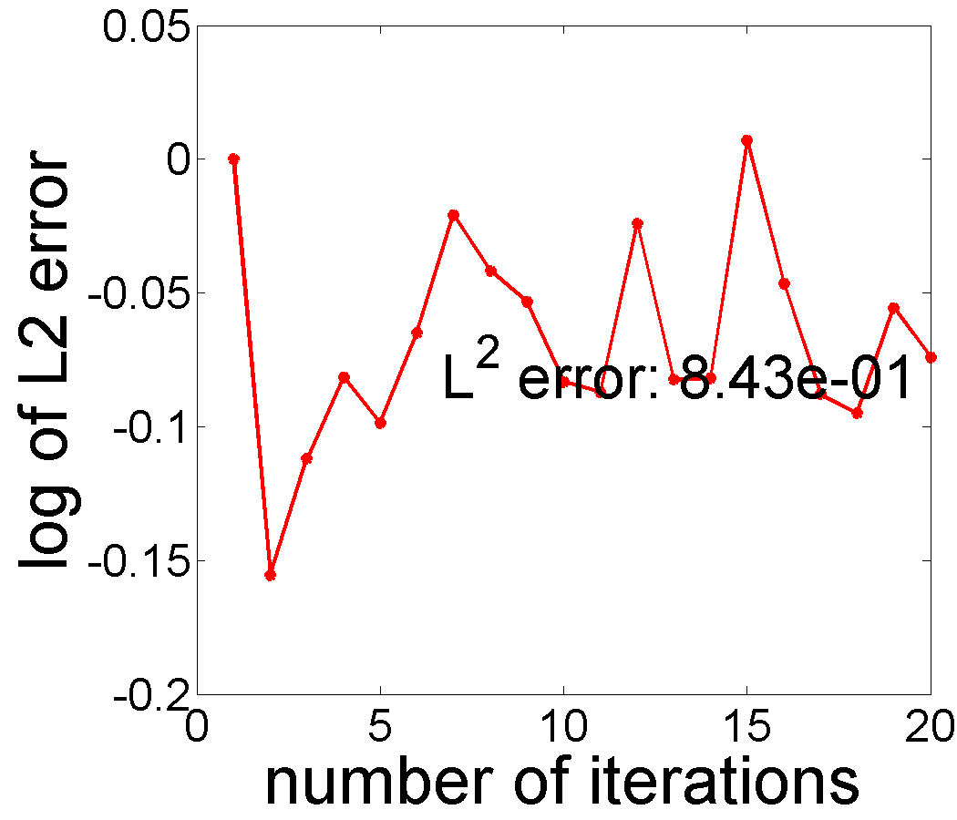 Figure 3
 Figure 4
 Figure 5
 Figure 6
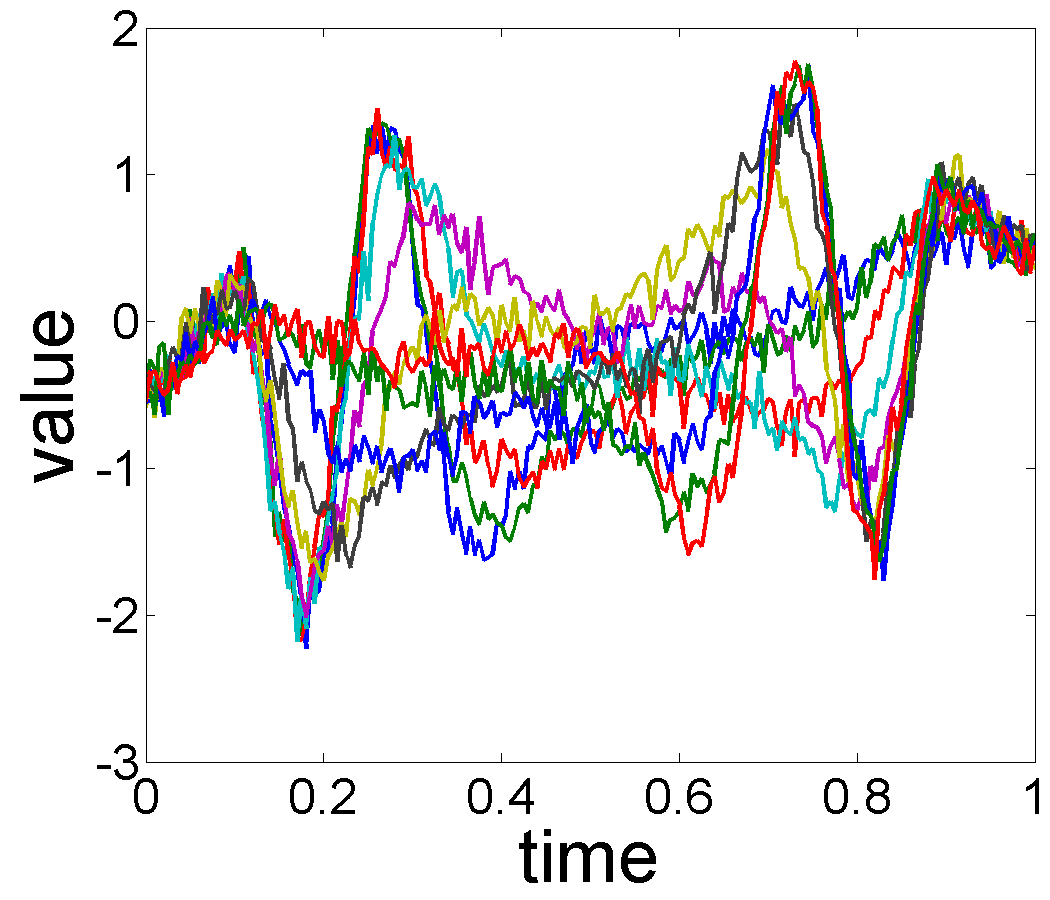 Figure 7
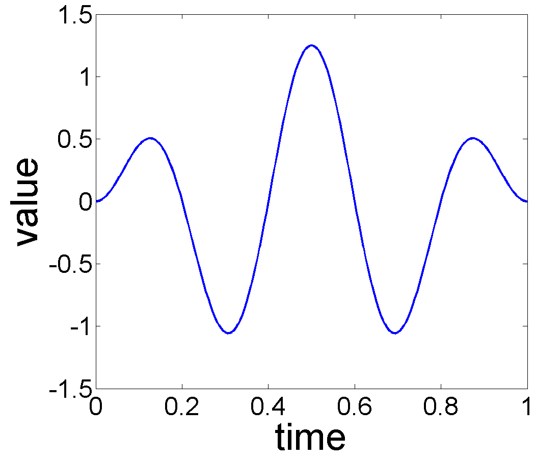 Figure 8
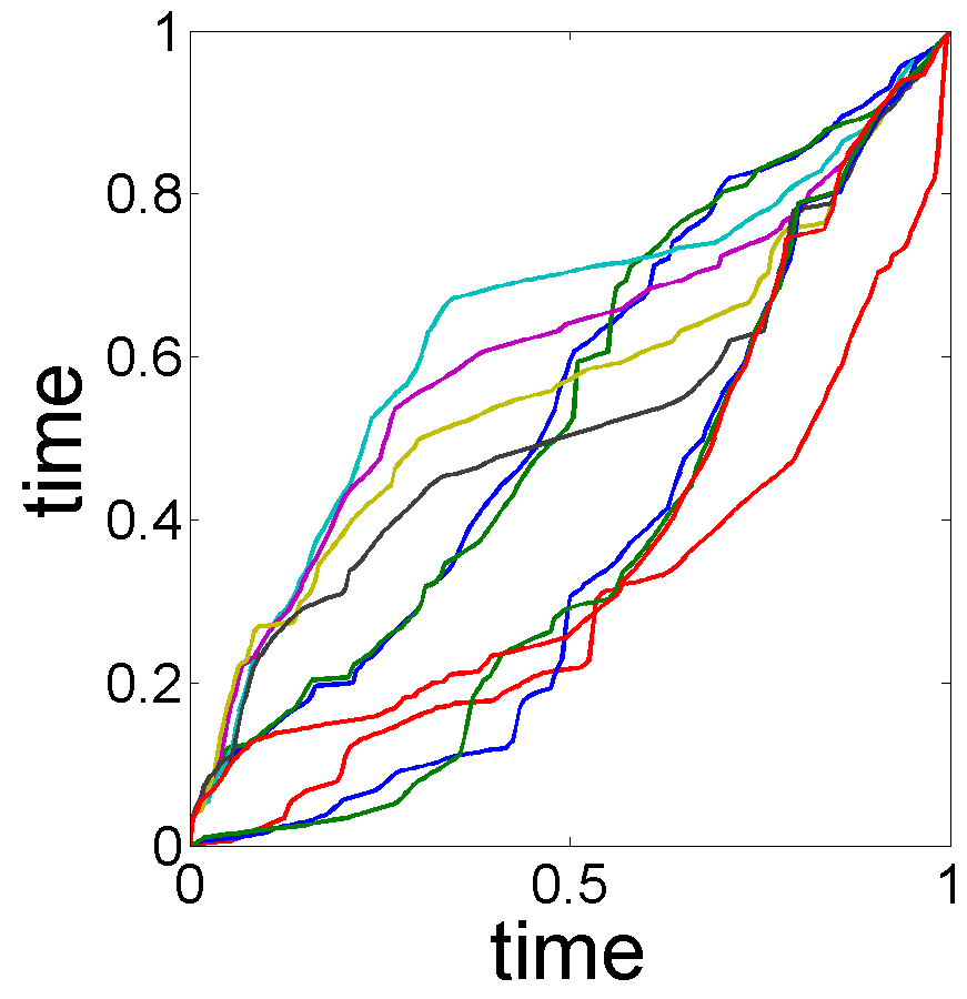 Figure 9
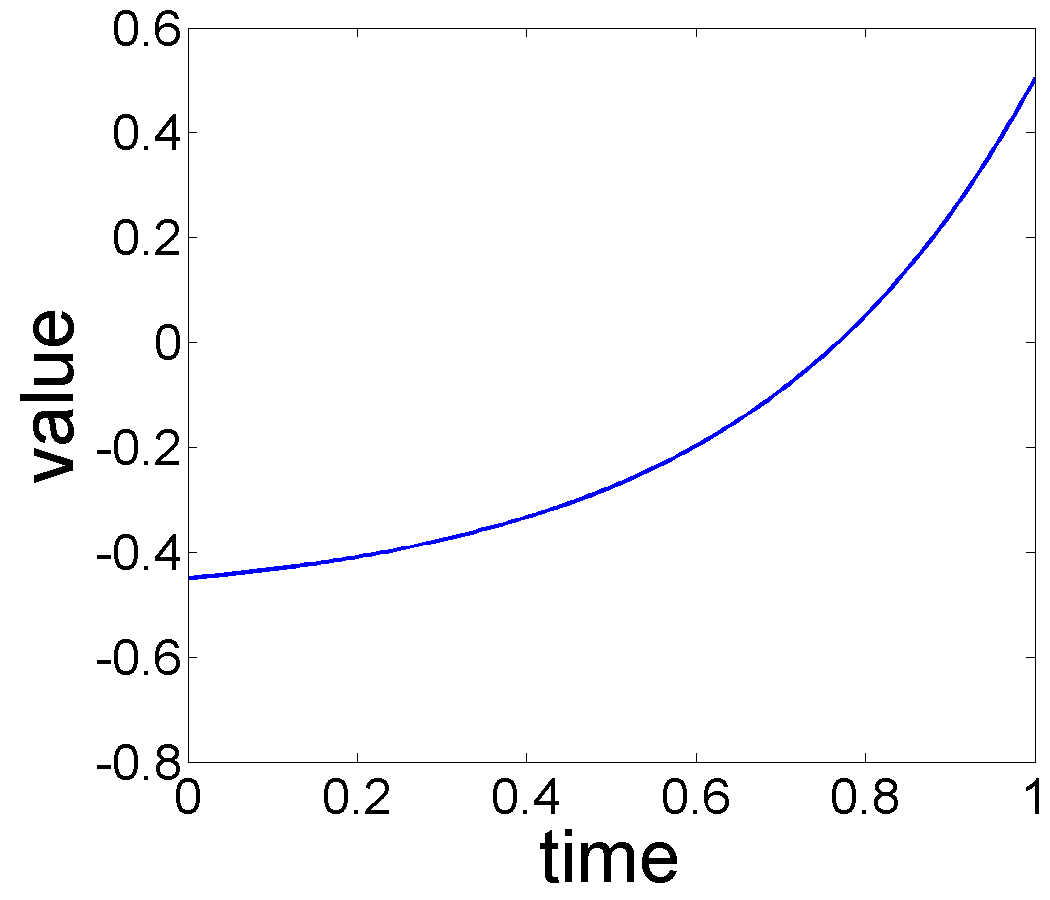 Figure 10
 Figure 11
 Figure 12
 Figure 13
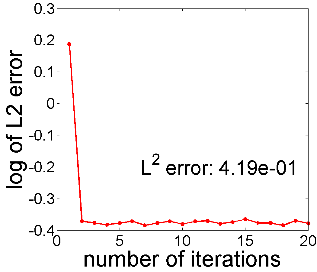 Figure 14
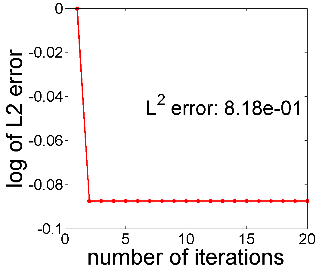 Figure 15
 Figure 16
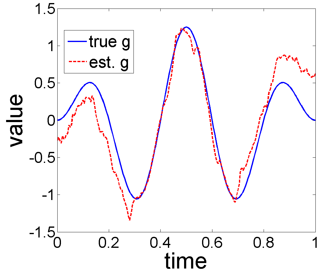 Figure 17
 Figure 18
 Figure 19
 Figure 20
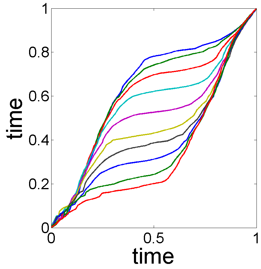 Figure 21
 Figure 22
 Figure 23
 Figure 24
 Figure 25
 Figure 26
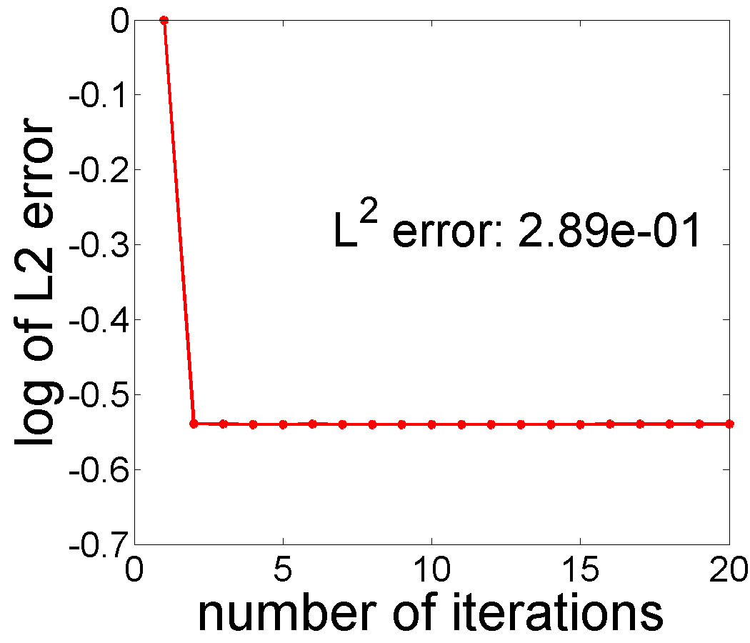 Figure 27
 Figure 28
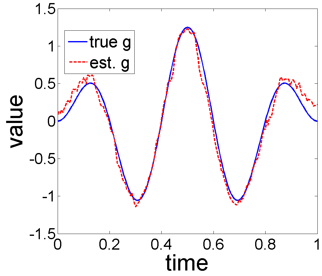 Figure 29
 Figure 30
 Figure 31
 Figure 32
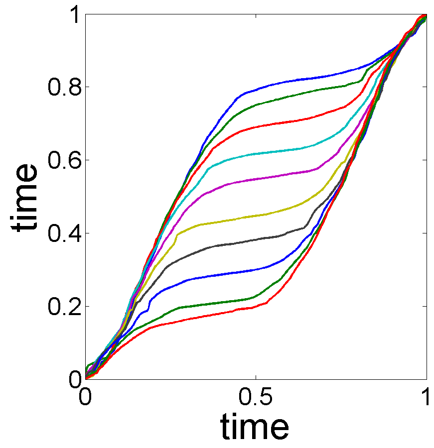 Figure 33
 Figure 34
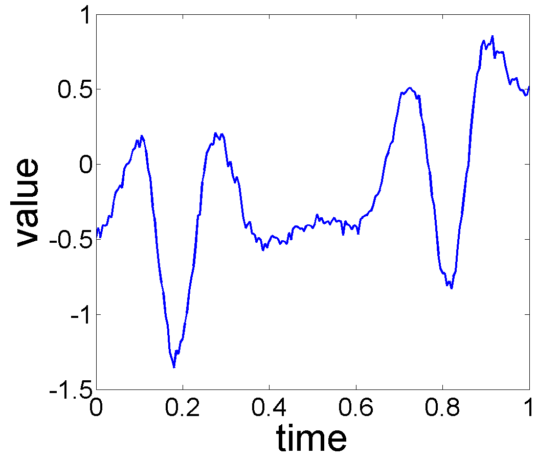 Figure 35
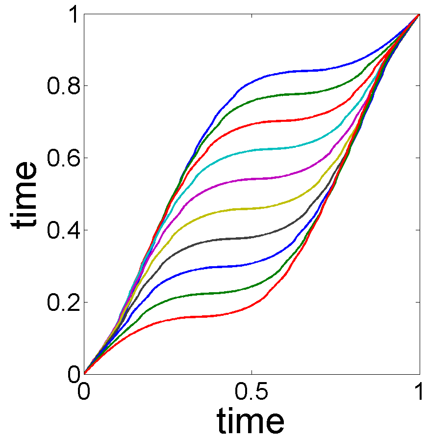 Figure 36
 Figure 37
 Figure 38
 Figure 39
 Figure 40
Peer Reviews
No public reviews on file for this paper yet. If you reviewed it on a platform where reviews are public (OpenReview, ICLR, NeurIPS, ICML), you can paste yours below so the community can read it here.
Videos
No videos yet. Explain this paper in a talk, walkthrough, or lecture? Add one.
Taxonomy
TopicsTime Series Analysis and Forecasting · Statistical and numerical algorithms · Forecasting Techniques and Applications
Trend and Variable-Phase Seasonality Estimation from Functional Data
Liang-Hsuan Tai
Anuj Srivastava
Kyle A. Gallivan
Department of Mathematics, Florida State University, Tallahassee, FL 32306, United States
Department of Statistics, Florida State University, Tallahassee, FL 32306, United States
Abstract
The problem of estimating trend and seasonal variation in time-series data has been studied over several decades, although mostly using single time series. This paper studies the problem of estimating these components from functional data, i.e. multiple time series, in situations where seasonal effects exhibit arbitrary time warpings or phase variability across different observations. Rather than ignoring the phase variability, or using an off-the-shelf alignment method to remove phase, we take a model-based approach and seek MLEs of the trend and the seasonal effects, while performing alignments over the seasonal effects at the same time. The MLEs of trend, seasonality, and phase are computed using a coordinate-descent based optimization method. We use bootstrap replication for computing confidence bands and for testing hypothesis about the estimated components. We also utilize log-likelihood for selecting the trend subspace, and for comparisons with other candidate models. This framework is demonstrated using experiments involving synthetic data and three real data (Berkeley Growth Velocity, U.S. electricity price, and USD exchange fluctuation).
keywords:
Trend and seasonality estimation, Functional Data Analysis , random time warpings , curves registration , alignment
††journal: Computational Statistics and Data Analysis
1 Introduction
We investigate the classical problem of separating trend and seasonal components in a time-series data, but with a few differences. Firstly, we assume the availability of multiple observations, i.e. multiple time series, as opposed to the classical formulation that mostly uses a single time series to perform such estimation. Secondly, we tackle a difficult problem where the seasonal effects exhibit arbitrary time warping, or phase variability (see Marron et al. (2015) for the notion of phase variation), in each observation. This situation arises often in practical situations where the seasonal effect displays cyclostationary behavior, but are seldom aligned perfectly in the observed data.
To make the discussion concrete, let us assume that each individual observation, , is made up of two main components, in addition to the observation noise, according to the superposition model:
[TABLE]
On the right, the different terms are:
- •
Trend, denoted by , captures the long-term evolution of the data. Generally, we are interested in being either a lower order polynomial representing a null, constant, linear, quadratic shapes, or slowly varying sinusoid.
- •
Seasonal effect, denoted by , captures seasonal or period effects in the data, Instead of assuming the seasonal effect to be fixed, or perfectly aligned across observations, we make the model more general by including a temporally-misaligned version of . That is, we utilize the term , instead of , which represents a time warping of by a function , where is a boundary-preserving diffeomorphism. There are several ways to express this warping. The most common form is simply but, as discussed later, there are other possibilities.
- •
Observation noise, denoted by with the assumption that are i. i. d. with for all and .
With this model, the goal is to estimate and using a set of observations . We illustrate this setup pictorially using Fig. 1(a) which shows a set of observed s.
These functions show a periodic behavior, with roughly the same number of peaks and valleys, and a general decreasing trend from left to right. However, the seasonal variations, denoted by high-frequency peaks and valleys, are quite misaligned, implying presence of phase variability in the seasonal components. Traditionally, the seasonal effects are removed by averaging (or smoothing or low-pass filtering) the observed functions across time or observations. A simple cross-sectional average () of the data results in Fig. 1(b). Although this function displays a decreasing trend, it also contains some artifacts that result mainly from the misalignment of seasonal components across individual observations. Therefore, one has to perform an alignment when estimating components in such data. Given the observed functions , a more comprehensive solution is to recover the seasonality , warping functions , and the underlying trend under a statistical model. We will call this problem trend and variable phase seasonality estimation, and a comprehensive solution will isolate the three components, as shown in Fig. 1(c)-(e).
1.1 Past Approaches
Before presenting our model-based solution for trend and seasonality estimation, we summarize the main ideas present in the literature, and point out their limitations and shortcomings. The relevant literature can be divided into the following broad categories, each representing a sub-model of the one presented Eqn. 1.
Estimation from Single Observation: The problem of estimating trend and seasonality from a single time-series originated in Economics (Nerlove (1964) and Godfrey and Karreman (1964)), followed by more formal developments in statistics, see Grether and Nerlove (1970), Cleveland and Tiao (1976), Box et al. (1978), Hillmer and Tiao (1982), Harvey and Todd (1983). Please refer to the review paper by Alexandrov et al. (2012) on this subject, and to U.S. Census Bureau’s website 111http://www.census.gov/srd/www/sapaper/ for a larger list of papers on this topic. Harvey and Todd (1983) formalized the structural time-series model (also termed the classical decomposition model by Brockwell and Davis (2006)) as:
[TABLE]
The goal is to recover the trend and the seasonality , from a single observation . Further special cases of this model result from assuming either or to be zero. Common approaches for estimating trend include parametric least squares (Brockwell and Davis, 2006), moving averages (Brockwell and Davis, 2006), and local linear smoothing (Friedman et al., 2009). On the other hand, the seasonality estimation is often handled by finding cycles (intervals of cyclostationarity) and averaging over those cycles.
For estimating both trend and seasonality, the popular approaches include autoregressive-integrated-moving average (Hillmer and Tiao, 1982, Harvey and Todd, 1983), STL filtering (Cleveland et al., 1990), small trend method (Brockwell and Davis, 2006), moving average estimation (Brockwell and Davis, 2006), and differencing at lag period (Brockwell and Davis, 2006). While these methods are based on the assumption of equally-spaced observations, Eckner (2012) studied the case of unevenly-spaced observations.
Note that none of these models address the issue of temporal misalignment of seasonal effects across cycles. 2. 2.
Trend Estimation Only: In the case where multiple observations are available, one can use techniques from functional data analysis. For instance, one can pose a model of the type:
[TABLE]
Under the zero-mean assumption of , an unconstrained estimator of is the cross-sectional mean, . If is assumed to belong to a certain subspace, say , then there are several techniques available to estimate : B-Splines (Besse et al., 1997), Smoothing Splines (Brumback and Rice, 1998), Basis Functions (Ramsay, 2006), Least Squares (Ramsay, 2006), Roughness Penalty (Ramsay, 2006), and Local Polynomial Kernel (Zhang et al., 2007). This model will perform badly in situations where the data contains some seasonal effects. We mention in passing that although the model used in Ghosh (2001), (), seems different from the one stated above, it is effectively the same given the authors’ assumption that . 3. 3.
Curve Alignment/Seasonal Effect Only: The third related area is registration or alignment of functions. Here, the model does not have a trend component and only considers time warpings of according to:
[TABLE]
Given several observations , the goal here is to remove the effect of and estimate . The simplest case here is pairwise alignment, which was first studied by Sakoe and Chiba (1978) in signal processing. Later on, the problem of aligning multiple functions gained substantial interest in the statistics community with a variety of solutions presented in Kneip and Gasser (1992), Wang and Gasser (1997), Ronn (2001), Liu and Müller (2004), Gervini and Gasser (2004), Ramsay (2006), James (2007), Tang and Muller (2008), Sangalli et al. (2010), Srivastava et al. (2011b); Srivastava and Klassen (2016), Kurtek et al. (2011), Rakêt et al. (2014), and Cheng et al. (2015).
A large majority of these techniques formulate the alignment problem using the standard metric. As pointed out in Marron et al. (2015), this leads to degeneracy in the form of the pinching effect, and also asymmetry in the solution. Srivastava et al. (2011b) (see also Srivastava and Klassen (2016)) presented a natural solution that extends the Fisher-Rao metric to general function spaces and uses a square-root velocity function (SRVF) representation of curves for alignment. This transformation is supported by a fundamental result that the Fisher-Rao Riemannian metric, with its nice invariance properties, transforms to the inner-product under the SRVF transformation. The cross-sectional mean of these aligned SRVFs results in estimation of , see Kurtek et al. (2011) and Cleveland et al. (2016).
In summary, very few of the past papers study the full model given in Eqn. 1 and only estimate some subset of the three components of interest – tread, seasonal effect, and time-warping. The current paper differs from this literature in its consideration of multiple curves, and in estimation of all three components.
1.2 Our Approach
We take a comprehensive approach and explicitly estimate the three components – trend, seasonal effect, and seasonal time warping – using a statistical model. The key idea is to formulate the time-warping of the seasonal component in such a way that the well-known problems of pinching and asymmetry are avoided. This is accomplished by assuming the time warping to be , rather than the traditional , as suggested for SRVFs in Srivastava et al. (2011b) and Srivastava and Klassen (2016). In other words, the model is posed in the SRVF space, rather than the original function space. This warping is norm-preserving, i.e. , with denoting the norm, for any time warping function , and thus has fundamentally better mathematical and computational properties.
Using this warping action, we formulate a statistical model where the observation is a superposition of the trend, the time-warped seasonal effects, and the observation noise. With this model, we formulate a maximum-likelihood estimation problem and solve it using a coordinate-descent algorithm. This requires a critical choice of orthogonal subspaces associated with the trend and (unwarped) seasonal components, and estimating coefficients of these components with respect to the respective bases. Furthermore, we use maximum likelihood to perform model selection in terms of subspace choices, and to compare different candidate models in this problem area. Finally, we use bootstrap to provide confidence bands around estimates of trend and seasonal effects. We illustrate the strength of this framework in formulating hypothesis tests associated with the estimated trends and seasonal effects.
The rest of this paper is organized as follows. In Section 2, we formulate the trend and variable-phase seasonality estimation by a statistical model. Section 3 presents a MLE solution to the model, followed by coordinate-descent optimization and bootstrap analysis. This algorithm requires a pre-determined subspace for the trend and Section 4 develops a rule for selecting this subspace automatically from the data. Section 5 illustrates synthetic and real data examples with a comparison between our MLE algorithm and other models. The paper ends with a conclusion in Section 6.
2 Model-Based Problem Formulation
In order to formulate the problem of trend and seasonality estimation, under time warping of seasonal effects, we particularize Eqn. 1 according to: for ,
[TABLE]
For simplicity, we will assume that is a white Gaussian noise process, with for each independently. (The domain of all functions and is .) The warping functions are assumed to be elements of the set:
[TABLE]
This set has been studied extensively for function and curve representation in shape and functional data analysis (Srivastava et al. (2011a, b); Srivastava and Klassen (2016)). is a group with composition as group operation and the identity element . For each , there exists a unique element such that . We will denote the term by to reduce notation. Note that is the right group action of a group on . We assume that each of the observations and components and are elements of .
Having specified the model, Eqn. 2, we make some assumptions that ensure identifiability of trend and seasonality components.
- •
Consider a simpler case where , for all and the model reduces to . In order to identify and , we require two subspaces , such that , and then we restrict to and . Assuming, as earlier, that , for all and , the estimates of and are given by and , where and are the projections onto and , respectively. This, of course, requires the knowledge of and beforehand.
- •
Now consider the case where s are not identity. In this case, the functions are no longer guaranteed to be in the subspace , i.e. s may have nonzero components in . This underlines the main challenge in the trend and variable-phase seasonality estimation. If had remained orthogonal to , then we could solve the problem using orthogonal projections (or some related smoothing methods). Note that the warping by itself can be handled using the alignment procedures developed in Srivastava et al. (2011b) and Srivastava and Klassen (2016). However, since may not be guaranteed to be orthogonal to , a more sophisticated approach is required to perform the separation.
- •
Another issue here is a lack of identification of , due to its time warping. Since , for any , there is a problem in representing uniquely. This problem can be avoided by assuming an additional constraint on . Srivastava et al. (2011b) suggested forcing the Karcher mean of the inverse warping functions to be the identity, or . (The concept of Karcher mean on is discussed later in Section 3.2.) The similar idea of constraining the mean of warping functions to be was also used in Tang and Muller (2008).
3 Maximum Likelihood Solution
Given observations , and the model stated in Eqn. 1, our goal is to recover the seasonality , warping functions , and the trend , under the assumptions and constraints stated earlier. We will use the maximum-likelihood approach for solving this problem.
3.1 Maximum Likelihood Formulation
To develop a formal estimation setup, start by setting . Let denote a finite partition of representing the observation times. The discrete time samples follow the model . Assuming for each and , the conditional distribution of given is . Since is determined by and , the average log-likelihood of these components, given the observations , is given by:
[TABLE]
Maximizing the above term is the same as minimizing
[TABLE]
In the limit, , the above term becomes
[TABLE]
Thus, finding MLE becomes a problem in constrained functional minimization:
[TABLE]
where is given by .
We reiterate the assumptions that and Karcher Mean are associated with Eqn. 4. Of course, the optimization stated above requires the knowledge of and . We will simplify a little bit by assuming that and, thus, the two choices of and are unified into one. If the subspace is spanned by an orthonormal basis, then the choice of is same as the choice of its basis. Let denote a complete orthonormal basis of . We can choose any subset of and set to be its span. Given , we will assume that for some positive integer . This choice is motivated by the fact that trend is often a slowly varying function over time and first few basis elements should suffice to estimate . Thus, the choice of boils down to the finding an appropriate .
3.2 Optimization Using Coordinate-Descent
We will use a coordinate-descent method for solving Eqn. 4. This optimizes along one direction/variable at a time, and iterates until we reach a stationary point. To apply the coordinate-descent method to our problem, we need to derive each of the following items:
Update trend : Given the current estimates and , the estimate for is as follows:
[TABLE]
where is an orthogonal basis of and denotes the standard inner product. We consider the following bases in this paper: Fourier basis , sine basis , cosine basis , and shifted Legendre basis (see Kreyszig (1989))
[TABLE] 2. 2.
Update seasonality : Given and , the update for is defined as follows:
[TABLE]
The last equality uses the fact that , see Srivastava et al. (2011b). Hence, the optimization problem is simplified into a vector space optimization under subspace and the minimizer for is
[TABLE] 3. 3.
Update warping functions : Given the estimates of and , this problem can be rephrased as:
[TABLE]
with Karcher mean constraint Notice that are independent of each other in their contributions to the cost function in Eqn. 7. Therefore, we solve the optimization problem as an unconstrained one and then impose the Karcher mean constraint. For each , we solve for:
[TABLE]
This can be solved using Dynamic Programming technique (Bellman, 1954). The computation of the Karcher mean of warping functions , under the Fisher-Rao metric, has been provided in Algorithm 1 of the paper Srivastava et al. (2011b) and Section 7.5 of the textbook Srivastava and Klassen (2016). By using Lemma 4 in Srivastava et al. (2011b), the mean constraint is imposed by setting The procedure for solving the constrained functional optimization (Eqn. 7) with the condition is summarized in Algorithm 1.
Given updates for variables , , and in Eqn. 5, Eqn. 6, and Algorithm 1, the coordinate-descent method yields Algorithm 2.
Fig. 2 shows two examples of using Algorithm 2 on simulated data. In the top case the estimated trend is monotonic increasing while in the bottom case it first decreases and then increases.
3.3 Bootstrap Analysis: Confidence Regions and Testing
Given the complexity of the data model, and the subsequent estimators, it is difficult to derive analytical expressions for asymptotic distributions of the estimated quantities. Therefore, we take a bootstrap approach and compute estimator statistics using random replication, and use these statistics for testing hypotheses about trend and seasonality. In the following, we present details for computing bootstrap estimates of standard deviations of certain test statistics. These statistics, in turn, can be used to test important hypotheses, such as the presence or absence of a trend or a seasonality component in the observed data.
Hypothesis Testing for Trend and Seasonality: An important and challenging problem in functional data analysis is to test the presence of a trend in the given data. That is, given a set of functions , we can pose the question: Is , or not? This leads to a formal binary hypothesis test, with null hypothesis : and the alternative hypothesis : . In view of the implicit assumptions about continuity of (due to the condition that , a subspace of smooth functions), we have that is equivalent to . Therefore, we define a test statistic and rewrite the hypothesis test as: null hypothesis : and the alternative hypothesis : . Let denote the bootstrap replicate of the estimator , and let denote its norm. Furthermore, let be the standard error of using replicates. Then, we can compute the value of the test statistic assuming a normal distribution under the null hypothesis.
In fact, one can use the bootstrap procedure to test any specific shape pattern of the trend and seasonality function. For instance, one can test the trend function for being constant, linear, or monomial of certain order. As an example, we can test if the trend is a constant function by modifying the test statistic to be . Note that there are other choices possible for the test statistic in this case (for example ) but we have chosen one arbitrarily here. A test statistic for testing the linearity of the trend is .
Bootstrap Cross-Sectional Confidence Band: In addition to providing point estimates of and in their respective subspaces, one can use bootstrap to provide a confidence region associated with these estimates. The basic idea is to take bootstrap replicates of the estimator and use the norm to build confidence regions around the estimate, for either and . Since under the metric, the mean of functions corresponds to a cross-sectional mean, this task simplifies to building a confidence interval at each time . We use the bootstrap replicates to arrive at these confidence intervals. Let and be the bootstrap averages, and and be the bootstrap estimates of the standard errors, as functions of , of and , respectively. For a significance level , the confidence interval for is simply , where is the th percentile point of a standard normal distribution. Similarly, the confidence interval for the estimated seasonal effect is simply . Examples of bootstrap-based analysis are shown later in this paper.
4 Trend Subspace Selection
So far in this framework we have assumed that , the subspace of associated with the trend, is known. Since need not choose separately, we only need to choose . The next question is: How to infer the subspace automatically from the data? It turns out that the current framework also provides a criterion for choosing between potential candidates, by simply maximizing the likelihood under each candidate subspace and selecting the one that results in the highest maximized-likelihood. Earlier we assumed that for some positive integer . Thus, the choice of boils down to the finding an appropriate . With this setting, we can try each potential value of , up to a certain large value, maximize the likelihood under each choice of , and selecting the one with the highest value of the likelihood (or, correspondingly the smallest value of negative log-likelihood in Eqn. 4).
Remark 1**.**
We point out that this approach of selecting will not work if we ignore the phase variability in the seasonal component, or set for all . For instance, we assume the model , and use the natural estimators and for and , respectively, then the negative log-likelihood will remain unchanged with the changes in . Subspace selection using log-likelihood will work only when we have non-trivial warpings.
We demonstrate this idea using a simulated example. In this experiment, we generate data using
, , and where for , with the additional constraint that . We add noise according to , in this experiment. The resulting data are shown in Fig. 3(d).
We apply Algorithm 2 to this data for , and , and the results are presented in the Fig. 4. The s used in this experiment come from the shifted Legendre polynomial basis and the trend is thus a polynomial of degree . From a visual perspective, setting yields the best estimates of and . Fig. 5 displays the minimized negative log-likelihood for to and the optimal is obtained when , supporting our approach for selecting . This selection rule can be generalized to the situations when several potential basis types (polynomial, sine, cosine, Fourier) are given.
5 Experimental Results
In this section we present some results for estimating the trend and seasonal components using the MLE algorithm specified earlier. We will use both the synthetic and real datasets to illustrate the ideas.
5.1 Synthetic Data
Performance Under Different Noise Levels: In this experiment, we select a specific form of the trend and seasonal components, and increase the variance, , of the additive noise to study the effect of noise on estimation performance. In this experiment we used , , and warping functions , where . For each , we consider Gaussian noise where is and for the noise level experiments. Each observation is generated from Eqn. 2 and the number of time samples is taken to be . Fig. 6 shows the true trend and the seasonal components, when no noise is added. Fig. 7 displays estimation results for the additive noise levels.
As shown in Fig. 7, the estimation results are very good when the noise level is relatively low (), with the relative error , and for , , and respectively. When the noise increases to and , the reconstructed trends still have the desired pattern over but the recovered seasonality results are not good as noise level . With large noise, , all the estimated results are far from their truth values. These experiments provide evidence that the MLE algorithm can recover good estimates of the trend, seasonality and warping functions in the presence of some levels of noise. 2. 2.
Illustration of Testing Using Bootstrap: In this experiment, we illustrate the use of a bootstrap technique for testing different hypotheses associated with the shapes of estimated trend and seasonal effect. The general idea was described in Section 3.3 and it is applied here to the data shown in Fig. 1. In this data, we have used , , and for . Additionally, we set . The estimated trend and seasonality components are in Fig. 1. Fig. 8, (a) and (b), shows the bootstrap replicates and of the trend and seasonality estimates for . As these replicates indicate, there is a significant phase variation in the replicates and relatively small variability in the replicates . The bootstrap technique yields the following results:
- •
Testing presence of a trend: For testing , the test statistic using bootstrap is with and a value of 0. The null hypothesis is therefore rejected.
- •
Testing constant shape for a trend: For testing , the test statistic using bootstrap is with and a value of 0. Therefore, we reject the null hypothesis: .
- •
Testing linear shape for a trend: For the linearity of a trend, we obtain , , and a value of 0. Thus, we reject the null hypothesis: is a linear function.
The cross-sectional confidence bands with confidence level in Fig. 8, (c) and (d), indicate that the estimator is much better than the .
5.2 Real Data
5.2.1 Berkeley Male Growth Velocity
The Berkeley Growth Study of 54 females and 39 males was performed by Tuddenham and Snyder (1954) and further discussed by Ramsay (2006). As an example, 10 out of 39 male growth curves are shown in Fig. 9(a). Due to the monotonic nature of the curve, researchers often analyze the time derivative, termed the growth velocity, shown in Fig. 9(b). Looking at these growth curves, one can discern some patterns of high growth, termed growth spurts, for all subjects. However, naturally these spurts are not synchronized across subjects, i.e. they occur at different times for different subjects. Additionally, there is a downward trend in the growth velocities across all subjects. Our goal is to estimate the overall trend and the seasonal effect in this velocity data, and to test their significance.
For this data, our subspace selection finds the optimal trend subspace to be . The estimated trend and seasonal components for this are shown in Fig. 10. As we can see, our algorithm detects a near-linear decay in growth velocity with age and a growth spurt around age 13.
For comparison purposes, the trend estimation results of applying the separation model are shown in Fig. 11. This method requires a specification of , and the results are sensitive to this choice. Recall from Remark 1, this approach cannot select , as is done in our MLE algorithm. Clearly the results do not capture the expected properties of the trend. Due to the lack of phase variability in the separation model, the estimates of do not capture the desired growth spurt and not presented in the paper.
The bootstrap technique yields the following results:
- •
Testing presence of a trend: When testing for the null hypothesis using the bootstrap technique, we get , , and a value of . As a result, we reject the null hypothesis.
- •
Testing constant shape for a trend: When testing for null hypothesis , the test statistic is with . Since the corresponding value is , we reject the null hypothesis: .
- •
Testing linear shape for a trend: When testing the linearity of a trend, we obtain test statistic with , and a value of 0.37. We fail to reject that the null hypothesis: the trend is a linear. This conclusion is consistent with Fig. 10(a).
Finally, Fig. 12, (a) and (b), shows cross-sectional confidence bands for and at confidence level.
5.2.2 U.S. Electricity Price
This example studies the monthly U.S. electricity prices for years 2005 to 2010, with data as shown in the left panel of Fig. 13. The -axis represents time on a monthly scale from 2005.1 to 2010.12. The -axis is unit price of electricity in cents per kilowatt-hour. According to the data source, the U.S. Energy Information Administration 222http://www.eia.gov/electricity/data.cfm, divides U.S. into several regions: Alaska, Hawaii, New England, Middle Atlantic, East North Central, West North Central, South Atlantic, East South Central, West South Central, Mountain, Pacific Contiguous and Pacific Non-contiguous. We restrict to six regions in this analysis since these regions use the same electricity generation method. The raw data is shown in the left panel of Fig. 13. In this data, we clearly see a seasonal effect on a yearly basis – electricity prices increase during the summer and fall back during the winter. Since there are six annual cycles in the data, we expect six peaks in the estimated seasonality . Also, as the cycles are not quite synchronized, there is a potential for phase variability in the seasonal effect. Notice that there is a slowly increasing pattern from 2005 to 2010, pointing to the presence of a trend in the data.
We applied our subspace selection approach to this data, and found the optimal choice of trend subspace is . With this choice of , the MLE of the trend and seasonal effects are shown in Fig. 13, (a) and (b). The trend estimation results of the separation model with different choices of are shown in Fig. 14. While some results (Fig. 14(c) and Fig. 14(e)) seem decent, we do not have a way of selecting one over the other. Moreover, since the lack of phase variability in the separation model, the estimates of do not process the desired seasonal oscillation.
We now turn to bootstrap hypothesis testing of the results to the MLE algorithm.
- •
Testing presence of a trend: For testing if the trend is null, we obtain test statistic with . The associated value is 0 and this trend is not null.
- •
Testing constant shape for a trend: For testing null hypothesis , we obtain test statistic and its bootstrap standard error . The value is so we fail to reject that the null hypothesis: trend is a constant.
- •
Testing linear shape for a trend: For testing the linearity of a trend , we have and . We fail to reject the null hypothesis, is linear, since a large value 0.47.
The cross-sectional confidence bands with 95% confidence level for and , are shown in Fig. 15 for the electricity price data.
5.2.3 U.S. Currency Exchange Fluctuation
In this experiment, we consider an application of financial data. The US dollar foreign exchange rates from October 2015 to December 2015 are shown in Figure 16(a). In finance, exchange fluctuation is studied rather than using exchange rates. The exchange fluctuation is defined as where is the current exchange rate and is the previous exchange rate. If the number is positive, the US dollar is undergoing revaluation and a negative value means devaluation. Figure 16(b) displays the USD exchange fluctuation. The analysis of exchange fluctuation is harder than Growth Velocity data and electricity price data since there is no physical interpretation. Moreover, the observed currency behavior may be related to less quantifiable considerations such as economic policies and governments.
Our MLE algorithm selects the trend space and produces the estimated trend and seasonal effects given in Fig. 17. The estimated trend has a slow oscillation, while the estimated seasonal effect oscillates with a significantly higher frequency. Applying the separation model to the data yields the estimated trends shown in Fig. 18. While the trends in Fig. 18, (c)-(e), seems reasonable, the lack of physical interpretation of the data and the inability to select the subspace due to the invariance of the negative log-likelihood function, it is not possible to quantify the selection of these trends.
Bootstrapping hypothesis testing for the currency fluctuation yields the following:
- •
Testing presence of a trend: For testing the null hypothesis , we have , , and a value of . Therefore we reject the null hypothesis.
- •
Testing constant shape for a trend: For testing the null hypothesis, , the test statistic using bootstrap is with . The corresponding value is and therefore, the null hypothesis is rejected.
- •
Testing linear shape for a trend: For testing the linearity of a trend, the test statistic using bootstrap is with . Since the value is , we fail to reject the null hypothesis.
Finally, Fig. 19 shows cross-sectional confidence bands for the trend and the seasonality at the 95 confidence level.
6 Conclusion
We have developed a novel, model-based framework to solve the trend and variable phase seasonality estimation problem by estimating the trend and seasonality components from time series data, in situations where the seasonal component exhibits random time warpings. The model subsumes those used by related approaches in the literature. We assume that the subspaces associated with these two components – trend and seasonality – are orthogonal, and the Karcher mean of warping functions is identity, to ensure that the components are identifiable. Under these conditions we seek MLE of and , using a coordinate-descent algorithm that iteratively updates one component at a time, while fixing the others. We also use maximized likelihood to select an appropriate subspace for the trend component using a increasing sequence of nested subspaces. The estimated quantities – trend and seasonality – are tested, using bootstrap replication, for being null or having a specific simple shape, such as constant and linear.
Both synthetic data and real data have been used to demonstrate the effectiveness of this method. Using synthetic data, where the ground truth is known, we have demonstrated the robustness of our method in the presence of noise. We demonstrate this framework’s ability to extract trend and seasonality using three real application datasets: the Berkeley Growth data, U.S. electricity price data, and USD exchange fluctuation. Bootstrap hypothesis testing supported the presence of a trend in all of the datasets. For the USD exchange fluctuation data, a low frequency oscillation between revaluation and devaluation was extracted, along with a higher frequency seasonal oscillation. For the Berkeley Growth data and electricity price data, we obtain estimates of the trends and seasonal effects that are expected from the nature of the applications.
References
- Alexandrov et al. (2012)
Alexandrov T, Bianconcini S, Dagum EB, Maass P, McElroy TS.
A review of some modern approaches to the problem of trend extraction.
Econometric Reviews 2012;31(6):593–624.
- Bellman (1954)
Bellman R.
The theory of dynamic programming.
Technical Report; DTIC Document; 1954.
- Besse et al. (1997)
Besse PC, Cardot H, Ferraty F.
Simultaneous non-parametric regressions of unbalanced longitudinal data.
Computational Statistics & Data Analysis 1997;24(3):255–70.
- Box et al. (1978)
Box GE, Hilimer S, Tiao GC.
Analysis and modeling of seasonal time series.
In: Seasonal analysis of economic time series. NBER; 1978. p. 309–44.
- Brockwell and Davis (2006)
Brockwell PJ, Davis RA.
Introduction to time series and forecasting.
Springer Science & Business Media, 2006.
- Brumback and Rice (1998)
Brumback BA, Rice JA.
Smoothing spline models for the analysis of nested and crossed samples of curves.
Journal of the American Statistical Association 1998;93(443):961–76.
- Cheng et al. (2015)
Cheng W, Dryden IL, Huang X, et al.
Bayesian registration of functions and curves.
Bayesian Analysis 2015;.
- Cleveland et al. (2016)
Cleveland J, Wu W, Srivastava A.
Norm-preserving constraint in the Fisher–Rao registration and its application in signal estimation.
Journal of Nonparametric Statistics 2016;28(2):338–59.
- Cleveland et al. (1990)
Cleveland RB, Cleveland WS, McRae JE, Terpenning I.
Stl: A seasonal-trend decomposition procedure based on loess.
Journal of Official Statistics 1990;6(1):3–73.
- Cleveland and Tiao (1976)
Cleveland WP, Tiao GC.
Decomposition of seasonal time series: A model for the census x-11 program.
Journal of the American statistical Association 1976;71(355):581–7.
- Eckner (2012)
Eckner A.
A note on trend and seasonality estimation for unevenly-spaced time series.
- Friedman et al. (2001)
Friedman J, Hastie T, Tibshirani R.
The elements of statistical learning.
volume 1.
Springer series in statistics Springer, Berlin, 2001.
- Gervini and Gasser (2004)
Gervini D, Gasser T.
Self-modelling warping functions.
Journal of Royal Statistics Society 2004;66 part 4:959–71.
- Ghosh (2001)
Ghosh S.
Nonparametric trend estimation in replicated time series.
Journal of statistical planning and inference 2001;97(2):263–74.
- Godfrey and Karreman (1964)
Godfrey MD, Karreman HF.
A spectrum analysis of seasonal adjustment.
Citeseer, 1964.
- Grether and Nerlove (1970)
Grether DM, Nerlove M.
Some properties of optimal seasonal adjustment.
Econometrica: Journal of the Econometric Society 1970;:682–703.
- Harvey and Todd (1983)
Harvey AC, Todd P.
Forecasting economic time series with structural and Box-Jenkins models: A case study.
Journal of Business & Economic Statistics 1983;1(4):299–307.
- Hillmer and Tiao (1982)
Hillmer SC, Tiao GC.
An ARIMA-model-based approach to seasonal adjustment.
Journal of the American Statistical Association 1982;77(377):63–70.
- James (2007)
James GM.
Curve alignment by moments.
The Annals of Applied Statistics 2007;1 No.2:480–501.
- Kneip and Gasser (1992)
Kneip A, Gasser T.
Statistical tools to analyze data representing a sample of curves.
The Annals of Statistics 1992;20 No. 3:1266–305.
- Kreyszig (1989)
Kreyszig E.
Introductory functional analysis with applications.
volume 1.
wiley New York, 1989.
- Kurtek et al. (2011)
Kurtek SA, Srivastava A, Wu W.
Signal estimation under random time-warpings and nonlinear signal alignment.
In: Advances in Neural Information Processing Systems. 2011. p. 675–83.
- Liu and Müller (2004)
Liu X, Müller HG.
Functional convex averaging and synchronization for time-warped random curves.
Journal of the American Statistical Association 2004;99(467):687–99.
- Marron et al. (2015)
Marron JS, Ramsay JO, Sangalli LM, Srivastava A, et al.
Functional data analysis of amplitude and phase variation.
Statistical Science 2015;30(4):468–84.
- Nerlove (1964)
Nerlove M.
Spectral analysis of seasonal adjustment procedures.
Econometrica: Journal of the Econometric Society 1964;:241–86.
- Rakêt et al. (2014)
Rakêt LL, Sommer S, Markussen B.
A nonlinear mixed-effects model for simultaneous smoothing and registration of functional data.
Pattern Recognition Letters 2014;38:1–7.
- Ramsay (2006)
Ramsay JO.
Functional data analysis.
Wiley Online Library, 2006.
- Ronn (2001)
Ronn B.
Nonparametric maximum likelihood estimation for shifted curves.
Journal of Royal Statistics Society 2001;63, Part 2:241–59.
- Sakoe and Chiba (1978)
Sakoe H, Chiba S.
Dynamic programming algorithm optimization for spoken word recognition.
IEEE Transactions on Acoustics, Speech, and Signal Processing 1978;ASSP-26(1):43–9.
- Sangalli et al. (2010)
Sangalli LM, Secchi P, Vantini S, Vitelli V.
K-mean alignment for curve clustering.
Computational Statistics and Data Analysis 2010;54:1219–33.
- Srivastava and Klassen (2016)
Srivastava A, Klassen E.
Functional and shape data analysis.
Springer Series in Statistics, 2016.
- Srivastava et al. (2011a)
Srivastava A, Klassen E, Joshi S, Jermyn I.
Shape analysis of elastic curves in Euclidean space.
IEEE Transactions on Pattern Analysis and Machine Intelligence 2011a;33:1415–28.
- Srivastava et al. (2011b)
Srivastava A, Wu W, Kurtek S, Klassen E, Marron J.
Registration of functional data using Fisher-Rao metric.
arXiv:11033817 2011b;.
- Tang and Muller (2008)
Tang R, Muller HG.
Pairwise curve synchronization for functional data.
Biometrika 2008;95:4:875–89.
- Tuddenham and Snyder (1954)
Tuddenham RD, Snyder MM.
Physical growth of california boys and girls from birth to eighteen years.
Publications in child development University of California, Berkeley 1954;1(2):183.
- Wang and Gasser (1997)
Wang K, Gasser T.
Alignment of curves by dynamic time wapring.
The Annals of Statistics 1997;25 No.3:1251–76.
- Zhang et al. (2007)
Zhang JT, Chen J, et al.
Statistical inferences for functional data.
The Annals of Statistics 2007;35(3):1052–79.
The reference list from the paper itself. Each links out to its DOI / PubMed record.
- 1Alexandrov et al. (2012) Alexandrov T, Bianconcini S, Dagum EB, Maass P, Mc Elroy TS. A review of some modern approaches to the problem of trend extraction. Econometric Reviews 2012;31(6):593–624.
- 2Bellman (1954) Bellman R. The theory of dynamic programming. Technical Report; DTIC Document; 1954.
- 3Besse et al. (1997) Besse PC, Cardot H, Ferraty F. Simultaneous non-parametric regressions of unbalanced longitudinal data. Computational Statistics & Data Analysis 1997;24(3):255–70.
- 4Box et al. (1978) Box GE, Hilimer S, Tiao GC. Analysis and modeling of seasonal time series. In: Seasonal analysis of economic time series. NBER; 1978. p. 309–44.
- 5Brockwell and Davis (2006) Brockwell PJ, Davis RA. Introduction to time series and forecasting. Springer Science & Business Media, 2006.
- 6Brumback and Rice (1998) Brumback BA, Rice JA. Smoothing spline models for the analysis of nested and crossed samples of curves. Journal of the American Statistical Association 1998;93(443):961–76.
- 7Cheng et al. (2015) Cheng W, Dryden IL, Huang X, et al. Bayesian registration of functions and curves. Bayesian Analysis 2015;.
- 8Cleveland et al. (2016) Cleveland J, Wu W, Srivastava A. Norm-preserving constraint in the Fisher–Rao registration and its application in signal estimation. Journal of Nonparametric Statistics 2016;28(2):338–59.