Representative galaxy age-metallicity relationships
Andr\'es E. Piatti, Antonio Aparicio, Sebasti\'an L. Hidalgo

TL;DR
This paper introduces a fast method for deriving approximate galaxy age-metallicity relationships from color-magnitude diagrams, enabling efficient analysis of large galaxy surveys.
Contribution
The paper presents a quick-look approach to determine galaxy AMRs using representative ages and metallicities, reducing computational demands compared to traditional methods.
Findings
Reliable down to >85% photometric completeness
Accurately traces chemical evolution for stellar populations within 40% mass of the main population
Effective across a wide range of galaxy star formation histories
Abstract
The ongoing surveys of galaxies and those for the next generation of telescopes will demand the execution of high-CPU consuming machine codes for recovering detailed star formation histories (SFHs) and hence age-metallicity relationships (AMRs). We present here an expeditive method which provides quick-look AMRs on the basis of representative ages and metallicities obtained from colour-magnitude diagram (CMD) analyses. We have tested its perfomance by generating synthetic CMDs for a wide variety of galaxy SFHs. The representative AMRs turn out to be reliable down to a magnitude limit with a photometric completeness factor higher than 85 per cent, and trace the chemical evolution history for any stellar population (represented by a mean age and an intrinsic age spread) with a total mass within ~ 40 per cent of the more massive stellar population in the galaxy.
Click any figure to enlarge with its caption.
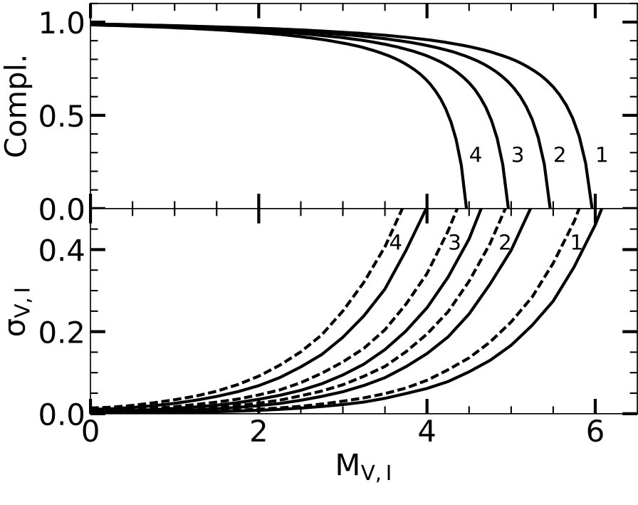 Figure 1
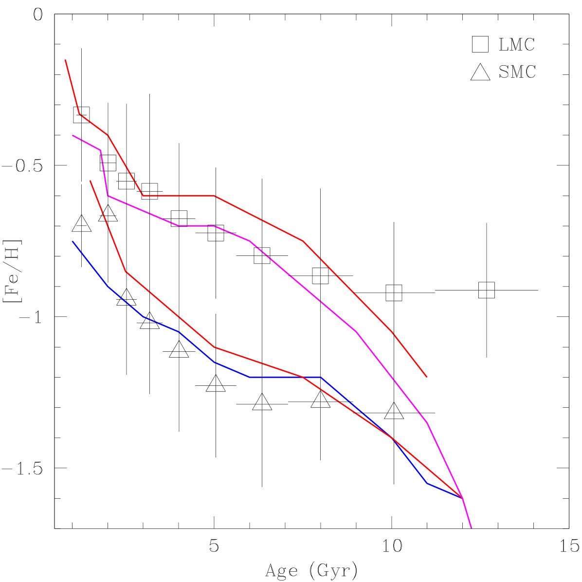 Figure 1
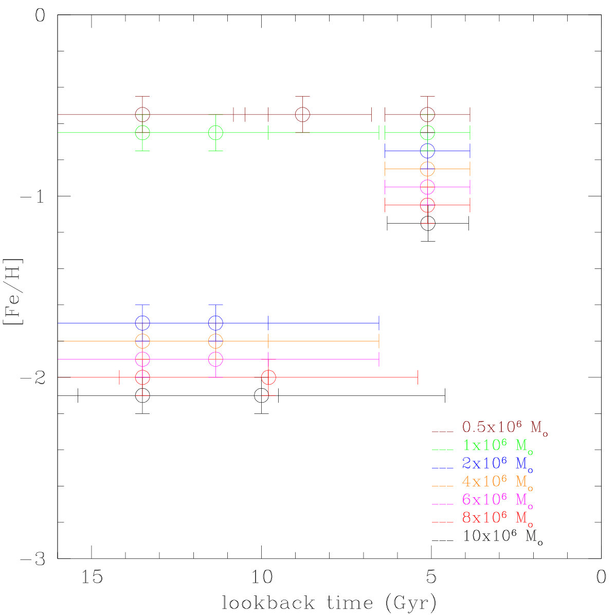 Figure 10
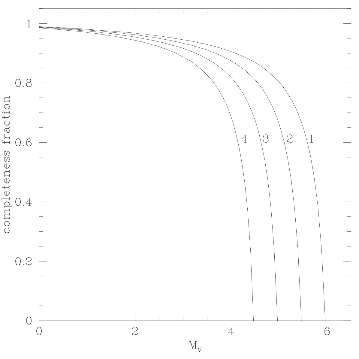 Figure 2
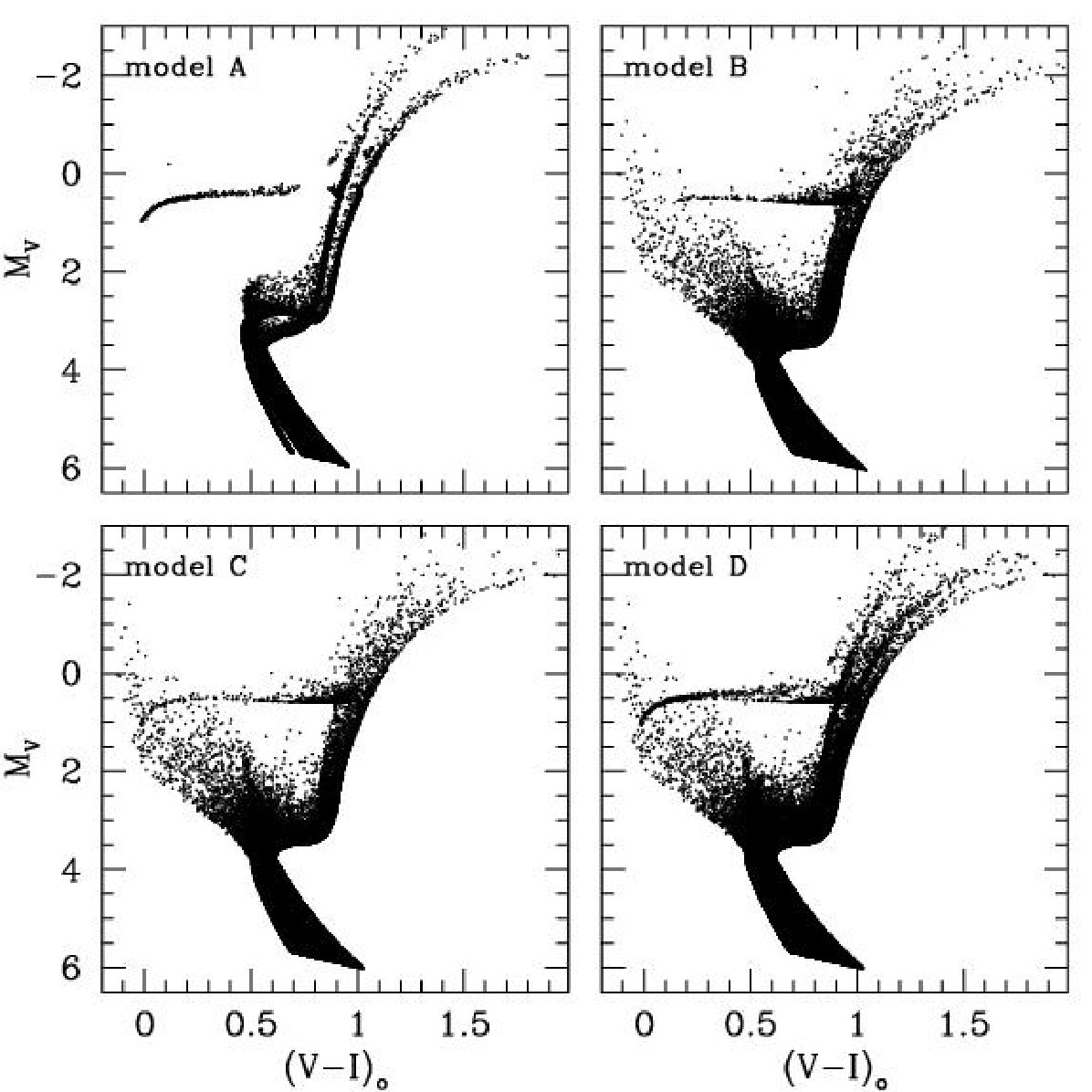 Figure 3
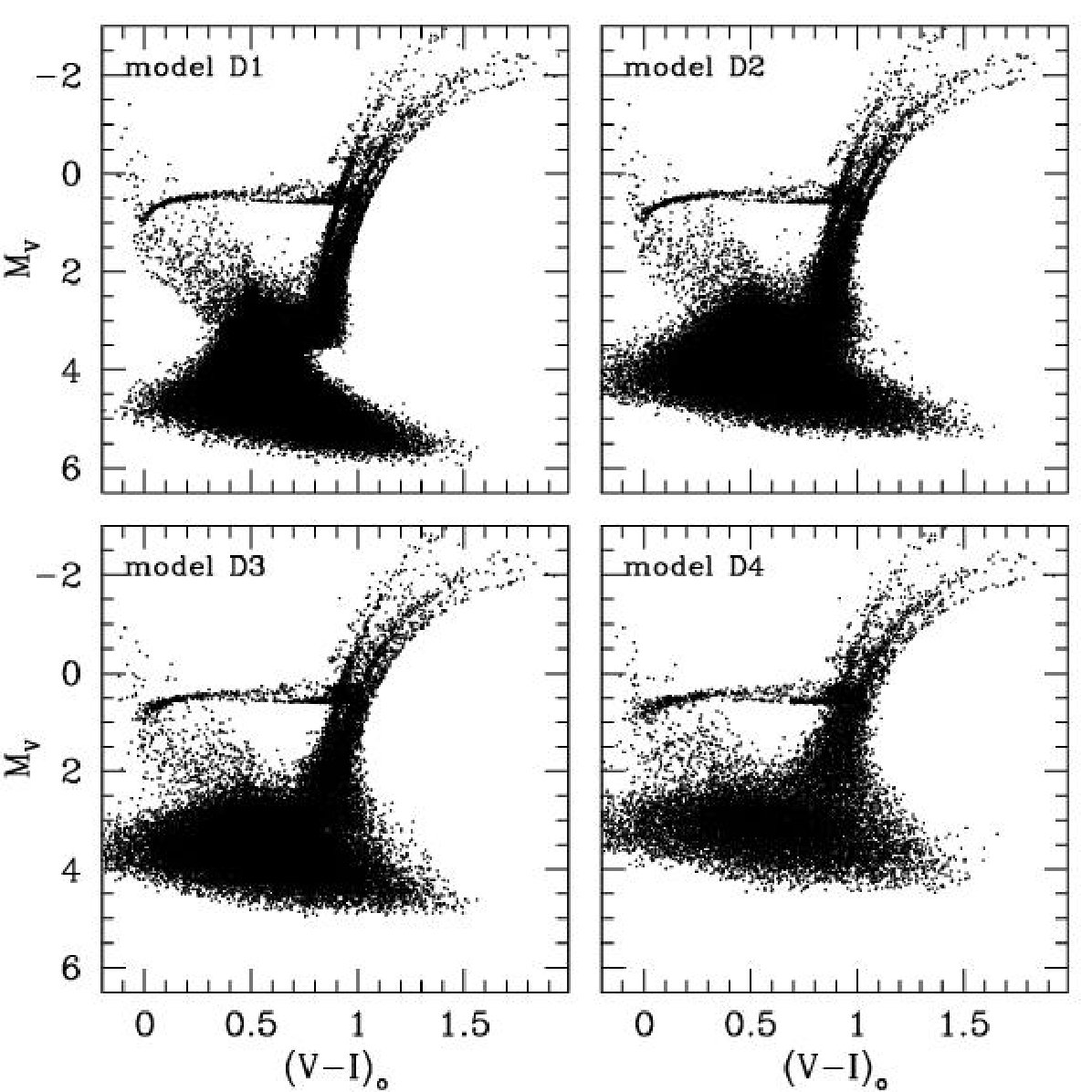 Figure 4
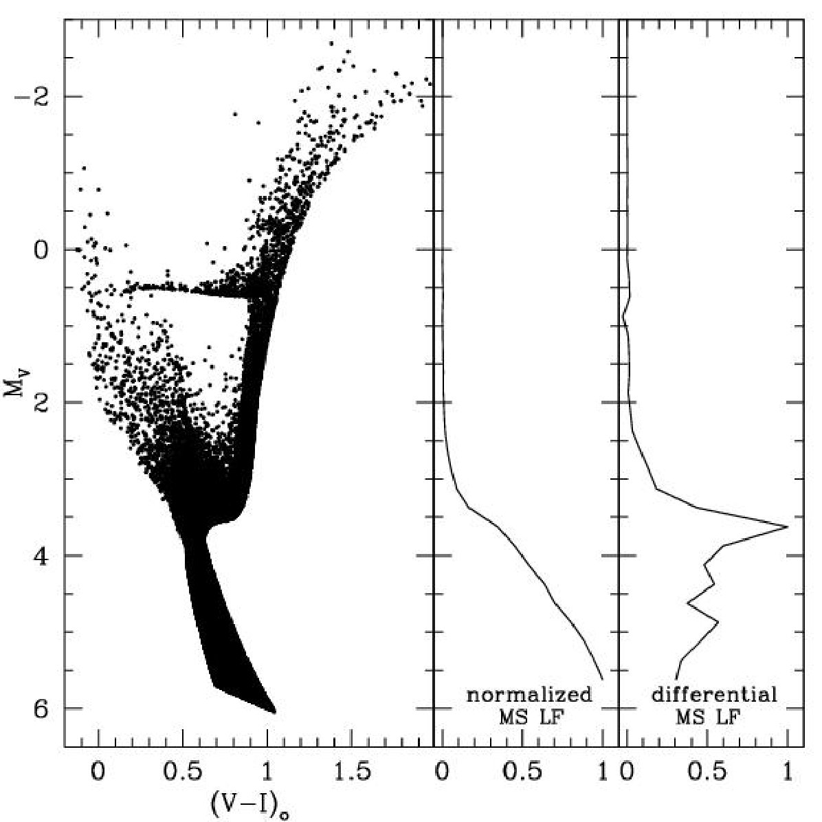 Figure 5
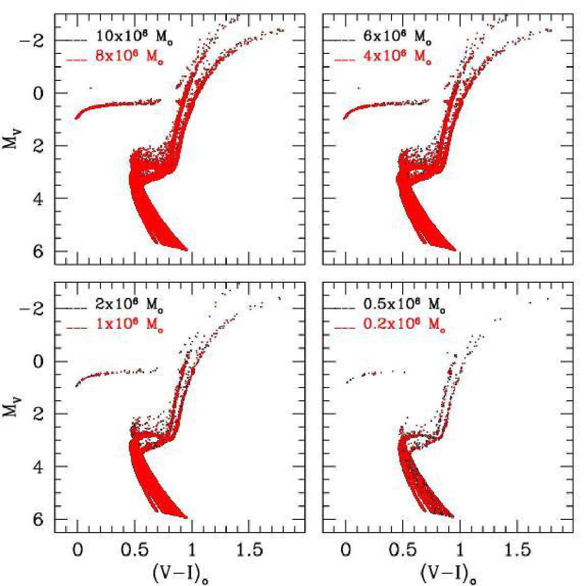 Figure 9
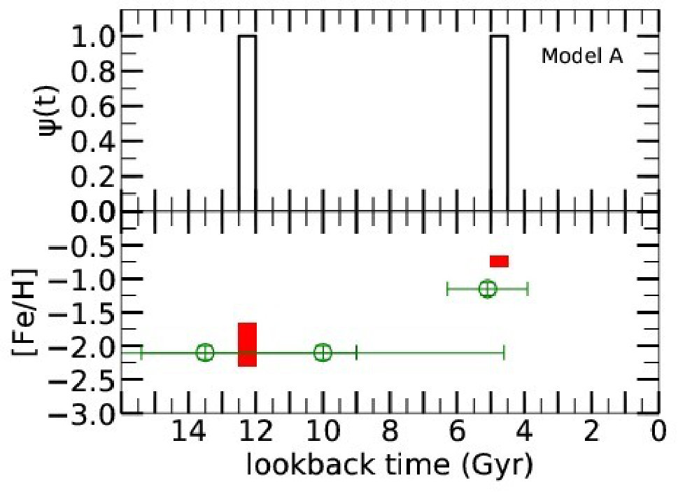 Figure 9
 Figure 10
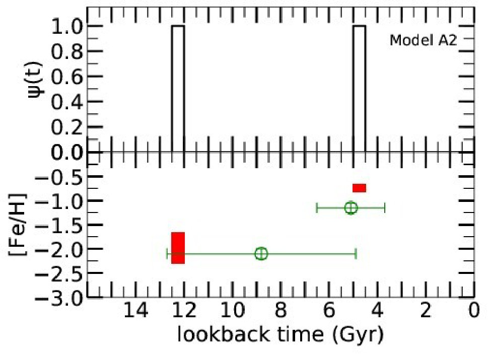 Figure 11
 Figure 12
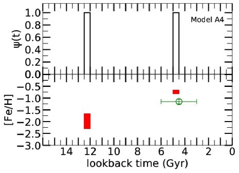 Figure 13
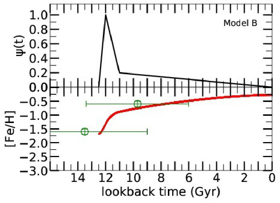 Figure 14
 Figure 15
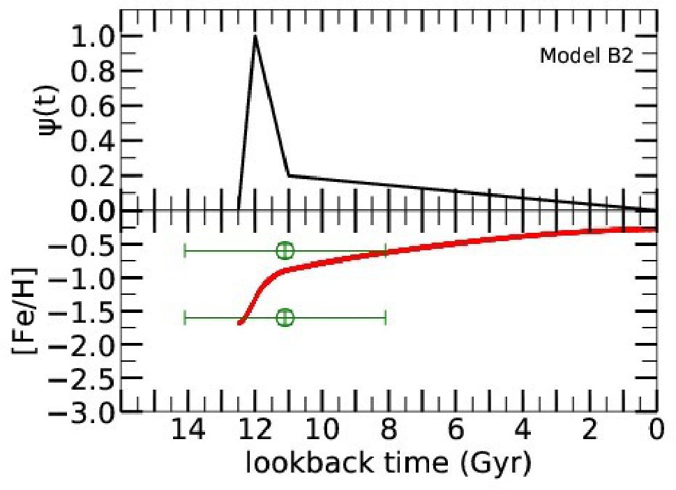 Figure 16
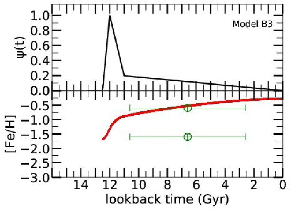 Figure 17
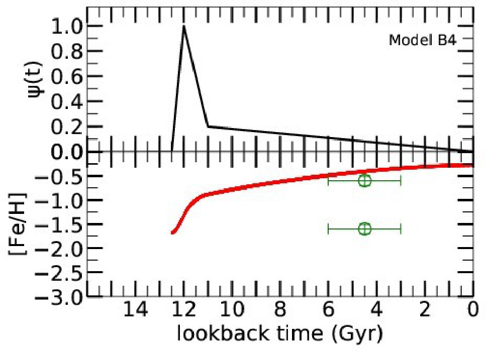 Figure 18
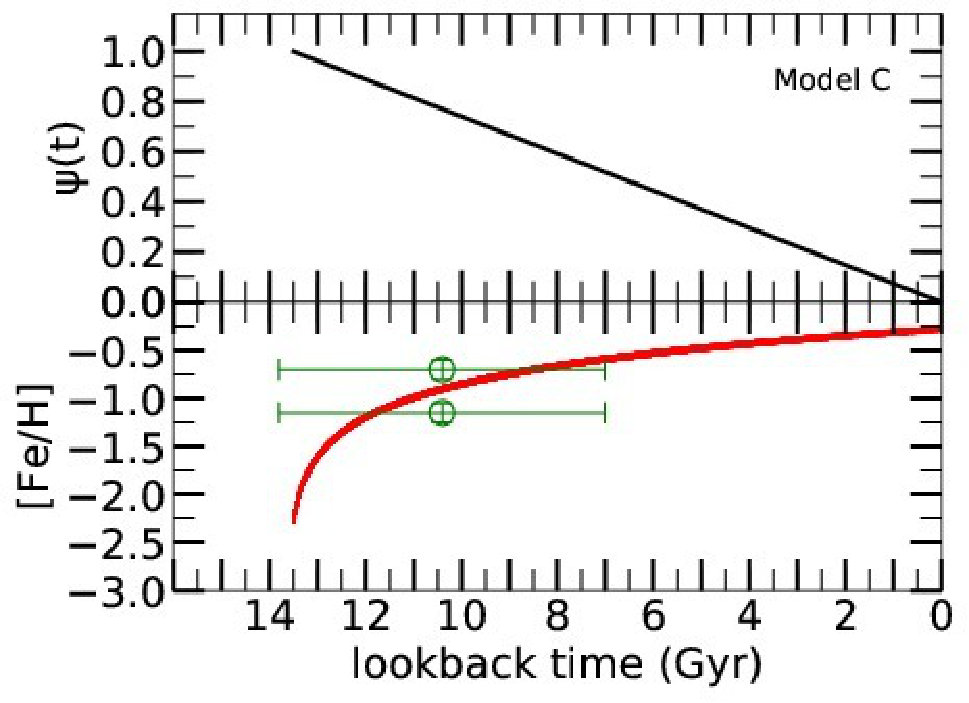 Figure 19
 Figure 20
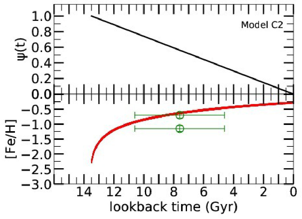 Figure 21
 Figure 22
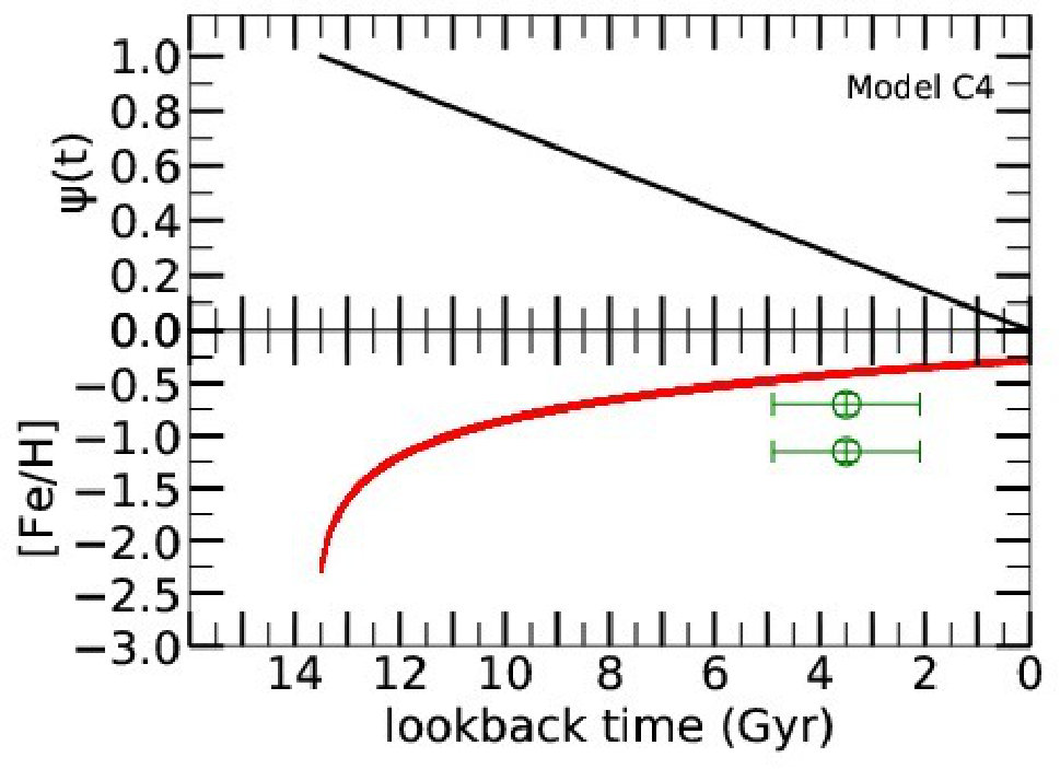 Figure 23
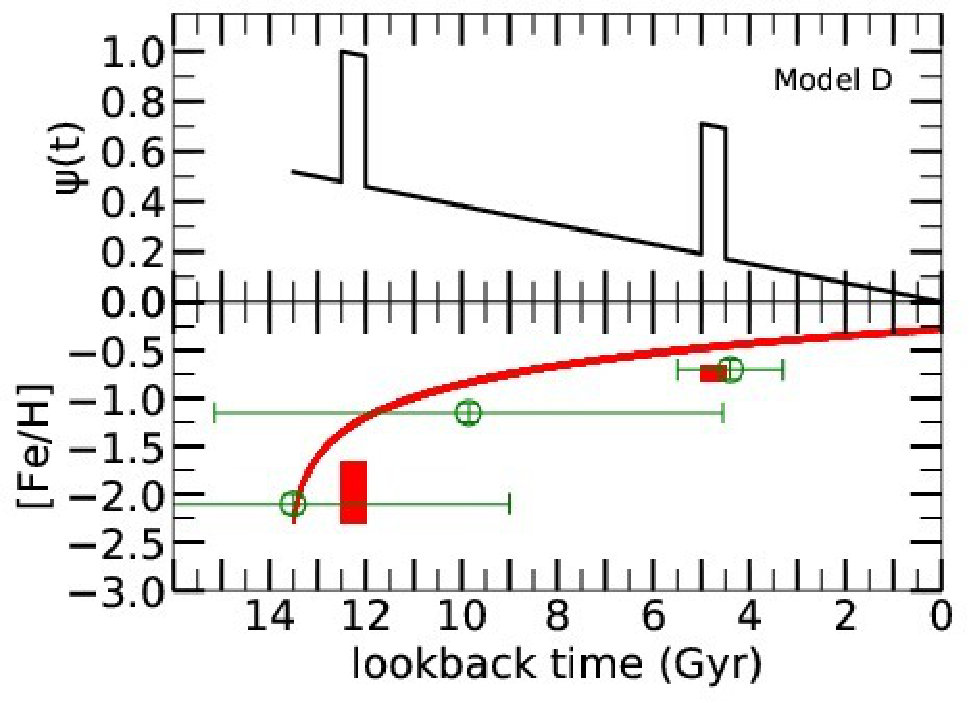 Figure 24
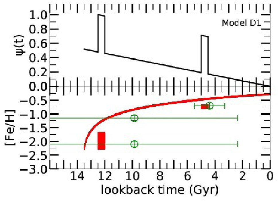 Figure 25
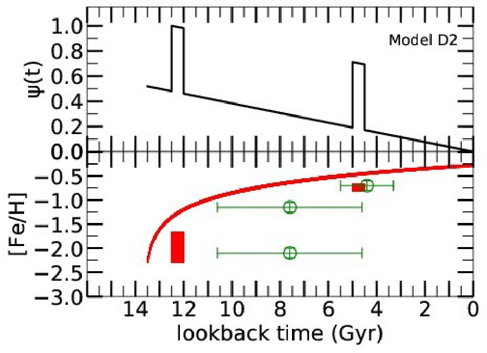 Figure 26
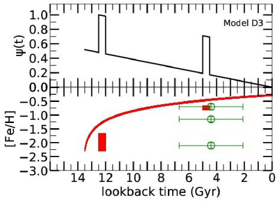 Figure 27
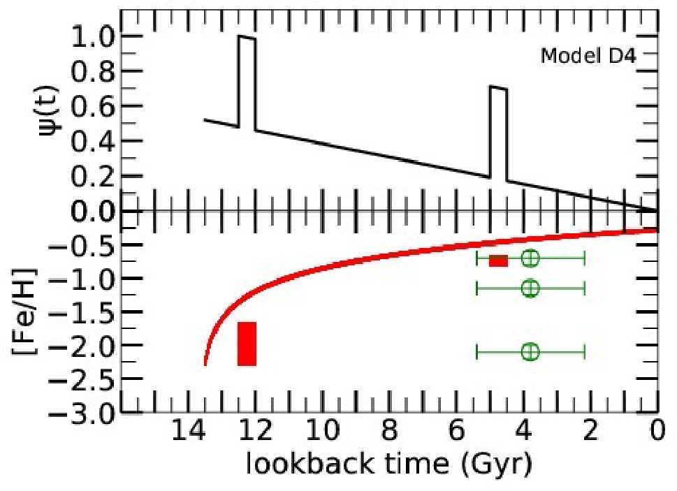 Figure 28
 Figure 29
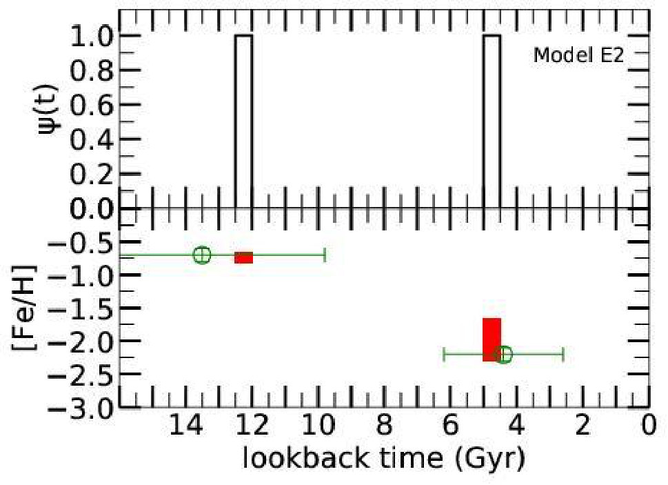 Figure 30
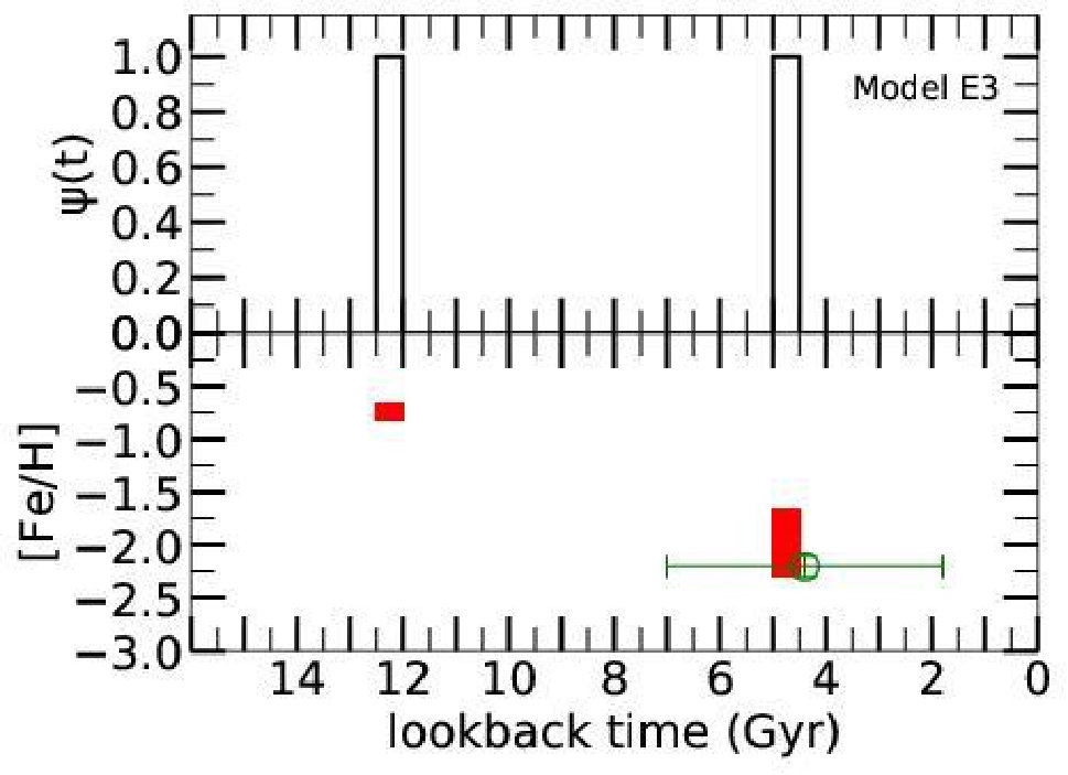 Figure 31
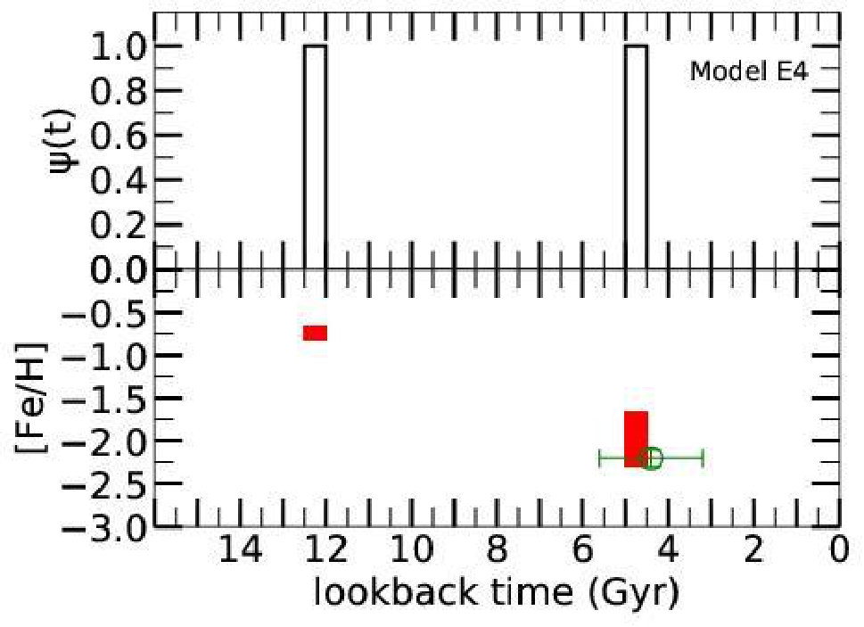 Figure 32
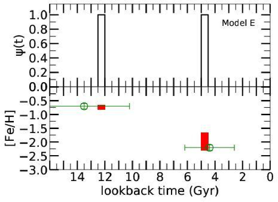 Figure 33
| Model | (TO) | (RC) | age | [Fe/H] | |
|---|---|---|---|---|---|
| (mag) | (mag) | (Gyr) | (mag) | (dex) | |
| A | 2.8750.200 | 0.4500.020 | 5.11.2 | 1.350.02 | 1.150.1 |
| 3.5000.500 | 0.4500.020 | 10.05.4 | 1.150.02 | 2.10.1 | |
| 4.8750.400 | 0.4500.020 | 13.5a | 1.150.02 | 2.10.1 | |
| A1 | 2.8750.200 | 0.4500.020 | 5.11.2 | 1.350.02 | 1.150.1 |
| 3.3750.400 | 0.4500.020 | 8.83.9 | 1.150.02 | 2.10.1 | |
| A2 | 2.8750.250 | 0.4500.020 | 5.11.4 | 1.350.02 | 1.150.1 |
| 3.3750.300 | 0.4500.020 | 8.83.9 | 1.150.02 | 2.10.1 | |
| A3 | 2.8750.250 | 0.4500.020 | 5.11.4 | 1.350.02 | 1.150.1 |
| A4 | 2.7500.300 | 0.4500.020 | 4.51.5 | 1.350.02 | 1.150.1 |
| B | 3.6250.350 | 0.6000.020 | 9.73.7 | 1.550.02 | 0.60.1 |
| 4.8750.300 | 0.6000.020 | 13.5a | 1.250.02 | 1.60.1 | |
| B1 | 3.7500.600 | 0.6000.020 | 11.16.0 | 1.550.02 | 0.60.1 |
| 3.7500.600 | 0.6000.020 | 11.16.0 | 1.250.02 | 1.60.1 | |
| B2 | 3.7500.300 | 0.6000.020 | 11.13.0 | 1.550.02 | 0.60.1 |
| 3.7500.300 | 0.6000.020 | 11.13.0 | 1.250.02 | 1.60.1 | |
| B3 | 3.2500.450 | 0.6000.020 | 6.64.0 | 1.550.02 | 0.60.1 |
| 3.2500.450 | 0.6000.020 | 6.64.0 | 1.250.02 | 1.60.1 | |
| B4 | 2.8750.300 | 0.6000.020 | 4.51.5 | 1.550.02 | 0.60.1 |
| 2.8750.300 | 0.6000.020 | 4.51.5 | 1.250.02 | 1.60.1 | |
| C | 3.6750.300 | 0.5900.020 | 10.43.4 | 1.500.02 | 0.70.1 |
| 3.6750.300 | 0.5900.020 | 10.43.4 | 1.350.02 | 1.150.1 | |
| C1 | 3.6750.450 | 0.5900.020 | 10.45.0 | 1.500.02 | 0.70.1 |
| 3.6750.450 | 0.5900.020 | 10.45.0 | 1.350.02 | 1.150.1 | |
| C2 | 3.3750.300 | 0.5900.020 | 7.63.0 | 1.500.02 | 0.70.1 |
| 3.3750.300 | 0.5900.020 | 7.63.0 | 1.350.02 | 1.150.1 | |
| C3 | 3.3750.400 | 0.5900.020 | 7.63.5 | 1.500.02 | 0.70.1 |
| 3.3750.400 | 0.5900.020 | 7.63.5 | 1.350.02 | 1.150.1 | |
| C4 | 2.6750.350 | 0.5900.020 | 3.51.4 | 1.500.02 | 0.70.1 |
| 2.6750.350 | 0.5900.020 | 3.51.4 | 1.350.02 | 1.150.1 | |
| D | 2.8750.200 | 0.5900.020 | 4.41.1 | 1.500.02 | 0.70.1 |
| 3.6250.500 | 0.5900.020 | 9.855.3 | 1.350.02 | 1.150.1 | |
| 4.8750.400 | 0.5900.020 | 13.5a | 1.150.02 | 2.10.1 | |
| D1 | 2.8750.200 | 0.5900.020 | 4.41.1 | 1.500.02 | 0.70.1 |
| 3.6250.700 | 0.5900.020 | 9.857.5 | 1.350.02 | 1.150.1 | |
| 3.6250.700 | 0.5900.020 | 9.857.5 | 1.150.02 | 2.10.1 | |
| D2 | 2.8750.200 | 0.5900.020 | 4.41.1 | 1.500.02 | 0.70.1 |
| 3.3750.350 | 0.5900.020 | 7.63.0 | 1.350.02 | 1.150.1 | |
| 3.3750.350 | 0.5900.020 | 7.63.0 | 1.150.02 | 2.10.1 | |
| D3 | 2.8750.450 | 0.5900.020 | 4.42.3 | 1.500.02 | 0.70.1 |
| 2.8750.450 | 0.5900.020 | 4.42.3 | 1.350.02 | 1.150.1 | |
| 2.8750.450 | 0.5900.020 | 4.42.3 | 1.150.02 | 2.10.1 | |
| D4 | 2.7500.350 | 0.5900.020 | 3.81.6 | 1.500.02 | 0.70.1 |
| 2.7500.350 | 0.5900.020 | 3.81.6 | 1.350.02 | 1.150.1 | |
| 2.7500.350 | 0.5900.020 | 3.81.6 | 1.150.02 | 2.10.1 | |
| E | 2.5000.250 | 0.2000.020 | 4.41.8 | 1.500.02 | 0.70.1 |
| 3.7500.200 | 0.2000.020 | 13.53.3 | 1.100.02 | 2.20.1 | |
| E1 | 2.5000.300 | 0.2000.020 | 4.41.6 | 1.500.02 | 0.70.1 |
| 3.7500.250 | 0.2000.020 | 13.54.0 | 1.100.02 | 2.20.1 | |
| E2 | 2.5000.350 | 0.2000.020 | 4.41.8 | 1.500.02 | 0.70.1 |
| 3.6250.250 | 0.2000.020 | 13.53.7 | 1.100.02 | 2.20.1 | |
| E3 | 2.5000.500 | 0.2000.020 | 4.42.6 | 1.500.02 | 0.70.1 |
| E4 | 2.5000.250 | 0.2000.020 | 4.41.2 | 1.500.02 | 0.70.1 |
Peer Reviews
No public reviews on file for this paper yet. If you reviewed it on a platform where reviews are public (OpenReview, ICLR, NeurIPS, ICML), you can paste yours below so the community can read it here.
Videos
No videos yet. Explain this paper in a talk, walkthrough, or lecture? Add one.
Representative galaxy age-metallicity relationships
Andrés E. Piatti1,2, Antonio Aparicio3,4 and Sebastián L. Hidalgo3,4
1Consejo Nacional de Investigaciones Científicas y Técnicas, Av. Rivadavia 1917, C1033AAJ, Buenos Aires, Argentina
2Observatorio Astronómico, Universidad Nacional de Córdoba, Laprida 854, 5000, Córdoba, Argentina
3Instituto de Astrofísica de Canarias, Calle Vía Láctea s/n, E-38200 La Laguna, Tenerife, Spain
4Departamento de Astrofísica, Universidad de La Laguna, Avda. Astrofísico Fco. Sánchez s/n, E-38206 La Laguna, Tenerife, Spain E-mail: [email protected] (AEP)
(Accepted XXX. Received YYY; in original form ZZZ)
Abstract
The ongoing surveys of galaxies and those for the next generation of telescopes will demand the execution of high-CPU consuming machine codes for recovering detailed star formation histories (SFHs) and hence age-metallicity relationships (AMRs). We present here an expeditive method which provides quick-look AMRs on the basis of representative ages and metallicities obtained from colour-magnitude diagram (CMD) analyses. We have tested its perfomance by generating synthetic CMDs for a wide variety of galaxy SFHs. The representative AMRs turn out to be reliable down to a magnitude limit with a photometric completeness factor higher than 85 per cent, and trace the chemical evolution history for any stellar population (represented by a mean age and an intrinsic age spread) with a total mass within 40 per cent of the more massive stellar population in the galaxy.
keywords:
techniques: photometric – galaxies:
††pubyear: 2016††pagerange: Representative galaxy age-metallicity relationships–Representative galaxy age-metallicity relationships
1 Introduction
The age-metallicity relationship (AMR) has fruitfully been employed to study the chemical evolution of different galactic and extragalactic stellar systems (e.g. Cohen, 1982; Catelan & de Freitas Pacheco, 1992; Rey et al., 2004). When dealing with the composed stellar population of a galaxy it has frequently been obtained from the galaxy star formation history (SFH) (e.g. Aparicio & Hidalgo, 2009; Hidalgo et al., 2011; de Boer et al., 2012; Savino et al., 2015). If such SFHs are extracted from synthetic colour-magnitude diagram-based tecniques (e.g. Sabbi et al., 2009; VandenBerg et al., 2015), they usually demand the consumption of a lot of CPU-time.
In order to be more expeditive in obtaining AMRs from large photometric databases, Piatti et al. (2012) developed a procedure based on the so-called representative stellar populations. The method has proved to be useful in comprehensively tracing the AMRs of the Large and Small Magellanic Clouds (L/SMC) (Piatti, 2012; Piatti & Geisler, 2013) and that of the Fornax spheroidal dwarf galaxy (Piatti et al., 2014) as well. In this work, we explore the advantages and constraints of such method in obtained astrophysically meaningful AMRs in a more general framework, by applying it to synthetic photometric data sets generated for a wide variety of galaxy SFHs.
In Section 2 we describe the procedure of building galaxy AMRs from their representative stellar populations and compare previous results from this method with those obtained from independent ones. In Section 3 we present different synthetic SFHs used to probe the ability of the aforementioned technique, while in Section 4 we analyze and discuss its usefulness in different galaxy formation and evolution scenarios.
2 The representative stellar populations method
Given the CMD of a composed stellar population, Piatti et al. (2012) assumed that the observed main sequence (MS) in any galaxy field is a result of the superposition of MSs with different turnoffs (TOs) and constant luminosity functions (LFs). Hence, the difference between the number of stars of two adjacent magnitude intervals gives the intrinsic number of stars belonging to the faintest interval. Consequently, the biggest difference is directly related to the most populated TO. Geisler et al. (2003) defined this TO as representative of a comparatively small field in the sky along the line of sight, and soon after was used by Piatti et al. (2003a, b, 2007), among others, for revealing the primary trends of the stellar composition in different galaxy fields in an efficient and robust way. The definition of a representative TO could not converge to any dominant TO (age) value if the stars in a given field came from a constant star formation rate (SFR) integrated over all time. In such a case, the difference between the number of stars of two adjacent magnitude intervals would result in the same value for any magnitude interval.
The concept of representative TOs is directly applied to AMRs whenever the ages and metallicities used to build them come from representative values, i.e., ages and metallicities estimated by using the photometric information of the prevailing stellar populations. These prevailing populations trace the present-day AMR of a galaxy. They account for the most important metallicity-enrichment processes that have undergone in the galaxy lifetime. Minority stellar populations not following these main chemical galactic processes are discarded. Therefore, presently-subdominant populations in certain locations could have been present in the majority in the galaxy in the past, but were not considered. Note that any AMR built from representative ages and metallicities differs from those derived from modelled SFHs in the fact that it does not include complete information on all stellar populations, but accounts for the dominant population present in each field.
Red clumps (RCs) stars are usually used as standard candles for distance determinations (Paczyński & Stanek, 1998; Olsen & Salyk, 2002; Subramaniam, 2003). However, they are also often used in age estimates based on the magnitude difference between the HB/clump and the MSTO for intermediate-age and old clusters (see, e.g. Phelps et al., 1994), since the RC mag is relatively invariant to population effects such as age and metallicity for such stars (Girardi & Salaris, 2001). Since the MSTO magnitude is an excellent age indicator, so also is the difference (in magnitude) MSTO RC. By assuming that the peak of the RC magnitude distribution of a composed stellar population corresponds to the most populous MSTO in the respective field, it is possible to estimate representative ages from composed stellar population CMDs, particularly for ages older than 1 Gyr. For younger ages the magnitude of the He-burning stage varies with age for such massive stars. Note that this age measurement technique does not require absolute photometry and is independent of reddening and distance as well. An additional advantage is that it is not needed to go deep enough to see the extended MS of the representative stellar population but only slightly beyond its MSTO.
As for the representative metallicities, they can be derived following similar precepts, i.e., by identifying the prevailing stellar population (the more numerous one) in the CMD or Hess diagram of a particular field. For instance, if the position, slope and/or shape of the red giant branch (RGB) is used as a metallicity indicator (e.g. Da Costa & Armandroff, 1990; Geisler & Sarajedini, 1999; Valenti et al., 2004; Choudhury et al., 2016), the fiducial placement of the densest RGB path should be considered. Depending on the metallicity sensitivity of the photometric system, particular caveats should be taken into account for those photometric metallicity estimation methods that show some slight dependence with age (Geisler et al., 2003; Ordoñez & Sarajedini, 2015).
Piatti (2012) and Piatti & Geisler (2013) built representative AMRs for the SMC and LMC using some 3.3 and 5.5 million stars observed in the Washington photometric system, respectively, distributed throughout the main body of each galaxy. The representative MSTO magnitudes turned out to be on average 0.6 mag brighter than the mag for the 100% completeness level of the respective fields, so that they actually reached the TO of the representative population of each field. Fig. 1 reproduces their AMRs that trace the main features of the chemical enrichment experienced by these galaxies. Since them, some other independent AMRs have been obtained by Rubele et al. (2012, survey) and Bekki & Tsujimoto (2012, theoretical model) for the LMC, and by Cignoni et al. (2013, photometry) and Rubele et al. (2015, survey) for the SMC, among others. Particularly, Rubele et al. (2012, 2015) and Cignoni et al. (2013) used independent procedures to fit synthetic CMDs to the data. They have been overplotted on Fig. 1 for comparison purposes. As can be seen, all of them agree reasonably well.
Piatti et al. (2014) applied also the representative stellar population method to study the AMR of the Fornax dwarf spheroidal galaxy from photometric data obtained with FORS1 at the VLT. According to del Pino et al. (2013), the derived representative (MSTO) mags of each surveyed subregion are brighter than the mag at the 90% completeness level, so that they actually reached the MSTO of the representative oldest populations of the galaxy, particularly in those regions where the oldest populations are indeed the dominant population. When focusing on the most prominent stellar populations, they found that the derived AMRs are engraved by the evidence of an outside-in star formation process and suggested for the first time a possible merger of two galaxies that would have triggered a star formation bursting process that peaked between 6 and 9 Gyr ago, depending on the position of the field in the galaxy. Later on, other studies showed similar outcomes (Hendricks et al., 2014; del Pino et al., 2015; Wang et al., 2016), thus validating the representative stellar population method.
At this point a question arises unavoidably: since the concept representative has associated a specific galaxy tracer (the representative stellar population), we wonder whether there are scenarios in the galaxy formation and evolution for which the representative tracer differs from considering as tracers the whole stellar populations. In other words, could the representive AMR be used to describe the global chemical enrichment history of any galaxy? In the subsequent Section we thoroughly examine its scope and constraints.
3 synthetic age-metallicity relationships
3.1 The models
In order to test wether the representative AMRs are robust representations of the most significant age and metallicity present in CMDs we have carried out the following procedure. First, we have generated four synthetic stellar populations with different input SFRs and AMRs; second, we have simulated realistic observational effects in their CMDs, and finally, we have applied the representative AMR method to each of the synthetic CMDs. Comparison of the obtained results and the input data will provide the required information for the robustness test. A short description of the first and second steps follows.
We have used IAC-star (Aparicio & Gallart, 2004) to compute the four synthetic stellar populations. They have been labeled as A, B, C, D and E and their SFRs and AMRs are shown in Figs. 2 to 6. The characteristics of the populations are as follows: population A consists in two bursts lasting 0.5 Gyr each and starting at ages 12.5 and 5 Gyr, respectively. A metallicity dispersion is used for each one: for the old one and for the young one. Population B begins with a burst that starts at 12.5 Gyr in age, peaks at 12 Gyr and goes down to a low rate at 11 Gyr; after that, the star formation is low and goes on mildly decreasing to 0 at present. The metallicity follows a closed box model with initial value , final value and final gas mass fraction ; to this, a gaussian dispersion has been added such that . Population C starts at age 13.5 Gyr with a high SFR that decreases linearly to 0 at present. The metallicity increases linearly from an initial value of to a final value of . As in the former case, a gaussian metallicity dispersion has been added such that . Finally, population D is simply the sum of populations A and C. In all the cases, a double power law has been assumed for the Initial Mass Function with exponent for the stellar mass interval M⊙ and for the interval M⊙. Also, a fraction of 30% binary stars has been assumed, with a flat secondary to primary mass ratio distribution with minimum value 0.5 and maximum, 1. The number of stars in the vs. CMD, down to a magnitude limit of , has been fixed in stars for models A, B and C and stars for model D. These figures translate in ever formed star masses of M⊙ for models A, B and C and M⊙ for model D.
Regarding observational effects, four scenarios have been simulated in each population. The corresponding CMDs are labeled from 1 to 4 for each synthetic population; e.g. A1, A2, A3, and A4, for the case of population A. Each scenario is represented by a completeness function and an error distribution. In Fig. 7, completeness as a function of (upper panel) and errors as a function of and (bottom panel) are plotted for the four scenarios. Completeness is simulated in the following way: for each star, the completeness fraction corresponding to its magnitude is obtained. Then a random number generator is used to maintain or eliminate the star from the photometry list; the star is conserved if the random number is smaller than the completeness fraction. Errors are simulated in the following way: for each conserved star, shifts in magnitudes in both filters are applied randomly selected from gaussian distributions which standard deviations are the values of (plotted in Fig. 7) and , respectively. In order to illustrate the reader, Fig. 8 depicts some of the generated synthetic CMDs.
3.2 Representative AMRs
Fig. 9 illustrates, as an example, the generated vs CMD for model B, which includes 100,000 stars. A mixture of young through old stellar populations clearly appears to be the main feature of this CMD. Other obvious traits presented in the CMD are the populous and broad subgiant branches (an indicator of the evolution of stars with ages (masses) within a non-negligible range), the RCs and the RGBs. In the middle panel of Fig. 9 we drew the respective MS LF. The whole set of MS LFs (one for each model) were obtained by counting the number of stars in bins of 0.25 mag along the MSs, and then they were normalized. The chosen bin size encompasses typical magnitude errors of the stars in each bin, thus producing an appropriate sample of the stars. Note that accurate photometries have magnitude errors for most of the measured stars usually smaller than 0.20 mag. As is well-known, the bin size should be of the order of the uncertainties of the quantity involved to best represent an intrinsic distribution of such a quantity (Piatti, 2010, 2011). This means statistically speaking that the shape of these LFs are not driven by the chosen bin size.
We then computed for each synthetic CMD the difference between the number of stars of two adjacent magnitude intervals to produce the differential MS LF, as illustrated in the right panel of Fig. 9. As described in Section 2, the peak and the broadness of the differential MS LF provide information about the representative TO magnitude and its intrinsic width of the considered stellar populations. The prevailing TO (differential MS LF peak) of each synthetic CMD resulted typically more populous than the next most dominant population, represented by a secondary peak sometimes there even could exist a third peak in the differential LFs. We adopted here the two main peaks we distinguished in the differential MS LFs, as well as their observed FWHMs, as a measure of their intrinsic broadnesses. For the synthetic CMDs of models A, D, D1, D2, D3 and D4 we distinguished three main peaks, whereas for those of models A3 and A4 only one peak. Table 1 lists the representative (TO) with their associated widths for each modelled SFH.
As for the representative RCs, we built distributions for the RC stars and performed gaussian fits to derive the mean values and the FWHMs. We performed gaussian fits using the ngaussfit routine of the IRAF111IRAF is distributed by the National Optical Astronomy Observatories, which is operated by the Association of Universities for Research in Astronomy, Inc., under contract with the National Science Foundation. stsdas package. We adopted a single gaussian, and fixed the constant and linear terms to the corresponding background levels and to zero, respectively. The centre of the gaussian, its amplitude, and its FWHM acted as variables. Table 1 lists the resulting representative (RC).
Since we are primarily interested in determining the age and metallicity of the representative star population in each model, we derived indices by calculating the difference in the magnitude between the RC and the MSTO. We then derived ages from the values by using the equation (Piatti et al., 2014):
[TABLE]
This equation is only calibrated for ages larger than 1 Gyr, so that we are not able to produce ages for younger representative populations. Table 1 presents the resultant ages and their dispersions. The dispersions have been calculated bearing in mind the broadness of the mag distributions of the representative MSTOs and RCs, and represent in general a satisfactory estimate of the age spread around the prevailing population age.
In addition, we also estimated representative metallicities using the equation:
[TABLE]
of Da Costa & Armandroff (1990), once the colours of the RGB at = 3.0 mag and their dispersions were obtained. The colours were derived from the intersection of the RGBs traced for each model and the horizontal line at = 3.0 mag. Table 1 provides with the resulting values and the derived representative metallicities.
4 Discussion and Conclusions
In the bottom panels of Figures 2 to 6 we superimposed the representative ages and metallicities derived in Sect. 3.2 (green open boxes) to the modelled AMRs (red lines). The errorbars represent the intrinsic FWHMs of such representative values. In this Section we compare the trends suggested by the representative age/metallicity values with those coming directly from the modelled SFHs. In other words, we assess how well main changes in the modelled AMRs are detected by the representative AMRs. Note that the representative method is not meant to reproduce any particular modelled stellar population, but to map the main trends in the present-day AMR from the so-called representative populations.
At first glance, there are clear differences in the success with which the representative AMRs represent the actual AMR. For instance, completeness effects constrain significantly the performance of representative AMRs, a result which is expected since representative AMRs come from the employment of observed CMDs with different completeness effects. From the inspection of Figures 2 to 6 we found that the oldest representative age is highly dependent on this completeness factor. As can be seen, the lower the photometry completeness the younger the oldest representative age derived. They are in agreement (considering their errorbars) with the oldest modelled ages only for models without completeness effect (models A, B, C, D and E) and models with completeness effect # 1 and 2, and in some few cases # 3. Thus, by entering into Fig. 7 with the absolute magnitude associated to the MSTO of these oldest representative ages (see Table 1) we found that the associated completeness factor is higher than 85 per cent. This means that reliable oldest representative ages can be obtained for stellar populations with a photometry completeness higher than 85 per cent. Dominant stellar populations observed with less complete photometry do not come up as representative ones. This is somehow an expected result, since it would be hardly possible to say anything about a prevailing stellar population if it were not observed mostly complete. Indeed, the representative AMRs built by Piatti (2012); Piatti & Geisler (2013) and Piatti et al. (2014) for the SMC, LMC and the Fornax dwarf spheroidal, respectively, were obtained from photometry with completeness factors higher than 90 per cent, and hence the good agreement seen with other independent AMRs.
As for the metallicities, we found that the representative AMRs were able to reasonably account for the modelled metallicity enrichment ranges when they arose as a consequence of a bursting formation event (models A, B, D and E). Particularly, the metal-poor ends were mostly well reproduced, while the metal-rich one resulted 0.3–0.4 dex more metal-poor. The latter could be due to a relatively low metallicity sensitivity of the employed photometric system toward the metal-rich end. This does not happen, for instance, for the Washington photometric system which is more sensitive to metallicity (see. Fig. 1). Likewise, the modelled age ranges were more satisfactorily reproduced by the resulting representative age ranges whenever models contained bursting formation events.
During quiescent periods of star formation or periods with a decreasing SFR, as is the case of model C, the representative AMRs provide only with mean values of age and metallicity for all the stars formed at (t) higher than 0.6. This can be easily checked by entering into Fig. 4 with the representative ages (mean values and errors) and interpolate the (t) one for model C (without completeness effect). This means that detected representative populations consist of any stellar population whose stars are within at least 40 per cent of the most massive one in the galaxy. As we mention in Sect. 2, the definition of a representative TO – and hence of a representative stellar population – could not converge to any dominant TO (age) value if the stars in a given field came from a constant star formation rate (SFR) integrated over all time. Likewise, minority stellar populations not following these main chemical galactic processes are discarded. Both nearly constant SFR and minority population effects can be seen in Fig. 3 to 6 (models B, C, D and E), where only main bursts were detected.
On the other hand, we confirm that the representative method is suitable to detect mayor star formation events in the galaxy lifetime, such as bursts of stellar populations. For instance, bursts in models A (at 5 and 12 Gyr), B (at 12 Gyr), D (at 5 and 12 Gyr) and E (at 5 and 12 Gyr) are well detected, provided a good photometric completeness. This is because a mayor bursting event can produce a significant amount of stars (not necessarily followed by a chemical enrichment), and therefore representative populations during the galaxy lifetime can emerge. Moreover, even though the B, C and D modelled AMRs are similar – they consist of an important increase in the metallicity at the very begining of the galaxy formation and nearly flat curves with a small slope around [Fe/H] 0.5 dex over most of the galaxy lifetime – the representative AMRs resulted different because of the differences in the SFHs. Those representative AMRs obtained from models with bursting stellar formation events reproduced better the age/metallicty modelled ranges. Successive bursts of star formation could be recognized if the conditions mentioned above about the completeness factor and the (t) value are fulfilled.
Recovering the dominant stellar population(s), and hence the representative AMRs, depends on the total mass of the galaxy. This is because a representative AMR relies on the composite CMD of the galaxy stellar populations. If real representative MSTOs, RCs or RGBs are not visible in the CMD, the method cannot be employed. To illustrate this point we generated synthetic stellar populations (synthetic CMDs) with different input total masses for our model A. The resulting synthetic CMDs are shown in Fig. 10. As can be seen, below 1-2106 M⊙, the redder RGB and the brighter MSTO are difficult to recognize. We then derived representative ages and metallicities for each model and drew Fig. 11 which compares the different outcomes. Once again, the originally modelled AMR (model A) is not recovered for galaxy masses smaller than 1-2106 M⊙. For galaxy masses smaller than 0.5106 M⊙, the RGB was not detected, so that we could not estimate representative metallicities.
The ongoing surveys of galaxies, e.g., Kelson et al. (2014, CSI), Calzetti et al. (2015, LEGUS) and those for the next generation of telescopes will demand plenty of CPU time to recover a detailed galaxy SFH. This challenge points to the need of expeditive methods for obtaining quick-look AMRs before high-CPU consuming machine codes can be fully executed. The representative method presented here could be of a great help in this respect, providing AMRs in advance (nearly in real time respect to the availability of observational data) which statistically reflect the most important trends in the galaxy formation and chemical evolution. The representative AMRs turn out to be reliable down to a magnitude limit with a photometric completeness factor higher than 85 per cent, and trace the chemical evolution history for any stellar population (represented by a mean age and an intrinsic age spread) with a total mass within 40 per cent of the most massive stellar population in the galaxy.
Acknowledgements
We thank the referee, Jacco van Loon, for his thorough reading of the manuscript and timely suggestions to improve it.
The reference list from the paper itself. Each links out to its DOI / PubMed record.
- 1Aparicio & Gallart (2004) Aparicio A., Gallart C., 2004, AJ , 128, 1465 · doi ↗
- 2Aparicio & Hidalgo (2009) Aparicio A., Hidalgo S. L., 2009, AJ , 138, 558 · doi ↗
- 3Bekki & Tsujimoto (2012) Bekki K., Tsujimoto T., 2012, Ap J , 761, 180 · doi ↗
- 4Calzetti et al. (2015) Calzetti D., et al., 2015, AJ , 149, 51 · doi ↗
- 5Catelan & de Freitas Pacheco (1992) Catelan M., de Freitas Pacheco J. A., 1992, A&A, 258, L 5
- 6Choudhury et al. (2016) Choudhury S., Subramaniam A., Cole A. A., 2016, MNRAS , 455, 1855 · doi ↗
- 7Cignoni et al. (2013) Cignoni M., Cole A. A., Tosi M., Gallagher J. S., Sabbi E., Anderson J., Grebel E. K., Nota A., 2013, Ap J , 775, 83 · doi ↗
- 8Cohen (1982) Cohen J. G., 1982, Ap J , 258, 143 · doi ↗