Reinforcement Learning Based Dynamic Selection of Auxiliary Objectives with Preserving of the Best Found Solution
Irina Petrova, Arina Buzdalova

TL;DR
This paper introduces a reinforcement learning-based method for dynamically selecting auxiliary objectives in optimization, effectively preserving the best solutions and outperforming existing approaches across multiple problems.
Contribution
It proposes a novel modification of the EA+RL method that prevents losing the best solution during auxiliary objective selection, with theoretical and empirical validation.
Findings
Outperforms EA+RL on all tested problems.
Surpasses single-objective approach on most instances.
Provides detailed analysis of algorithm components' influence.
Abstract
Efficiency of single-objective optimization can be improved by introducing some auxiliary objectives. Ideally, auxiliary objectives should be helpful. However, in practice, objectives may be efficient on some optimization stages but obstructive on others. In this paper we propose a modification of the EA+RL method which dynamically selects optimized objectives using reinforcement learning. The proposed modification prevents from losing the best found solution. We analysed the proposed modification and compared it with the EA+RL method and Random Local Search on XdivK, Generalized OneMax and LeadingOnes problems. The proposed modification outperforms the EA+RL method on all problem instances. It also outperforms the single objective approach on the most problem instances. We also provide detailed analysis of how different components of the considered algorithms influence efficiency of…
Click any figure to enlarge with its caption.
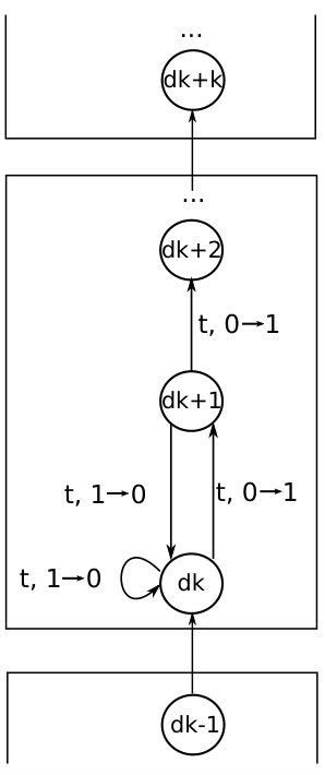 Figure 1
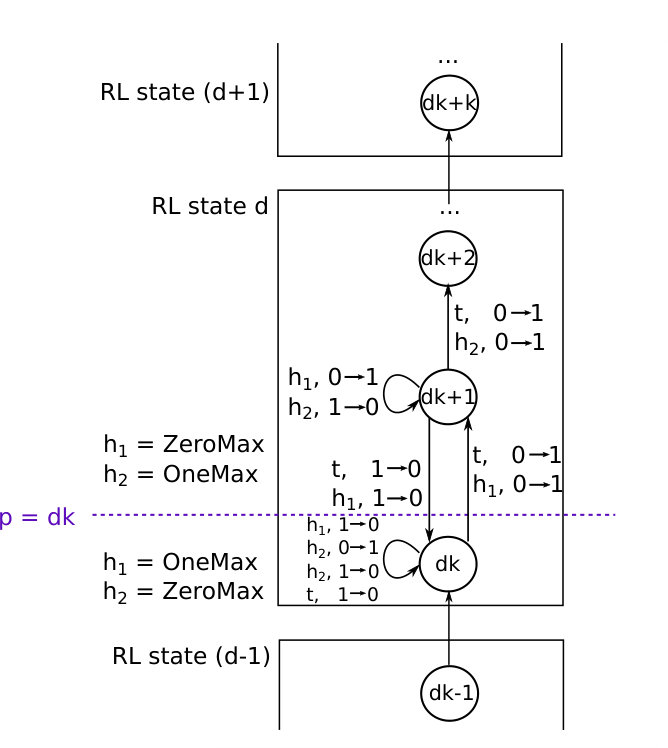 Figure 2
| modified EARL, learning | modified EARL, no learning | EARL | ||||||||
| Parameters | RLS | ss, | ts, | ts, | ss, | ts, | ts, | ss, | ts, | ts, |
| n | LeadingOnes | |||||||||
| 1 | 1.46 | 1.65 | 1.72 | 1.76 | 1.77 | 1.72 | 1.77 | inf | inf | inf |
| 11 | inf | inf | inf | |||||||
| 21 | inf | inf | inf | |||||||
| 31 | inf | inf | inf | |||||||
| 41 | inf | inf | inf | |||||||
| 51 | inf | inf | inf | |||||||
| 61 | inf | inf | inf | |||||||
| 71 | inf | inf | inf | |||||||
| 81 | inf | inf | inf | |||||||
| 91 | inf | inf | inf | |||||||
| 101 | inf | inf | inf | |||||||
| 111 | inf | inf | inf | |||||||
| 121 | inf | inf | inf | |||||||
| 131 | inf | inf | inf | |||||||
| 141 | inf | inf | inf | |||||||
| 151 | inf | inf | inf | |||||||
| 161 | inf | inf | inf | |||||||
| 171 | inf | inf | inf | |||||||
| 181 | inf | inf | inf | |||||||
| 191 | inf | inf | inf | |||||||
| n, d | OMd | |||||||||
| 100, 50 | ||||||||||
| 200, 100 | ||||||||||
| 300, 150 | ||||||||||
| 400, 200 | ||||||||||
| 500, 250 | ||||||||||
| n, k | XdivK, switch point in the end | |||||||||
| 40, 2 | inf | |||||||||
| 48, 2 | inf | |||||||||
| 56, 2 | inf | |||||||||
| 64, 2 | inf | |||||||||
| 72, 2 | inf | |||||||||
| 80, 2 | inf | |||||||||
| 60, 3 | inf | |||||||||
| 72, 3 | inf | |||||||||
| 84, 3 | inf | inf | ||||||||
| 96, 3 | inf | inf | ||||||||
| 108, 3 | inf | inf | ||||||||
| 120, 3 | inf | inf | ||||||||
| n, k | XdivK, switch point in the middle | |||||||||
| 40, 2 | inf | |||||||||
| 48, 2 | inf | |||||||||
| 56, 2 | inf | |||||||||
| 64, 2 | inf | |||||||||
| 72, 2 | inf | |||||||||
| 80, 2 | inf | |||||||||
| 60, 3 | inf | |||||||||
| 72, 3 | inf | |||||||||
| 84, 3 | inf | |||||||||
| 96, 3 | inf | inf | ||||||||
| 108, 3 | inf | inf | ||||||||
| 120, 3 | inf | inf | ||||||||
Peer Reviews
No public reviews on file for this paper yet. If you reviewed it on a platform where reviews are public (OpenReview, ICLR, NeurIPS, ICML), you can paste yours below so the community can read it here.
Videos
No videos yet. Explain this paper in a talk, walkthrough, or lecture? Add one.
Taxonomy
TopicsAdvanced Multi-Objective Optimization Algorithms · Evolutionary Algorithms and Applications · Metaheuristic Optimization Algorithms Research
Reinforcement Learning Based
Dynamic Selection of Auxiliary Objectives
with Preserving of the Best Found Solution
Irina Petrova, Arina Buzdalova
ITMO University
49 Kronverkskiy av.
Saint-Petersburg, Russia, 197101
Email: [email protected], [email protected]
Abstract
Efficiency of single-objective optimization can be improved by introducing some auxiliary objectives. Ideally, auxiliary objectives should be helpful. However, in practice, objectives may be efficient on some optimization stages but obstructive on others. In this paper we propose a modification of the EA+RL method which dynamically selects optimized objectives using reinforcement learning. The proposed modification prevents from losing the best found solution.
We analysed the proposed modification and compared it with the EA+RL method and Random Local Search on XdivK, Generalized OneMax and LeadingOnes problems. The proposed modification outperforms the EA+RL method on all problem instances. It also outperforms the single objective approach on the most problem instances. We also provide detailed analysis of how different components of the considered algorithms influence efficiency of optimization. In addition, we present theoretical analysis of the proposed modification on the XdivK problem.
I Introduction
Consider single-objective optimization of a target objective by an evolutionary algorithm (EA). Commonly, efficiency of EA is measured in one of two ways. In the first one efficiency is defined as the number of fitness function evaluations needed to reach the optimum. In the second one efficiency of EA is computed as the maximum target objective value obtained within the fixed number of evaluations. In this work we use the first way.
Efficiency of the target objective optimization can be increased by introducing some auxiliary objectives [1, 2, 3, 4, 5]. Ideally, auxiliary objectives should be helpful [2]. However, in practice, objectives can be generated automatically and may be efficient on some optimization stages but obstructive on others [6, 7]. We call such objectives non-stationary. One of the approaches to deal with such objectives is dynamic selection of the best objective at the current stage of optimization. The objectives may be selected randomly [8]. The better method is EA+RL which uses reinforcement learning (RL) [9, 10].
It was theoretically shown for a number of optimization problems that EA+RL efficiently works with stationary objectives [11, 12]. However, theoretical analysis of EA+RL with non-stationary objectives showed that EA+RL does not ignore obstructive objective on the XdivK problem [13]. Selection of an inefficient auxiliary objective causes losing of the best found solution and the algorithm needs a lot of steps to find a good solution again. Also EA+RL can stuck in local optima while solving the Generalized OneMax problem with obstructive objectives [14].
In this paper we propose a modified version of EA+RL and analyse it theoretically and experimentally on XdivK, Generalized OneMax and LeadingOnes problems. The rest of the paper is organized as follows. First, the EA+RL and model problems with non-stationary objectives are described. Second, a modification of the EA+RL method is proposed. Then we experimentally analyse the considered methods. Finally, we provide discussion and theoretical explanation of the achieved results.
II Preliminaries
In this section we describe the EA+RL method. Also we define model problems and non-stationary objectives used in this study.
II-A EA+RL method
In reinforcement learning (RL) an agent applies an action to an environment. Then the environment returns a numerical reward and a representation of its state and the process repeats. The goal of the agent is to maximize the total reward [9].
In the EA+RL method, EA is treated as an environment, selection of an objective to be optimized corresponds to an action. The agent selects an objective, EA generates new population using this objective and returns some reward to the agent. The reward depends on difference of the best target objective value in two subsequent generations. We consider maximization problems. So the higher is the newly obtained target value, the higher is the reward.
In recent theoretical analysis of EA+RL with non-stationary objectives, random local search (RLS) is used instead of EA, population consists of a single individual [13]. Individuals are represented as bit strings, flip-one-bit mutation is used. If values of the selected objective computed on the new individual and on the current one are equal, the new individual is accepted. The used reinforcement learning algorithm is Q-learning. Therefore, the EA+RL algorithm in this case is called RLS + Q-learning. The pseudocode of RLS + Q-learning is presented in Algorithm 1. The current state is defined as the target objective value of the current individual. The reward is calculated as difference of the target objective values in two subsequent generations. In Q-learning, the efficiency of selecting an objective in a state is measured by the value which is updated dynamically after each selection as shown in line 13 of the pseudocode, where and are the learning rate and the discount factor correspondingly.
II-B Model problems
In this paper we consider three model problems which were used in studies of EA+RL [13, 12, 14]. In all considered problems, an individual is a bit string of length . Let be the number of bits in an individual which are set to one. Then the objective OneMax is equal to and the objective ZeroMax is equal to .
One of the considered problems is Generalized OneMax, denoted as . The target objective of this problem called is calculated as the number of bits in an individual of length that matches a given bit mask. The bit mask has 0-bits and 1-bits.
Another problem is XdivK. The target objective is calculated as , where is the number of ones, is a constant, and divides .
The last considered problem is LeadingOnes. The target objective of this problem is equal to the length of the maximal prefix consisting of bits set to one.
II-C Non-stationary objectives
We used the two following non-stationary auxiliary objectives for all the considered problems. These auxiliary objectives can be both OneMax or ZeroMax at different stages of optimization. More precisely, consider the auxiliary objectives and defined in (1). The parameter is called a switch point, because at this point auxiliary objectives change their properties. OneMax and ZeroMax are denoted as OM and ZM correspondingly.
[TABLE]
In the XdivK problem, an objective which is currently equal to OneMax allows to distinguish individuals with the same value of the target objective and give preference to the individual with a higher value. Such an individual is more likely to produce a descendant with a higher target objective value. In the LeadingOnes problem, OneMax is helpful because it has the same optimum but running time of optimizing OneMax is lower [15]. Therefore, in LeadingOnes and XdivK problems the objective which is equal to OneMax at the current stage of optimization is helpful. In both these problems, the goal is to obtain individual of all ones, so ZeroMax is obstructive.
In the problem, both objectives may be obstructive or neutral. For example, if for some the -th bit of the bit mask is set to 1, and the mutation operator flips the -th bit of an individual from 0 to 1, the ZeroMax objective is obstructive, because it would not accept this individual. In the inverse case, OneMax is obstructive.
III Modified EA+RL
In this section we propose a modification of the EA+RL method which prevents EA+RL from losing the best found solution. In the EA+RL method, if the newly generated individual is better than the existing one according to the selected objective, the new individual is accepted. However, if the selected objective is obstructive, the new individual may be worse than the existing individual in terms of the target objective. In this case EA loses the individual with the best target objective value.
In the modified EA+RL, if the newly generated individual is better than the existing one according to the selected objective, but is worse according to the target objective, the new individual is rejected. As in the recent theoretical works, we use RLS as optimization problem solver and apply Q-learning to select objectives. The pseudocode of the modified RLS + Q-learning is presented in Algorithm 2.
To motivate the approach of reward calculation in the new method, we need to describe how the agent learns which objective should be selected in the EA+RL method. If the agent selects an obstructive objective and EA loses individual with the best target value, the best target value in the new generation is decreased. So the agent achieves a negative reward for this objective and will not select this objective in the same state later. However, when properties of auxiliary objectives are changed, the obstructive objective may become helpful. If the properties are changed within one RL state, the objective which became helpful will not be selected, because the agent previously achieved negative reward for it. And inversely, the objective which became obstructive could be selected because it was helpful earlier. And, as it was shown in [13], the EA+RL needs a lot of steps to get out of this trap. For this reason, in the new method we consider two versions of the modified EA+RL with different ways of reward calculation.
In the first version of the modified EA+RL, if the new individual is better than the current one according to the selected objective, and its target objective value is lower, the new individual is rejected but the agent achieves negative reward as if the new individual was accepted. So the agent learns as in EA+RL. We call this algorithm the modification of EA+RL with learning on mistakes. In this case in line 13 of Algorithm 2 reward is calculated as presented in Algorithm 3. In the second version the agent in the same situation achieves zero reward because the individual in the population is not changed. Thereby, agent does not learn if the action was inefficient and learns only if the target objective value was increased. We call this algorithm the modification of EA+RL without learning on mistakes. In this case in line 13 of Algorithm 2 reward is calculated as .
In the existing theoretical works on EA+RL, RL state is defined as the target objective value [11, 14]. Denote it as target state. However, if the individual with the best target objective value is preserved, the algorithm will never return to the state where it achieved positive reward. So the agent never knows which objective is helpful. It only can learn that an objective is obstructive if the agent achieved negative reward for it. Therefore, in the present work we consider two definitions of a state. The first one is the target state. The second one is the single state which is the same in the whole optimization process. This state is used to investigate efficiency of the proposed method when the agent has learned which objective is good.
IV Theoretical analysis
Previously, it was shown that the EA+RL method gets stuck in local optima on XdivK with non-stationary objectives [13]. Below we present theoretical analysis of the running time of the proposed EA+RL modification without learning on mistakes on this problem. The target state is used. To compute the expected running time of the algorithm, we construct the Markov chain that represents the corresponding optimization process [11, 13]. Recall that RL states are determined by the target objective value. Markov states correspond to the number of 1-bits in an individual. Therefore, an RL state includes Markov states with different number of 1-bits.
The Markov chain for the XdivK problem is shown in the Fig. 1. The labels on transitions have the format , where F is a fitness function that can be chosen for this transition, M is the corresponding effect of mutation. A transition probability is computed as the sum for all of product of probabilities of selection and the corresponding mutation .
Further we describe each Markov state and explain why the transitions have such labels.
Consider the number of ones equal to , where is a constant. So the agent is in the RL state and the Markov state is . Since the agent has no experience in the state , the objectives are selected equiprobably. If the agent selects the target objective or an objective which is currently equal to OneMax, and the mutation operator inverts 1-bit, the new individual has 1-bits and is worse than the current individual according to the selected objective. So the new individual will not be accepted by EA. The same situation occurs, if the selected objective is equal to ZeroMax and the mutation operator inverts 0-bit. In the case of selection of the ZeroMax objective and inversion of 1-bit, the new individual is better than the current one according to the selected objective. However, the target objective value of the new individual is less than the target objective value of the current individual. Therefore, the new individual is not selected for the next generation. If OneMax or the target objective is selected and 0-bit is inverted, the new individual is accepted.
The transitions in Markov states and differ from each other when 1-bit is inverted and the agent selects the target objective or the objective which is equal to ZeroMax. In this case, the new individual is equal to or better than the current one according to the selected objective. So the new individual is accepted. However, the new individual contains less 1-bits than the current one, so the algorithm moves to the Markov state. Transitions in the states are the same as transitions in the state . From the Markov chain of the algorithm, we can see, that transitions and, as a consequence, performance of the algorithm do not depend on the number and positions of switch points.
To analyse the running time of the considered algorithm, we also need to construct Markov chain for RLS without auxiliary objectives (see Fig. 2). This Markov chain is constructed analogically to the Markov chain described above.
The expected running time of the EA+RL modification without learning on mistakes for XdivK with non-stationary objectives is equal to the number of fitness function evaluations needed to get from the Markov state [math] to the Markov state . Each transition in the Markov chain corresponds to one fitness function evaluation of the mutated individual. So the expected running time is equal to the number of transitions in the Markov chain. Denote the expected running time of the algorithm as :
[TABLE]
where is the expected number of transitions needed to reach the Markov state from the state .
Consider two cases for the state . The first is , where is a constant. The expected number of transitions needed to reach the state from the state is evaluated as :
[TABLE]
From (3) we obtain that is evaluated as:
[TABLE]
The second case is , where . The expected number of transitions needed to reach the state from the state is evaluated as :
[TABLE]
From (5) we obtain that is evaluated as:
[TABLE]
To estimate the efficiency of the analysed EA+RL modification, let us calculate the expected running time of RLS without auxiliary objectives. The evaluation approach is similar to the one presented above for the EA+RL modification. The total running time is calculated by (2). Analogically, we consider two cases: and . The expected number of transitions needed to reach the state from the state is evaluated as :
[TABLE]
From (7) we obtain that is evaluated as:
[TABLE]
The expected value of transitions needed to reach the state from the state is evaluated as :
[TABLE]
From (9) we obtain that is evaluated as:
[TABLE]
From (4) and (8) we obtain that . From the equations (2), (6), (10) using mathematical induction we obtain that the running time of EA+RL modification without learning on mistakes for XdivK with non-stationary objectives is 1.5 times greater than the running time of RLS without auxiliary objective. Therefore, the EA+RL modification without learning on mistakes has asymptotically the same running time as RLS, which is bounded by and [11]. This shows that the EA+RL modification without learning on mistakes can deal with non-stationary auxiliary objectives unlike EA+RL does.
V Experimental Analysis of Modified EA+RL
In this section we experimentally evaluate efficiency of the both proposed EA+RL modifications on the optimization problems defined in Section II-B.
V-A Description of experiments
We analysed the two versions of the proposed modification of EA+RL and the EA+RL method on , XdivK and LeadingOnes. The non-stationary objectives described in (1) were used for all the problems. For XdivK we analysed two cases of the switch point position. The first case is the worst case [13], when the switch point is in the end of optimization, . In the second case, the switch point is in the middle of optimization, . For each algorithm we analysed two state definitions: the single state and the target state. Also we studied applying of -greedy strategy. In this strategy the agent selects the objective with the maximum expected reward with probability and with probability the agent selects a random objective. This strategy gives the agent an opportunity to select the objective which was inefficient but became efficient after the switch point.
The obtained numbers of fitness function evaluations needed to reach the optimum were averaged by 1000 runs. We used Q-learning algorithm with the same parameters as in [13]. The learning rate was set to and the discount factor was equal to . The -greedy strategy was used with .
V-B Discussion of experiment results
Table I presents the results of the experiments. The first column contains parameter values for the considered problems. The next column contains results of RLS without auxiliary objectives. The next three columns correspond to results of EA+RL modification with learning on mistakes (modified EA+RL, learning). The following three columns correspond to the results of EA+RL modification without learning on mistakes (modified EA+RL, no learning). The last three columns correspond to the results of the EA+RL method (EA+RL). Each algorithm was analysed on the single state (ss, and ss, ) and the target state (ts, and ts, ). None of the algorithms reached the optimum using the single state and . So these results are not presented. When the optimum was not reached within iterations the corresponding result is marked as ”inf”.
We can see from Table I that the modification of EA+RL with learning on mistakes using the single state and is the most efficient algorithm on LeadingOnes, and XdivK with switch point in the middle. On LeadingOnes and XdivK with switch point in the middle this algorithm ignores an inefficient objective and selects efficient one, so the achieved results are better than the results of RLS without objectives. On this modification ignores obstructive objectives and achieves the same results as RLS. On XdivK with switch point in the end, the best results are achieved using the modification of EA+RL without learning on mistakes. For each problem, we picked the best configuration of each algorithm and compared them by Mann-Whitney test with Bonferroni correction. The algorithms were statistically distinguishable with p-value less than 0.05. Below we analyse how different components of the considered methods influence optimization performance. More precisely, we consider influence of the best individual preservation, learning which objective is obstructive, state definition and -greedy strategy.
V-B1 Influence of learning which objective is obstructive
We can see from the results that the modification of EA+RL without learning is outperformed by the version with learning on LeadingOnes and XdivK with switch point in the middle. Therefore, learning on mistakes is useful because it allows the agent to remember that the objective is obstructive and not to select it further. However, on XdivK problem with switch point in the end, the best results are achieved using modification of EA+RL without learning on mistakes. Below we explain why learning on mistakes is not always efficient.
If some objective becomes helpful, the agent will not select this objective in the same state because it obtained a negative reward for it. So there are two ways for the agent to learn that the obstructive objective became helpful. The first way is to select this objective with -probability and achieve a positive reward. The second way is to move to the new state, where the agent has not learned which objective is efficient. It is impossible when using the single state. Consider what actions agent should do to move to the new state if the target state is used. The only way to move to the new state is increasing of the target objective value. The agent could select the target objective or the objective which was efficient but became obstructive. So target objective value can be increased only if the new individual has a higher target objective value and the selected objective is the target one.
In some optimization problems it is not always possible to increase the target objective in one iteration of the algorithm. For example, consider XdivK problem. Let the number of 1-bits be , so the RL state is . To move to the state , the algorithm needs to mutate 0-bits. Let switch point be equal to , where . Then if the number of 1-bits is greater than , the algorithm can increase the number of 1-bits only if 0-bit is mutated and the target objective is selected. However, whatever bit is mutated and whatever objective is selected, the target objective value stays unchanged until an individual with 1-bits is obtained. So the agent does not recognize if its action is good or bad because the reward is equal to zero. Therefore, to increase the target objective value algorithm needs a lot of steps. In addition, if the switch point is in the end of optimization, probability to mutate a 0-bit and select the target objective at the same time is low. The worst case is when the switch point is equal to , because the agent needs to select the target objective and increase the number of 1-bits during iterations. The modification of EA+RL without learning on mistakes does not have this drawback, because as it was shown in theoretical analysis, it does not depend on the number of switch points and their positions.
To conclude, the modification of EA+RL with learning performs better than the proposed modification without learning, except the case when the switch point occurs at the time when it is hard to generate good solutions (stagnation).
V-B2 Influence of best individual preservation
Thanks to preserving of individual with the best target value, the proposed modification of EA+RL achieves the optimum on LeadingOnes and problems unlike the EA+RL method does. However, we can see that on XdivK with switch point in the middle EA+RL achieves better results despite the possibility to lose the best individual. It is explained by the fact that EA+RL learns which objective is obstructive and for this problem it is more important than preserving of the best individual. Inverse situation is observed for XdivK with switch point in the end where learning does not help to achieve the optimum faster even in case of preserving of the best individual (see section V-B1).
To conclude, preservation of the best individual improves the EA+RL method. However, learning which objective is efficient has a greater impact on the algorithm performance.
V-B3 Influence of state definition
To begin with, let us separately consider RL efficiency when using the target state and the single state. Then we will discuss how state definition influence the performance of two proposed modifications of EA+RL.
Consider the target state. The algorithm moves to the new state if the target objective value is increased and, as follows, a positive reward is obtained. If the target objective value can not be decreased, the algorithm never returns to the state where it achieved a positive reward. Therefore, the agent never knows which action is efficient if the target state is used.
The single state allows to learn which objective is helpful contrary to the target state. However, when the objective which was efficient becomes obstructive, the agent continues selection of this objective. Re-learning that the objective which was helpful became obstructive when using the single state is more difficult than if the target state is used (see Section V-B1). None of the algorithms using the single state with reached the optimum. So without -greedy strategy the agent could not re-learn. Also EA+RL without preservation of the best obtained individual does not achieve the optimum using the single state.
Consider influence of state definition in the EA+RL modification with learning. When solving LeadingOnes, the positive effect of ability to learn which objective is efficient is more important than the negative effect of difficult re-learning. We can see different influences of these negative and positive effects when solving the XdivK problem with switch point in the middle. When becomes bigger, it is more important to select an efficient objective during iterations where agent does not achieve reward and could not define which objective is better. So we can see that for the single state is much better than the target state. On XdivK problem with switch point in the end, the results obtained using the single state and the target state with are the same. These results are better than the results obtained using the target state with . Therefore, the impact of is greater than the impact of state definition.
In the EA+RL modification without learning the agent does not achieve negative reward so re-learning when using the single state is harder. Re-learning can occur only if a positive reward is obtained when a better solution is generated. In XdivK, many iterations are needed to increase the target objective value (see Section V-B1). Therefore, the results on XdivK for the target state are better than the results for the single state. In LeadingOnes, generating of an individual with a higher target objective value is not so difficult. Therefore, using the single state the algorithm obtains better results than using the target state.
To conclude, in the modification of EA+RL with learning on mistakes the single state is better in the most cases. In the modification of EA+RL without learning the single state is worse than the target only on XdivK where re-learning is difficult. Also we can note that EA+RL does not achieve the optimum using the single state.
V-B4 Influence of -greedy strategy
Consider influence of value on performance of the considered algorithms when using the target state. In this state the agent can only learn that an objective is obstructive, if a negative reward is achieved after applying this objective. So this objective will not be selected in the same state even if it will become helpful. Non-zero allows to select this objective. In the modification of EA+RL without learning on mistakes the agent can obtain only non-negative reward. So the situation described above is impossible in this modification. Therefore, value does not influence the efficiency of this modification. In the modification of EA+RL with learning on mistakes non-zero is helpful only on XdivK problem with switch point in the end. On the other problems the results obtained with non-zero are worse than the results obtained with .
When using the single state, allows to select the objective which was obstructive, as if the target state was used. However, if the single state is used, the agent learns not only that an objective is inefficient, but also that an objective is efficient. Therefore, also allows not to select the objective which was efficient but became obstructive. This results in reaching the optimum when using non-zero in the single state.
To conclude, if the single state is used, value have to be non-zero. If the target state is used, non-zero allows to achieve better results only if re-learning is very difficult, such as in XdivK with switch point in the end.
VI Conclusion
We proposed a modification of the EA+RL method which preserves the best found solution. We considered two versions of the proposed modification. In the first version, called the modification of EA+RL without learning on mistakes, the RL agent learns only when the algorithm finds a better solution. In the second version, called the modification of EA+RL with learning on mistakes, the RL agent also learns when the algorithm obtains an inefficient solution.
We considered two auxiliary objectives which change their efficiency at switch point. We experimentally analysed the two proposed modifications and the EA+RL method on , LeadingOnes, XdivK with switch point in the middle of optimization and XdivK with switch point in the end. Two RL state definitions were considered: the single state and the target state. Also we considered how -greedy exploration strategy influence the performance of the algorithm.
The both proposed modifications reached the optimum on and LeadingOnes unlike the EA+RL method did. The modification of EA+RL with learning using the single state and achieved the best results among the considered objective selection methods on all problems, except the XdivK problem with switch point in the end. On LeadingOnes and XdivK with switch point in the middle this algorithm was able to select an efficient objective and obtain better results than RLS. On without helpful objectives, this modification ignored obstructive objectives and achieved the same results as RLS. Therefore, keeping the best individual and using -greedy exploration in the single state seems to be the most promising reinforcement based objective selection approach.
We theoretically proved that the lower and upper bounds on the running time of the modification of EA+RL without learning on mistakes on the XdivK problem are and correspondingly. The asymptotic of RLS on XdivK without auxiliary objectives is the same. This means that the modification of EA+RL without learning on mistakes on the XdivK problem ignores the objective which is currently obstructive. Also we proved that performance of this modification is independent of the number of switch points and their positions, while performance of the modification with learning depends on these factors. Particularly, the modification without learning achieves the best results on XdivK with switch point in the end. This is an especially difficult case because increasing of the target objective value in the end of optimization needs a lot of iterations.
VII Acknowledgments
This work was supported by RFBR according to the research project No. 16-31-00380 mol_a.
The reference list from the paper itself. Each links out to its DOI / PubMed record.
- 1[1] C. Segura, C. A. C. Coello, G. Miranda, and C. Léon, “Using multi-objective evolutionary algorithms for single-objective optimization,” 4OR , vol. 3, no. 11, pp. 201–228, 2013.
- 2[2] J. D. Knowles, R. A. Watson, and D. Corne, “Reducing local optima in single-objective problems by multi-objectivization,” in Proceedings of the First International Conference on Evolutionary Multi-Criterion Optimization . Springer-Verlag, 2001, pp. 269–283.
- 3[3] F. Neumann and I. Wegener, “Can single-objective optimization profit from multiobjective optimization?” in Multiobjective Problem Solving from Nature , ser. Natural Computing Series. Springer Berlin Heidelberg, 2008, pp. 115–130.
- 4[4] D. Brockhoff, T. Friedrich, N. Hebbinghaus, C. Klein, F. Neumann, and E. Zitzler, “On the effects of adding objectives to plateau functions,” IEEE Transactions on Evolutionary Computation , vol. 13, no. 3, pp. 591–603, 2009.
- 5[5] J. Handl, S. C. Lovell, and J. D. Knowles, “Multiobjectivization by decomposition of scalar cost functions,” in Parallel Problem Solving from Nature – PPSN X , ser. Lecture Notes in Computer Science. Springer, 2008, no. 5199, pp. 31–40.
- 6[6] M. Buzdalov and A. Buzdalova, “Adaptive selection of helper-objectives for test case generation,” in 2013 IEEE Congress on Evolutionary Computation , vol. 1, 2013, pp. 2245–2250.
- 7[7] D. F. Lochtefeld and F. W. Ciarallo, “Helper-objective optimization strategies for the Job-Shop scheduling problem,” Applied Soft Computing , vol. 11, no. 6, pp. 4161–4174, 2011.
- 8[8] M. T. Jensen, “Helper-objectives: Using multi-objective evolutionary algorithms for single-objective optimisation: Evolutionary computation combinatorial optimization,” Journal of Mathematical Modelling and Algorithms , vol. 3, no. 4, pp. 323–347, 2004.