Lagrangian acceleration statistics in a turbulent channel flow
Nickolas Stelzenmuller, Juan Ignacio Polanco, Laure Vignal and, Ivana Vinkovic, Nicolas Mordant

TL;DR
This study investigates Lagrangian acceleration in turbulent channel flow at high Reynolds number, revealing anisotropic small-scale dynamics influenced by coherent vortices, with implications for modeling dispersion and mixing.
Contribution
It provides detailed experimental and numerical analysis of acceleration statistics and their dependence on wall distance in turbulent channel flow.
Findings
Strong anisotropy at small scales near the wall
Impact of coherent vortices on acceleration statistics
Persistence of anisotropic features across the channel
Abstract
Lagrangian acceleration statistics in a fully developed turbulent channel flow at are investigated, based on tracer particle tracking in experiments and direct numerical simulations. The evolution with wall distance of the Lagrangian velocity and acceleration time scales is analyzed. Dependency between acceleration components in the near-wall region is described using cross-correlations and joint probability density functions. The strong streamwise coherent vortices typical of wall-bounded turbulent flows are shown to have a significant impact on the dynamics. This results in a strong anisotropy at small scales in the near-wall region that remains present in most of the channel. Such statistical properties may be used as constraints in building advanced Lagrangian stochastic models to predict the dispersion and mixing of chemical components for combustion or…
Click any figure to enlarge with its caption.
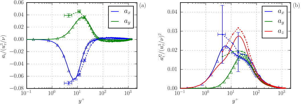 Figure 1
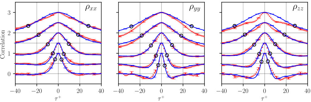 Figure 2
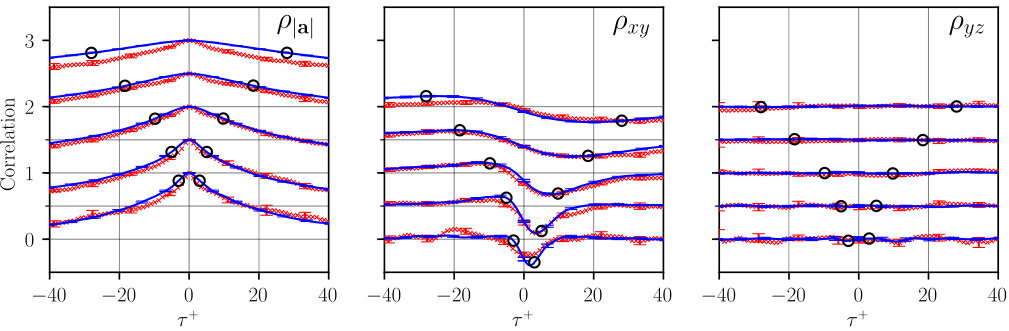 Figure 3
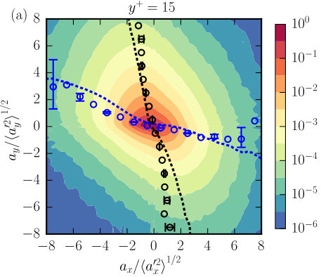 Figure 4
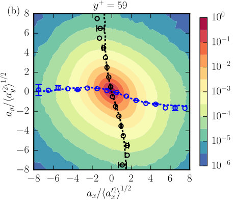 Figure 5
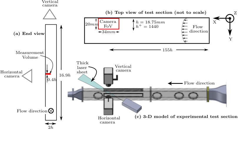 Figure 6
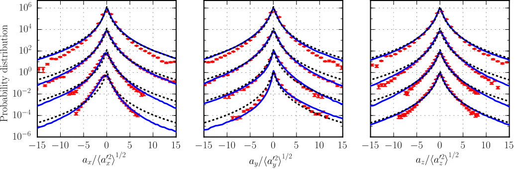 Figure 7
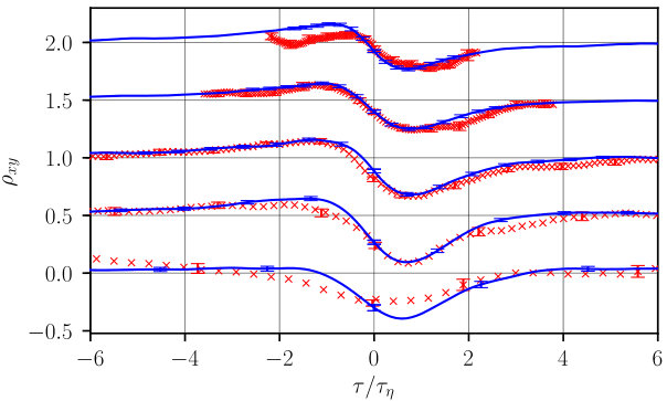 Figure 8
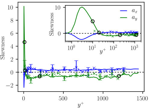 Figure 9
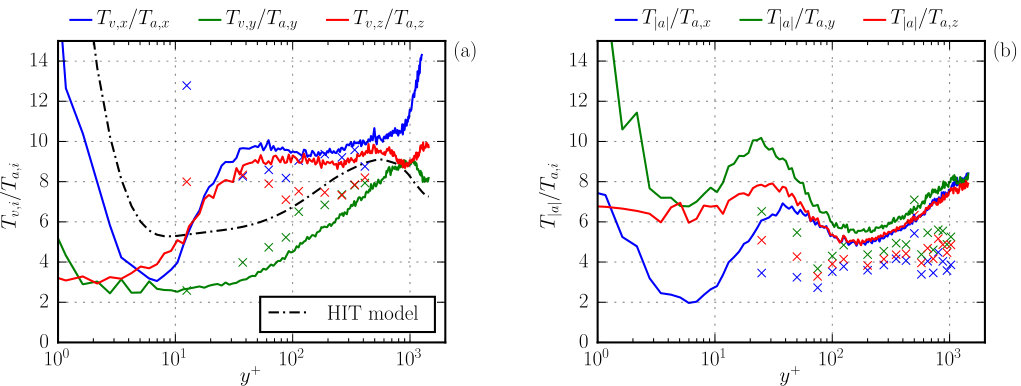 Figure 10
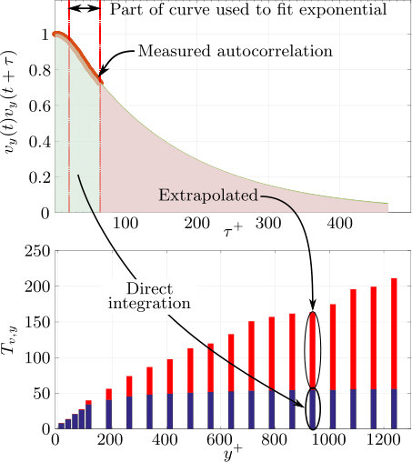 Figure 11
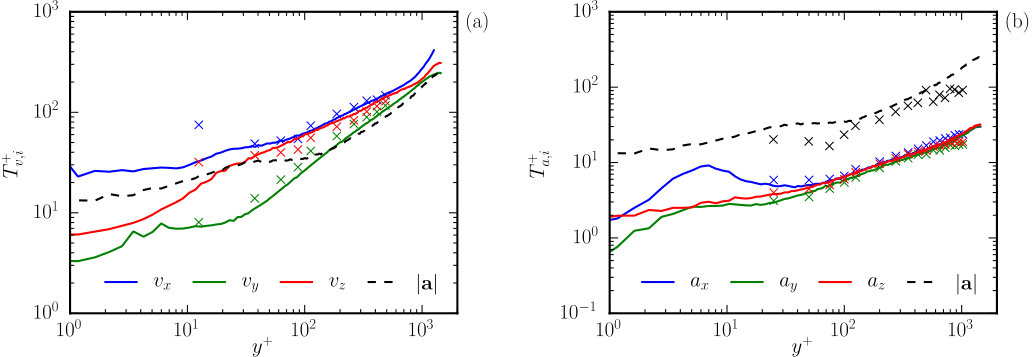 Figure 12
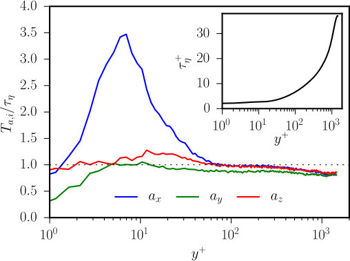 Figure 13
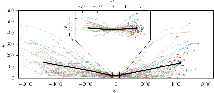 Figure 14
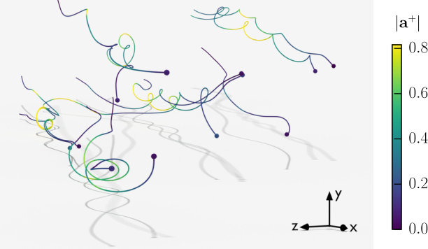 Figure 15
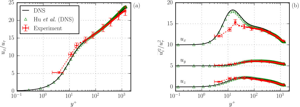 Figure 16
Peer Reviews
No public reviews on file for this paper yet. If you reviewed it on a platform where reviews are public (OpenReview, ICLR, NeurIPS, ICML), you can paste yours below so the community can read it here.
Videos
No videos yet. Explain this paper in a talk, walkthrough, or lecture? Add one.
Lagrangian acceleration statistics in a turbulent channel flow
Nickolas Stelzenmuller
Laboratoire des Ecoulements Géophysiques et Industriels, Université Grenoble Alpes & CNRS, Domaine Universitaire, CS 40700, F-38058 Grenoble, France
Juan Ignacio Polanco
Laboratoire de Mécanique des Fluides et d’Acoustique, UMR 5509, Ecole Centrale de Lyon, CNRS, Université Claude Bernard Lyon 1, INSA Lyon, 36 av. Guy de Collongue, F-69134 Ecully, France
Laure Vignal
Laboratoire des Ecoulements Géophysiques et Industriels, Université Grenoble Alpes & CNRS, Domaine Universitaire, CS 40700, F-38058 Grenoble, France
Ivana Vinkovic
Laboratoire de Mécanique des Fluides et d’Acoustique, UMR 5509, Ecole Centrale de Lyon, CNRS, Université Claude Bernard Lyon 1, INSA Lyon, 36 av. Guy de Collongue, F-69134 Ecully, France
Nicolas Mordant
Laboratoire des Ecoulements Géophysiques et Industriels, Université Grenoble Alpes & CNRS, Domaine Universitaire, CS 40700, F-38058 Grenoble, France
Abstract
Lagrangian acceleration statistics in a fully developed turbulent channel flow at 1440$$ are investigated, based on tracer particle tracking in experiments and direct numerical simulations. The evolution with wall distance of the Lagrangian velocity and acceleration time scales is analyzed. Dependency between acceleration components in the near-wall region is described using cross-correlations and joint probability density functions. The strong streamwise coherent vortices typical of wall-bounded turbulent flows are shown to have a significant impact on the dynamics. This results in a strong anisotropy at small scales in the near-wall region that remains present in most of the channel. Such statistical properties may be used as constraints in building advanced Lagrangian stochastic models to predict the dispersion and mixing of chemical components for combustion or environmental studies.
channel flow; Lagrangian turbulence; acceleration; stochastic models
pacs:
47.27.nd
I Introduction
The Lagrangian study of fluid particle trajectories is a natural first step in predicting the transport of components that are passively entrained by the flow such as chemical/radioactive pollution (passive scalars), aerosols (with small inertia) or the mixing of components prior to combustion. Indeed, in many cases the Péclet number is very large so that most of the statistical properties of scalar dispersion are directly related to that of the dispersion of fluid particles (except of course at the smallest scales at which molecular diffusion plays an ultimate role that depends on the Schmidt number). Despite advances in computational power and resources, direct numerical simulations (DNS) are still out of reach in practical situations. Thus, an efficient modeling is required to obtain reliable predictions. Due to the random nature of turbulence, it is tempting to develop stochastic models that could be used for simulations with an average or large-scale knowledge of the flow. A growingly popular method is Large Eddy Simulation (LES) in which only the largest scales of the turbulence are resolved whereas the small scales of the turbulent spectra are modeled Sagaut (2006). Various classes of models can be used for the unresolved part of the flow, and Lagrangian stochastic subgrid models can be developed for such simulations as used in combustion for instance Pope (1985); Zamansky et al. (2013). An efficient model would also be useful to forecast the dispersion of pollution from localized sources (e.g. industrial accident) using coarse grid meteorological predictions.
In the context of homogeneous and isotropic turbulence (HIT), 1D Lagrangian stochastic models have been developed as variations of the Langevin equation, i.e. modeling the velocity of a fluid particle as a Markovian process Pope (1994):
[TABLE]
with the Lagrangian integral time scale, a Wiener process and the velocity variance. Due to the absence of correlations between velocity components this equation is 1D. It is so strongly constrained by symmetries and the input from the Kolmogorov 1941 theory that it involves only one parameter (with the average turbulent energy dissipation rate per unit mass and a universal constant). This approach incorporates naturally Taylor’s classic result Taylor (1920) of long term turbulent diffusion of a single particle. This equation includes neither the dependency on the Reynolds number nor intermittency. Concerning the former point, this simple framework (equation 1) has been extended by Sawford (1991) to include finite Reynolds number effects. The model is now a second order stochastic equation that models the acceleration and no longer the velocity:
[TABLE]
Parameters and are two inverse time scales related to the Kolmogorov time scale and the integral Lagrangian time scale . The Reynolds number thus appears as the ratio of the two time scales. At very high Reynolds number, the Kolmogorov 1941 theory predicts that the ratio (with the usual Taylor-scale Reynolds number). Sawford Sawford (1991) suggested an empirical formula estimated from DNS at moderate given by:
[TABLE]
This model remains Gaussian at all scales and thus does not include any intermittency effect. Moreover, it remains unidimensional with no interdependency between acceleration (or velocity) components. Real flows as encountered in nature (atmospheric boundary layer) or in industrial applications (pipes, mixers, combustion chambers…) can rarely be considered as homogeneous and isotropic, notably due to non-zero average shear and wall-confinement. Pope (2002) showed that a homogeneous, anisotropic Langevin-type stochastic model should include the time scales associated with the auto- and cross-correlations of the acceleration and velocity components.
The last twenty years have seen the development of experimental techniques and DNS capabilities that have allowed the direct simultaneous observation of the acceleration, velocity, and position of fluid particles, mostly focused on HIT. They showed that acceleration statistics are strongly non-Gaussian (intermittent) La Porta et al. (2001). Modelling such features requires to further increase the dimensionality of the stochastic models in the framework of the non extensive statistical mechanics Pope and Chen (1990); Beck (2001); Reynolds (2003) or to use a non-Markovian model Mordant et al. (2002). In both cases, inspired by the Kolmogorov-Obukhov 1962 theory, dissipation (that appears in the magnitude of the noise in the stochastic equations) is assumed to be itself a stochastic variable and fluctuates with a long time scale comparable to . Thus, the stochastic equations involve multiplicative noise that make their developments much more involved.
Data concerning more realistic flows are scarce Choi et al. (2004); Chen et al. (2010); Walpot et al. (2007); Del Castello and Clercx (2011); Gerashchenko et al. (2008); Tanière et al. (2010); Kuerten and Brouwers (2013). Complex models of inhomogeneous and anisotropic turbulence are weakly constrained by symmetries or scaling considerations and thus require significant experimental or numerical input. Del Castello & Clercx Del Castello and Clercx (2011) studied anisotropic turbulence affected by rotation which remains quite far from realistic flows. Walpot et al. reported some Lagrangian statistics of velocity in the circular pipe flow and their incorporation in stochastic modeling but no acceleration data Walpot et al. (2007). Gerashenko et al. Gerashchenko et al. (2008) studied the case of inertial (heavy) particles in a boundary layer but not the case of the Lagrangian tracers. Chen et al. Chen et al. (2010) provided Eulerian information on the acceleration in a turbulent channel flow but did not discuss the Lagrangian dynamics. Choi et al. Choi et al. (2004) report a numerical analysis of the Lagrangian dynamics of acceleration in a turbulent channel flow but their Reynolds number is relatively low and they discuss neither the coupling between acceleration components nor the time scales. This article reports small scale-resolved Lagrangian experimental measurements in a statistically stationary, high aspect ratio turbulent channel flow, as well as DNS results with parameters matching those of the experiment. Such a flow represents a relatively simple academic framework that incorporates the basic ingredients of real flows: average shear (anisotropy) and confinement (inhomogeneity). In the fully developed part of the flow, the Eulerian statistics of the turbulence are stationary in time and translation-invariant in the streamwise and transverse direction. Thanks to these symmetries, the statistics can be conditioned on a single parameter, the wall distance . This relative simplicity makes this flow a privileged framework to develop and benchmark advanced Lagrangian stochastic models applicable to realistic flows.
It is well known that near-wall turbulence is characterized by multiscale coherent structures with preferential orientations Smits et al. (2011). These structures include intense vortices elongated in the mean flow direction, that strongly affect the near-wall flow dynamics. These streamwise vortices induce strong centripetal accelerations, being the main source of acceleration intermittency near the walls Lee et al. (2004), as illustrated on Fig. 1. On the other hand, large-scale inhomogeneity implies that velocity and acceleration statistics depend on wall distance. Thus, it is also of interest to investigate the far-wall behavior, where a return to isotropy may be expected, and stochastic models based on isotropic turbulence may be applied.
We first present the experimental and numerical setups that allow us to measure the acceleration of particles along their trajectories. In part III we show the statistical analysis of the temporal dynamics through the computation of time correlation functions of both acceleration and velocity components. This analysis provides estimates of the relevant time scales that are discussed in part IV. In part V we focus on the acceleration probability distributions and compare them to the case of HIT.
II Experimental and numerical setups
We study the turbulent flow in a channel between two parallel walls separated by a distance using the same Reynolds number (34,000$$) in both experiments and DNS. This corresponds to a friction Reynolds number , where is the friction velocity associated to the shear stress at the wall and the kinematic viscosity. In the following, the superscript indicates quantities expressed in wall units, nondimensionalized by and .
The experiment consists of measurements made in a closed-loop water tunnel, shown in Fig. 2, with a centerline velocity 1.75\text{,}\mathrm{m}\text{,}{\mathrm{s}}^{-1}$$. We chose water as a working fluid in order to have neutrally buoyant and small enough tracer particles, which is very difficult to achieve in air. The experimental test section is long with a cross-section of , with tripped boundary layers at the entrance. The development length is and the channel height is , ensuring statistical homogeneity in the streamwise and spanwise directions.
The wall unit is 13\text{,}\mathrm{\SIUnitSymbolMicro m}$$ in our experimental conditions, thus we chose to seed the flow with polystyrene spheres that are small enough to accurately trace the flow down to the viscous layer. The Stokes number of these particles ranges from at to at the center of the channel. Fluorescent particles are used in order to improve the contrast in the vicinity of the wall by eliminating reflections of the illumination laser near the wall. This choice makes the measurement conditions quite challenging due to the weak amount of light emitted by the particles. Three dimensional particle trajectories are measured by particle tracking velocimetry Ouellette et al. (2006) in a measurement volume illuminated by a -thick 25W CW laser sheet, using two highly sensitive very high speed Phantom v2511 cameras running at a sampling rate of (with one and one macro lenses with optical filters tuned to the emission frequency of the fluorescent particles). The measurement volume covers half the width of the channel and is long enough in the downstream direction for a sufficiently long time of particle tracking. This allows us to observe the full decorrelation of the acceleration and (close to the wall) the velocity. Such a high sampling rate is required in order to have enough time resolution to differentiate twice the trajectories and compute the acceleration. Particle velocity and acceleration are obtained by convolution of the trajectories with Gaussian differentiating kernels, which also serves to filter out noise from the measurements Mordant et al. (2004a). The pixel size corresponds to in physical space, but thanks to the diffraction of their emitted light, the fluorescent particles cover about three pixels in the images, which has been shown to be a good condition for subpixel position accuracy. Indeed, the estimated accuracy is 1/10th of a pixel (i.e. ) after filtering. Although this allows us to have a fairly precise estimation of the position of the particles in the bulk of the flow, the apparent size of the particle and the existence of images reflected in the wall prevents us from measuring the position of the particles very near the wall. The closest distance at which accurate detection of the particle was possible is , i.e. about . Thus, our range of measurement spans the interval i.e. more than two orders of magnitude in wall distance.
Direct numerical simulations are performed using a pseudo-spectral method for the resolution of the velocity field between two parallel walls, coupled with Lagrangian tracking of passive tracers advected by the resolved fluid velocity. The pseudo-spectral method, described in detail by Buffat et al. (2011), assumes periodicity in the streamwise () and spanwise () directions, where a Fourier decomposition of the velocity field is applied. In the wall-normal () direction, a Chebyshev expansion is performed in order to enforce no-slip boundary conditions at the walls. The size of the computational domain is (in wall units, ) in the streamwise, wall-normal and spanwise directions, respectively. The velocity field is decomposed into spectral modes. In physical space, this corresponds to a uniform grid spacing and in the streamwise and spanwise directions, respectively. In the wall-normal direction, the grid spacing varies between (wall region) and (channel center). An explicit second-order Adams-Bashforth scheme is used to advance the resolved equations in time, with a simulation time step . The total simulation time in channel units is , which corresponds to about turnover times of the centerline flow.
Once the instantaneous velocity field is known, the acceleration field is computed in the Eulerian frame according to . Orzag’s 2/3 rule Orszag (1971) is applied in the and directions to the velocity and acceleration fields to filter out aliasing noise resulting from evaluation of non-linear terms.
The simulation is started with a fully-developed, statistically stationary turbulent channel flow containing randomly distributed fluid particles. Velocity and acceleration of fluid particles are determined from interpolation of the respective Eulerian fields at each particle location using third-order Hermite polynomials. The choice of the interpolation scheme is critical, particularly for the evaluation of Lagrangian acceleration statistics. Lower-order schemes such as trilinear or Lagrange interpolation lead to spurious oscillations which are clearly visible in the temporal spectrum of particle acceleration Choi et al. (2004); van Hinsberg et al. (2013). Particle positions are advanced in time using a second-order Adams-Bashforth scheme, as for the Eulerian velocity field. Sample trajectories obtained from this procedure are shown in Figs. 1 and 5.
In Fig. 3, mean and variance velocity profiles from experiments and simulations are compared with the channel flow DNS of Hu et al. (2006) at roughly the same Reynolds number . Experimental profiles are obtained by sampling the instantaneous velocity of particles conditioned by their wall distance . In the three cases, the mean streamwise velocity profile presents a clear logarithmic behavior over . Results from both simulations are consistent with each other, while slight departures in the mean profile are observed for the experiments. These differences are more pronounced near the wall () and towards the channel center (). Similar remarks can be made for the streamwise velocity variance, where an important difference is found at relative to the simulations. On the other hand, wall-normal and transverse velocity variances from experiments are in agreement with the simulations at all measured wall distances.
Error bars shown on the experimental results in Fig. 3 and the following experimental results reported in this paper (with the exception of the probability density function results discussed in Section V) are calculated statistically for a 95% confidence interval Benedict and Gould (1996). Error bars also take into account the experimental precision associated with the parameters used to report normalized results, , , etc., which is incorporated into the error calculation in the standard way Moffat (1988), and in some cases is responsible for a large part of the error, as in the plot of shown in Fig. 4.
Figure 4 shows the mean and variance acceleration profiles obtained by our experiments and DNS. The profiles are consistent with the DNS results of Yeo et al. (2010) (also presented in the figure) even though their simulations were performed at a considerably lower Reynolds number . As shown by Yeo et al. (2010), the mean streamwise acceleration can be decomposed into an irrotational and a solenoidal contribution, associated with the mean streamwise pressure gradient and the viscous stress, respectively. In wall units, this is expressed as . Near the wall, the solenoidal term dominates and is negative, which shows that the negative peak of mean streamwise acceleration at is a consequence of a viscous contribution. For the mean wall-normal acceleration, the solenoidal term is zero. Therefore, its profile is entirely determined by the mean wall-normal pressure gradient Yeo et al. (2010).
Profiles of acceleration variance (Fig. 4b) reveal qualitative agreement between both sets of data, although large uncertainty is seen in the experimental results near the wall. It is worth noting that, at their respective peaks, the standard deviation of acceleration is larger than the magnitude of the mean acceleration, indicating that dynamics near the wall are strongly influenced by acceleration fluctuations. As shown by Lee et al. (2004), these dynamics are dominated by the presence of near-wall streamwise vortices inducing high-magnitude, oscillating centripetal accelerations mainly oriented in the spanwise and wall-normal directions.
III Lagrangian correlations
The Lagrangian description deals with particle trajectories that are parameterized by their initial position and by the time delay relative to the initial time . In stationary HIT, Lagrangian statistics do not depend on due to translational invariance, nor on due to statistical stationarity. Statistics are thus parametrized only by the time delay . Furthermore, single-point single-time statistics such as moments of acceleration components are constant in . In inhomogeneous turbulence, things are more complex. Indeed the initial position must be retained. The symmetries of the channel flow are such that the dependency of the statistics on reduces to a dependency on the initial distance from the wall, . Moreover, single-time Lagrangian statistics now vary with the time delay . For instance, the Lagrangian average of the streamwise velocity component, , depends on because particles move away from their initial distance (toward the center on average, see Fig. 5) and thus experience regions of higher average velocity.
In inhomogeneous flows, the Lagrangian and Eulerian averages coincide only for . Stationarity of Eulerian statistics implies that Lagrangian statistics depend only on and and not on . Inhomogeneity also implies that Lagrangian statistics for negative values of are a priori different from those at positive . Practically, estimators of Lagrangian statistics are the following. A small interval of width around a given initial value of is chosen. As soon as a trajectory has a value that belongs to this interval, the initial time is set. Statistics are then accumulated as a function of . This procedure is illustrated in Fig. 5 for the average particle position .
An adequate tool to obtain time scales and coupling between components is the Lagrangian correlation coefficient of fluid particle acceleration, defined as
[TABLE]
where is the fluid particle acceleration fluctuation relative to the Lagrangian average, with or . The estimators thus correlate the initial acceleration with that at a time lag along the trajectory of fluid particles initially at .
Figures 6 and 7 show various components of the acceleration correlation tensor calculated at different initial wall distances . Time lags equal to the local Kolmogorov time scale are also represented in the figures, with the local mean turbulent energy dissipation rate estimated from DNS as .
The inhomogeneity of the flow is visible in the fact that the typical decorrelation time varies significantly over the width of the channel. The anisotropy is visible in the fact that the streamwise and wall-normal components display some non zero correlation (in contrast with HIT), as shown on Fig 7(b). Cross-correlations with the transverse component remain zero due to the statistical symmetry , as shown on Fig. 7(c).
In the vicinity of the wall the decorrelation time is close to one in wall units, showing that this is the adequate characteristic time for rescaling of small-scale quantities such as the acceleration in this region. This will be discussed further in the analysis of the characteristic Lagrangian time scales. A very good agreement is observed between experimental and DNS results, with the exception of the long time behavior of at , and the short time behavior of at . While the former remains unexplained, the latter is due to the higher level of noise in the measurement of the -component, which is a technical consequence of the way the PTV is performed. Namely, near the center of the channel, the signal-to-noise ratio for the -component of acceleration comes close to the limits of the data processing methods described in Section II and in previous work Mordant et al. (2004a), and the correlation of noise is seen in the short time behavior of at .
Previous studies in HIT Mordant et al. (2004b); Toschi et al. (2005) have associated fluid particle acceleration and vortex dynamics by observing that high acceleration events often correspond to centripetal accelerations in vortex filaments, and the auto-correlation of the centripetal component of these accelerations become negative to a much greater degree than the auto-correlation of the component of the acceleration parallel to the vortex filament. Contrary to HIT where there are no preferential directions, in the near-wall region of a wall-bounded turbulent flow the preferential orientation of vortices in the streamwise direction is expected. As shown on Fig. 6, near the wall the auto-correlations of and become negative at approximately (similarly to the case of HIT), while the correlation of remains positive with a significantly longer initial decorrelation time. The negative and correlations can be associated with the effect of near-wall streamwise vortices. A fluid particle trapped in one such vortex experiences strong centripetal accelerations towards the vortex rotation axis Lee et al. (2004). This strong form of anisotropy of the acceleration is only observed near the walls () and becomes negligible towards the channel center, as confirmed below by the acceleration time scales associated to these correlations.
The auto-correlations and are almost symmetric in time, e.g. . This symmetry can be explained by the nearly time-symmetric average trajectories in the near-wall region as illustrated in Fig. 5, i.e. . In contrast, the cross-correlation is strongly time-asymmetric close to the wall. This asymmetry, along with the non-zero time lag at which the peak is observed, suggests the idea of causality between acceleration components. That is, a streamwise acceleration fluctuation is followed on average by an opposite-sign wall-normal acceleration fluctuation. Towards the channel center, this effect persists and the correlation becomes antisymmetric with time, , due to the decreasing influence of wall confinement.
The correlation between and (Fig. 7(b)) is most important near the walls. In that region, the zero-time cross-correlation (equivalent to an Eulerian single-point single-time correlation) is negative due to increased viscous effects combined with confinement by the wall (see the joint PDFs in Section V for more details). Moreover, the cross-correlation peak is always found at a non-zero time lag. Far from the wall, the correlation is close to zero at , while it increases in absolute value for non-zero time lags. The influence of the boundary layer remains visible even in the bulk of the channel where the correlation is still non-zero, indicating that small-scale anisotropy is still present in that region. In Fig. 8, the cross-correlation is displayed as function of the normalized time lag . The time lag of the negative correlation peak is shown to scale with , with a value fluctuating between and with the wall distance .
The correlation describes the changes of orientation of the acceleration fluctuation vector projected on the - plane. Its behavior implies that there is a preferential direction of rotation of along a particle trajectory. Moreover, such changes of orientation happen over times of the order of the Kolmogorov time scale. Thus, this anisotropy is associated with the smallest scales of turbulence, and is observed for all wall distances. The preferential direction of rotation implied by the cross-correlation is consistent with the direction of mean shear, represented by an average vorticity which is negative in the lower half of the channel, where the presented statistics are obtained. This result is consistent with evidence of small-scale anisotropy found in other turbulent flows governed by large-scale anisotropy. For instance, from DNS of homogeneous shear flow, Pumir and Shraiman (1995) found signs of small-scale anisotropy which did not decrease at increasing Reynolds number, in contradiction with Kolmogorov’s local isotropy hypothesis Kolmogorov (1941). In their work, small-scale anisotropy was quantified by the skewness of the spanwise vorticity , which was shown to be of the same sign as the large-scale average vorticity. More recently, and using a similar approach, Pumir et al. (2016) showed the presence of small-scale anisotropy from DNS of turbulent channel flow at all along the log-layer. Our results show that such small-scale anisotropy is also observed by the Lagrangian acceleration statistics. Therefore, a stochastic model for the Lagrangian acceleration which includes elements derived from the correlation would be able to reproduce the presence of small-scale anisotropy in shear flows.
In Fig. 7(a) we plot the auto-correlation of the acceleration magnitude , showing that this quantity stays correlated for far longer than each acceleration component. This behavior is observed at all wall distances and is consistent with results in HIT Yeung and Pope (1989); Mordant et al. (2004c). It is explained by the fact that changes in the orientation of the acceleration vector are much more sudden than changes in its magnitude. In near-wall turbulence, this observation is again explained by centripetal acceleration induced by streamwise vortices, which preserve the acceleration magnitude for a longer time than the acceleration orientation Lee et al. (2004).
IV Lagrangian time scales
The characteristic time scale associated to each acceleration component is estimated according to
[TABLE]
where is the time lag at which the auto-correlation first crosses . This definition is chosen because the classical definition with the integration going to infinite time cannot be applied to all acceleration components since some correlations become negative. This is also the case for HIT for which the integral of the acceleration correlations is actually zero because of the stationarity of the velocity. The usual zero-crossing time as in Yeung and Pope (1989) can neither be used here because some correlations (near the center of the channel) do not cross zero during the observation time. Our definition is a convenient mix between these two usual definitions of the typical time scale.
Lagrangian velocity (integral) time scales , as well as the acceleration norm time scale , are defined equivalently. Due to the limited measurement volume in the experiment, the full decorrelation of the auto-correlations of velocity and the norm of the acceleration is not achieved at all wall distances in the channel. These auto-correlations have been extrapolated as illustrated by Fig. 9, and the uncertainty of these results increases with increased extrapolation. This extrapolation is not necessary for the acceleration auto-correlations shown in Fig. 6 (which decay much faster) and thus for the computation of the time scales .
The evolution of all time scales with wall distance is shown in Fig. 10. As can be deduced from the auto-correlation curves, the acceleration time scales and generally increase with wall distance. The same is observed for the Lagrangian velocity time scales. The acceleration norm time scale is about one order of magnitude larger than the time scale of the acceleration components. It is of the order of the integral time scales .
In Fig. 11, the Lagrangian acceleration time scales are normalized with the local Kolmogorov time scale. Both and vary with wall distance. The acceleration time scales are of the order of all along the channel. The normalized time scales only weakly change for , reaching a value between 0.8 and 0.9 in the bulk of the channel. However, in that region, small differences persist between and the time scales obtained for the other two components, suggesting once more that anisotropy is still present far from the wall. Close to the wall (), the longer correlation time of the streamwise acceleration is reflected in a larger time scale compared to the other components.
Fig. 12(a) shows the ratio of Lagrangian time scales of velocity and acceleration for each component. Also shown in Fig. 12(a) is eq. (3), the empirical fit to the DNS data of Yeung and Pope Yeung and Pope (1989) proposed by Sawford Sawford (1991), using the profile of calculated from the DNS and as suggested by Sawford. The HIT model follows the trend of the data. However there is significant anisotropy in these ratio of time scales that extends far away from the wall. First-order Lagrangian stochastic models in velocity such as given by eq. (1) are based implicitly on the scale separation between the velocity and the acceleration time scales. Here, a small separation is seen between these two time scales near the wall. Significantly, the time scale ratio for the wall-normal component () is approximately half of that predicted by the local Reynolds number (the HIT model plotted in the figure) near the wall. Even farther from the wall, this time scale ratio is significantly over-predicted by the HIT model.
The long time scales of the acceleration norm previously reported have inspired the development of a Lagrangian subgrid stochastic model that models the acceleration norm and acceleration direction as two independent stochastic processes Sabel’nikov et al. (2011); Zamansky et al. (2013). Fig. 12(b) shows that the ratio of Lagrangian time scales of acceleration norm to acceleration components are only weakly varying for and comparable in magnitude to the ratios of Lagrangian velocity and acceleration time scales.
V Distributions
Fig. 13 shows the probability distribution function (PDF) of the three acceleration components obtained at different wall distances. All curves present very long tails corresponding to extremely high acceleration events associated to intermittency La Porta et al. (2001). Once again, good agreement is achieved between the experiments and the DNS. The acceleration PDFs are also compared with the functional shape proposed by Mordant et al. (2004c) for HIT, which assumes that the acceleration magnitude follows a log-normal probability distribution and that the acceleration vector is isotropic. According to those assumptions, the PDF of an acceleration component is given by
[TABLE]
where determines the variance of ( for variance 1), while determines the shape of the PDF. A value is used in the comparisons. Towards the channel center, the PDFs of the three acceleration components match this prediction, suggesting that the instantaneous behavior of acceleration becomes close to isotropic. More strikingly, the spanwise acceleration seems to match the prediction very close to the wall, suggesting that this component is not affected by anisotropy as in the other two directions. The general agreement with the shape of the HIT PDF suggests that intermittency is extremely strong in the boundary layer although the Reynolds number is moderate: to in our flow whereas it was close to 1000 in Mordant et al. (2004c). It implies also that this shape of the PDF presents some universality.
The PDFs of the streamwise and wall-normal acceleration components become quite asymmetric near the wall. This asymmetry is quantified by their skewness shown in Fig. 14. Due to flow symmetry, the skewness of is zero. Very close to the wall, and are strongly negative and positive, respectively, indicating that their PDFs are very asymmetric due to wall-induced anisotropy. The signs of and are both inverted after . Their respective values remain different from zero and change little for . This reinforces the idea that turbulence anisotropy is still present in the channel center.
The dependency between the acceleration components is analyzed by the joint PDF, . Fig. 15 shows the results obtained at two wall distances, and . Close to the wall (Fig. 15a), the joint PDF has a stretched shape, showing a preference for events given by and . These events can be associated to fluid particles advected towards the wall. These particles move towards regions of decreasing mean streamwise velocity, leading on average to a streamwise deceleration of their motion (). Simultaneously, their negative wall-normal velocity goes to zero due to confinement by the wall, resulting in a positive wall-normal acceleration (). This dependency between both acceleration components is confirmed by the conditional means and , which are superposed to the joint PDF contours. Particles advected away from the wall are less affected by wall confinement, and thus the impact on their wall-normal acceleration is less visible in the joint PDF. Nonetheless, on average, those particles also experience the effect of the mean velocity gradient, which results in this case in a positive streamwise acceleration.
VI Concluding remarks
By performing both DNS and experiments, the highly anisotropic turbulent flow in the vicinity of channel walls is described in terms of Lagrangian statistics. Near-wall vortical structures are clearly identified by their influence on the acceleration auto-correlations. Viscous effects and wall-confinement have also a strong impact on acceleration statistics as evidenced by the joint PDFs. Less expectedly, signs of small-scale anisotropy are present across the channel. The observed behavior of the Lagrangian time scales can be a basis for the formulation of Lagrangian stochastic models of acceleration applied to wall-bounded turbulent flows. These models must also take into account the dependency among acceleration components, which is apparent in the presented cross-correlations and joint PDFs of acceleration. Acceleration models based on the presented results should be able to capture the effects of (i) the near-wall dynamics associated with confinement and coherent structures and (ii) the small-scale anisotropy present in the whole channel.
Acknowledgements.
This work is supported by Agence Nationale de la Recherche (grant #ANR-13-BS09-0009) and by the LabEx Tec 21 (Investissements d’Avenir grant #ANR-11-LABX-0030). Simulations have been performed on the P2CHPD cluster. J.I.P. is grateful to CONICYT Becas Chile grant No. 72160511 for supporting his work. NM is supported by Institut Universitaire de France. We thank Laboratoire de Physique at ENS de Lyon and CNRS for providing one of the high speed cameras. We thank M. Kusulja for the design of the water tunnel, J. Virone and V. Govart for technical assistance.
The reference list from the paper itself. Each links out to its DOI / PubMed record.
- 1Sagaut (2006) P. Sagaut, Large Eddy Simulation for Incompressible Flows: An Introduction , 3rd ed. (Springer, Berlin, New York, 2006).
- 2Pope (1985) S. B. Pope, “PDF methods for turbulent reactive flows,” Prog. Energy Combust. Sci. 11 (1985).
- 3Zamansky et al. (2013) R. Zamansky, I. Vinkovic, and M. Gorokhovski, “Acceleration in turbulent channel flow: universalities in statistics, subgrid stochastic models and an application,” J. Fluid Mech. 721 , 627–668 (2013) . · doi ↗
- 4Pope (1994) S. B. Pope, “Lagrangian PDF methods for turbulent flows,” Ann. Rev. Fluid Mech. 26 (1994).
- 5Taylor (1920) G. I. Taylor, “Diffusion by continuous movements,” Proc Lond. Math Soc 20 , 196–212 (1920) .
- 6Sawford (1991) B. L. Sawford, “Reynolds number effects in Lagrangian stochastic models of turbulent dispersion,” Phys. Fluids A 3 , 1577–1586 (1991) . · doi ↗
- 7Pope (2002) S. B. Pope, “Stochastic Lagrangian models of velocity in homogeneous turbulent shear flow,” Phys. Fluids 14 , 1696–1702 (2002) . · doi ↗
- 8La Porta et al. (2001) A. La Porta, Greg A. Voth, Alice M. Crawford, J. Alexander, and E. Bodenschatz, “Fluid particle accelerations in fully developed turbulence,” Nature 409 , 1017–1019 (2001) . · doi ↗