Nonlinear approximation with nonstationary Gabor frames
Emil Solsb{\ae}k Ottosen, Morten Nielsen

TL;DR
This paper investigates the sparseness of adaptive time-frequency representations using nonstationary Gabor frames, characterizing signals with sparse expansions and providing bounds on approximation errors, supported by numerical experiments.
Contribution
It establishes a theoretical link between sparseness and smoothness in nonstationary Gabor expansions and offers practical bounds on approximation errors.
Findings
Sparse expansions correspond to smooth signals in a specific decomposition space.
An upper bound on approximation error from thresholding coefficients is proven.
Numerical experiments confirm the theoretical approximation rates.
Abstract
We consider sparseness properties of adaptive time-frequency representations obtained using nonstationary Gabor frames (NSGFs). NSGFs generalize classical Gabor frames by allowing for adaptivity in either time or frequency. It is known that the concept of painless nonorthogonal expansions generalizes to the nonstationary case, providing perfect reconstruction and an FFT based implementation for compactly supported window functions sampled at a certain density. It is also known that for some signal classes, NSGFs with flexible time resolution tend to provide sparser expansions than can be obtained with classical Gabor frames. In this article we show, for the continuous case, that sparseness of a nonstationary Gabor expansion is equivalent to smoothness in an associated decomposition space. In this way we characterize signals with sparse expansions relative to NSGFs with flexible time…
Click any figure to enlarge with its caption.
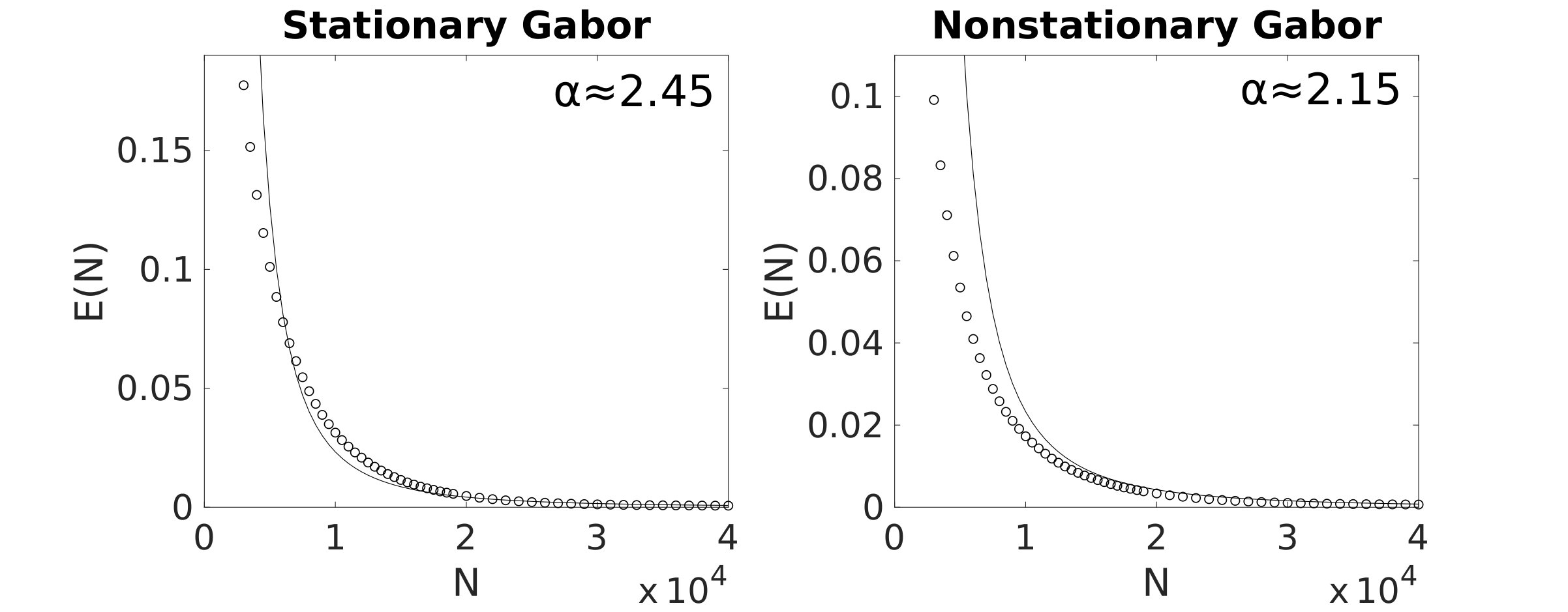 Figure 1
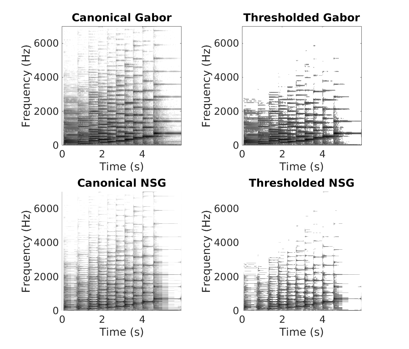 Figure 2
| Transform: | G | G | G | NSGF |
|---|---|---|---|---|
| Average redun.: | ||||
| Average error: | ||||
| Average : |
Peer Reviews
No public reviews on file for this paper yet. If you reviewed it on a platform where reviews are public (OpenReview, ICLR, NeurIPS, ICML), you can paste yours below so the community can read it here.
Videos
No videos yet. Explain this paper in a talk, walkthrough, or lecture? Add one.
Nonlinear approximation with nonstationary Gabor frames
Emil Solsbæk Ottosen
and
Morten Nielsen
Department of Mathematical Sciences, Aalborg University, Skjernvej 4, 9220 Aalborg Ø, Denmark
Abstract.
We consider sparseness properties of adaptive time-frequency representations obtained using nonstationary Gabor frames (NSGFs). NSGFs generalize classical Gabor frames by allowing for adaptivity in either time or frequency. It is known that the concept of painless nonorthogonal expansions generalizes to the nonstationary case, providing perfect reconstruction and an FFT based implementation for compactly supported window functions sampled at a certain density. It is also known that for some signal classes, NSGFs with flexible time resolution tend to provide sparser expansions than can be obtained with classical Gabor frames. In this article we show, for the continuous case, that sparseness of a nonstationary Gabor expansion is equivalent to smoothness in an associated decomposition space. In this way we characterize signals with sparse expansions relative to NSGFs with flexible time resolution. Based on this characterization we prove an upper bound on the approximation error occurring when thresholding the coefficients of the corresponding frame expansions. We complement the theoretical results with numerical experiments, estimating the rate of approximation obtained from thresholding the coefficients of both stationary and nonstationary Gabor expansions.
Key words and phrases:
Time-frequency analysis, nonstationary Gabor frames, sparse frame expansions, decomposition spaces, nonlinear approximation
2010 Mathematics Subject Classification:
41A17, 42B35, 42C15, 42C40
1. Introduction
The field of Gabor theory [19, 6, 41] is concerned with representing signals as atomic decompositions using time-frequency localized atoms. The atoms are constructed as time-frequency shifts of a fixed window function, according to some lattice parameters, such that the resulting system constitutes a frame and, therefore, guarantees stable expansions [5, 35, 31]. Such frames are known under the name of Weyl-Heisenberg frames or Gabor frames and have been proven useful in a variety of applications [22, 10, 33]. The structure of Gabor frames implies a time-frequency resolution which depends only on the lattice parameters and the window function. In particular, the resolution is independent of the signal under consideration, which makes the corresponding implementation fast and easy to handle. The usage of a predetermined time-frequency resolution naturally raises the question of whether an improvement can be obtained by taking the signal class into consideration? This question has lead to many interesting approaches for constructing adaptive time-frequency representations [11, 27, 40, 42]. Unfortunately, for representations with resolution varying in both time and frequency there seems to be a trade-off between perfect reconstruction and fast implementation [30]. In this article, we therefore consider time-frequency representations with resolution varying in either time or frequency. The idea is to generalise the theory of painless nonorthogonal expansions [6] to the situation where multiple window functions are used along either the time- or the frequency axis. The resulting systems, which allow for perfect reconstruction and an FFT based implementation, are called painless generalised shift-invariant systems [36, 25] or painless nonstationary Gabor frames (painless NSGFs) [26, 1]. As already noted in [1], painless NSGFs tend to produce sparser representations than classical Gabor frames for certain classes of music signals. Sparseness of a time-frequency representation is desirable for several reasons, mainly because it may reduce the computational cost for manipulating and storing the coefficients [18, 8]. Additionally, many signal classes are characterized by some kind of sparseness in time or frequency and the corresponding signals are, therefore, best described by a sparse time-frequency representation. For such signals, the task of feature identification also benefits from a sparse representation as the particular characteristics of the signal becomes easier to identify.
In this article we consider sparseness properties of painless NSGFs with resolution varying in time. Whereas modulation spaces [14, 22, 16] have turned out to be the proper function spaces for analyzing sparseness properties of classical Gabor frames [23], we need a more general framework for the nonstationary case. A painless NSGF with flexible time resolution corresponds to a sampling grid which is irregular over time but regular over frequency for each fixed time point. We therefore search for a smoothness space which is compatible with a (more or less) arbitrary partition of the time domain. Such a flexibility can be provided by decomposition spaces, as introduced by Feichtinger and Gröbner in [17, 15]. Decomposition spaces may be viewed as a generalization of the classical Wiener amalgam spaces [13, 24] but with no assumption of an upper bound on the measure of the members of the partition. Another way of stating this is that decomposition spaces are constructed using bounded admissible partitions of unity [17] instead of bounded uniform partitions of unity [13]. The partitions we consider are obtained by applying a set of invertible affine transformations on a fixed set [2].
We use decomposition spaces to characterize signals with sparse expansions relative to painless NSGFs with flexible time resolution. We measure sparseness of an expansion by a mixed norm on the coefficients and show that the sparseness property implies an upper bound on the approximation error obtained by thresholding the expansion. Using the terminology from nonlinear approximation, such an upper bound is also known as a Jackson inequality [8, 4]. A similar characterization for classical Gabor frames using modulation spaces was proven by Gröchenig and Samarah in [23]. For the nonstationary case, we provided a characterization in [32] for painless NSGFs with flexible frequency resolution using decomposition spaces. A different approach to this problem is considered by Voigtlaender in [39], where the painless assumption is replaced with a more general analysis of the sampling parameter. The decomposition spaces considered in both [32] and [39] are based on partitions of the frequency domain, which is not a natural choice for NSGFs with flexible time resolution. In this article we consider decompositions of the time domain, which allow for compactly supported window functions sampled at a low density (compared to the general theory formulated in [39]). It is worth noting that there is a significant mathematical difference between decomposition spaces in time and in frequency.
The structure of this this article is as follows. In Section 2 we formally introduce decomposition spaces in time and prove several important properties of these spaces. Then, based on the ideas in [32], we show in Section 3 how to construct a suitable decomposition space for a given painless NSGF with flexible time resolution. In Section 4 we prove that the suitable decomposition space characterizes signals with sparse frame expansions and we provide an upper bound on the approximation rate occurring when thresholding the frame coefficients. Finally, in Section 5 we present the numerical results and in Section 6 we give the conclusions.
Let us now briefly go through our notation. By we denote the Fourier transform with the usual extension to . With we mean that there exist two constants such that . For two normed vector spaces and , means that and for some constant and all . We say that a non-empty open set is compactly contained in an open set if and is compact. We call a separated set if . Finally, by we denote the identity operator on and by we denote the indicator function for a set .
2. Decomposition spaces
In this section we define decomposition spaces [17] based on structured coverings [2]. For an invertible matrix , and a constant , we define the affine transformation with . Given a family of invertible affine transformations on , and a subset , we let and
[TABLE]
We say that is an admissible covering of if and there exists such that for all .
Definition 2.1** (moderate weight).**
Let be an admissible covering. A function is called moderate if there exists such that for all and all . A moderate weight (derived from ) is a sequence with for all .
For the rest of this article, we shall use the explicit choice for the function in Definition 2.1. Let us now define structured coverings [2] of the time domain.
Definition 2.2** (Structured covering).**
Given a family of invertible affine transformations on , suppose there exist two bounded open sets , with compactly contained in , such that
- (1)
and are admissible coverings. 2. (2)
There exists a separated set , with for all , such that is a moderate weight.
Then we call a structured covering.
For a structured covering we have the associated concept of a bounded admissible partition of unity (BAPU) [17].
Definition 2.3** (BAPU).**
Let be a structured covering of . A BAPU subordinate to is a family of non-negative functions satisfying
- (1)
. 2. (2)
.
We note that the assumptions in Definition 2.3 implies that the members of the BAPU are uniformly bounded, i.e., .
Given a structured covering , we can always construct a subordinate BAPU. Choose a non-negative function , with for all and , and define
[TABLE]
for all . With this construction, it is clear that Definition 2.3(1) is satisfied. Further, since is an admissible covering, then for all which shows that Definition 2.3(2) holds.
Remark 2.1**.**
We note that the assumption in Definition 2.2(2) is not necessary for constructing a subordinate BAPU, however, the assumption is needed for proving Theorem 2.1.
Let be a structured covering with moderate weight and BAPU . For and , we define the associated weighted sequence space
[TABLE]
Given , we define by . Since is moderate, defines a bounded operator on according to [17, Remark 2.13 and Lemma 3.2]. Denoting its operator norm by , we have
[TABLE]
We now define decomposition spaces as first introduced in [17].
Definition 2.4** (Decomposition space).**
Let be a structured covering with moderate weight and BAPU . For and , we define the decomposition space as the set of distributions satisfying
[TABLE]
Remark 2.2**.**
According to [17, Theorem 3.7], is independent of the particular choice of BAPU and different choices yield equivalent norms. Actually the results in [17] show that is invariant under certain geometric modifications of , but we will not go into detail here.
Remark 2.3**.**
In contrast to the approach taken in [32] (where the decomposition is performed on the frequency side), we do not allow in Definition 2.4 since a simple consideration shows that the resulting decomposition spaces would not be complete in this case.
We now consider some familiar examples of decomposition spaces. By standard arguments it is easy to verify that with equivalent norms for any structured covering . The next example shows how to construct Wiener amalgam spaces.
Example 2.1**.**
Let be an open cube with center [math] and side-length . Define , with for all , and let . With , then corresponds to the Wiener amalgam space for and , see [13] for further details. ∎
Let us now prove the following important properties of decomposition spaces.
Theorem 2.1**.**
Let be a structured covering with moderate weight and subordinate BAPU . For and ,
- (1)
. 2. (2)
* is a Banach space.* 3. (3)
If , then is dense in . 4. (4)
If , then the dual space of can be identified with with and .
The proof of Theorem 2.1 can be found in Appendix A. In the next section we construct decomposition spaces, which are compatible with the structure of painless NSGFs with flexible time resolution.
3. Nonstationary Gabor frames
In this section, we construct NSGFs with flexible time resolution using the notation of [1]. Given a set of window functions , with corresponding frequency sampling steps , then for we define atoms of the form
[TABLE]
The choice of as index set for is only a matter of notational convenience; any countable index set would do.
Example 3.1**.**
With and for all we get
[TABLE]
which just corresponds to a standard Gabor system. ∎
If for all , we refer to as an NSGF. For an NSGF , the frame operator
[TABLE]
is invertible and we have the expansions
[TABLE]
with being the canonical dual frame of [5]. For notational convenience we define . With this notation we have the following result [1, Theorem 1].
Theorem 3.1**.**
Let with frequency sampling steps , for all . Assuming supp, with for all , the frame operator for the system
[TABLE]
is given by
[TABLE]
The system constitutes a frame for , with frame-bounds , if and only if
[TABLE]
and the canonical dual frame is then given by
[TABLE]
Remark 3.1**.**
We note that the canonical dual frame in (3.2) posses the same structure as the original frame, which is a property not shared by general NSGFs. We also note that the canonical tight frame can be obtained by taking the square root of the denominator in (3.2).
Traditionally, an NSGF satisfying the assumptions of Theorem 3.1 is called a painless NSGF, referring to the fact that the frame operator is a simple multiplication operator. This terminology is adopted from the classical painless nonorthogonal expansions [6], which corresponds to the painless case for classical Gabor frames. By slight abuse of notation we use the term ”painless” to denote the NSGFs satisfying Definition 3.1 below. In order to properly formulate this definition, we first need some preliminary notation which we adopt from [32].
Let satisfy the assumptions in Theorem 3.1. Given we denote by the open cubes
[TABLE]
with for all . We note that supp for all . For we define
[TABLE]
using the notation of (2.1).
Definition 3.1** (Painless NSGF).**
Let satisfy the assumptions in Theorem 3.1, and assume further that,
- (1)
There exists and , such that the open cubes , given in (3.3), satisfy uniformly for all . 2. (2)
is a separated set and constitutes a moderate weight. 3. (3)
The ’s are continuous, real valued and satisfy
[TABLE]
for some uniform constant .
Then we refer to as a painless NSGF.
The assumptions in Definition 3.1 are easily satisfied, but the support condition in Theorem 3.1 is rather restrictive and implies a certain redundancy of the system. Nevertheless, we must assume some structure on the dual frame, which is not provided by general NSGFs. We choose the framework of painless NSGFs and base our arguments on the fact that the dual frame possess the same structure as the original frame. We expect it is possible to extend the theory developed in this article to a more general settings by imposing general existence results for NSGFs [26, 12, 39]. We now provide a simple example of a set of window functions satisfying Definition 3.1(3).
Example 3.2**.**
Choose a continuous real valued function with supp. For define
[TABLE]
with and . Then supp and Definition 3.1(3) is satisfied. ∎
Following the approach taken in [32], we define together with the set of affine transformations with
[TABLE]
It is then easily shown that forms a structured covering of [32, Lemma 4.1]. Given and , we may therefore construct the associated decomposition space with .
Example 3.3**.**
Let be a painless NSGF according to Definition 3.1. Assume additionally that and that Definition 3.1(1) and Definition 3.1(2) hold for the larger cubes for some . Defining and , with
[TABLE]
we obtain the structured covering . In this special case the associated decomposition space is the Wiener amalgam space for and (cf. Example 2.1). ∎
For the rest of this article, we write for a painless NSGF with associated structured covering . With this notation, then supp for all and all . Similarly we write for the associated weight function.
4. Characterization of decomposition spaces
Using the notation of [2] we define the sequence space as the set of coefficients satisfying
[TABLE]
for and . We can now prove the following important stability result.
Theorem 4.1**.**
Let be a painless NSGF with associated structured covering and weight function . Fix , and let . For and ,
[TABLE]
and for and ,
[TABLE]
Proof.
We first prove (4.1). Given , since on , then
[TABLE]
with being the frequency sampling step. Since we can use the Hausdorff-Young inequality [28, Theorem 2.1 on page 98], which together with Definition 3.1(3) imply
[TABLE]
Hence, using (2.2) we get
[TABLE]
Let us now prove (4.2). Given we may write the norm as
[TABLE]
since the dual space of can be identified with and since is dense in . Given , with , we write the frame expansion of with respect to and apply Hölder’s inequality twice to obtain
[TABLE]
According to (4.1) then
[TABLE]
which combined with (4) and (3.1) yield
[TABLE]
with . Finally, combining (4.3) and (4) we arrive at
[TABLE]
which proves (4.2). ∎
We note that for , and , Theorem 4.1 yields the equivalence
[TABLE]
It follows that the coefficient operator is bounded from into . We define the corresponding reconstruction operator as
[TABLE]
With this notation we have the following result.
Proposition 4.1**.**
Let be a painless NSGF with associated structured covering and weight function . Given and , the reconstruction operator is bounded from onto and we have the expansions
[TABLE]
with unconditional convergence.
Proof.
We first prove that is bounded. Given , (2.2) and (3.1) yield
[TABLE]
Applying Definition 3.1(3) and the Hausdorff-Young inequality [28, Theorem 2.2 on page 99] we get
[TABLE]
Combining (4) and (4.8) we arrive at
[TABLE]
which shows the boundedness of . Let us now prove the unconditional convergence of (4.6). Given we can find a sequence such that in . For each we have the expansion and by continuity of we get . Given , (4) implies that we can find a finite subset , such that for all finite sets ,
[TABLE]
According to [22, Proposition 5.3.1 on page 98], this property is equivalent to unconditional convergence. ∎
Based on Proposition 4.1, we can show some important properties of in connection with nonlinear approximation theory [8, 7]. Assume , for , and write the frame expansion
[TABLE]
Let be a rearrangement of the frame coefficients such that constitutes a non-increasing sequence. Also, let be the -term approximation to obtained by extracting the terms in (4.10) corresponding to the largest coefficients . Since is bounded, [20, Theorem 6] implies that for each ,
[TABLE]
We conclude that for , with frame coefficients in , we obtain good approximations in by thresholding the frame coefficients in (4.10). The rate of the approximation is given by .
5. Numerical experiments
In this section we provide the numerical experiments, thresholding coefficients of both stationary and nonstationary Gabor expansions. We note that analyzis with a stationary Gabor frame corresponds to analyzis with the short-time Fourier transform (STFT) as the Gabor coefficients can be re-written as
[TABLE]
with denoting the STFT of , with respect to , at time and frequency .
For the implementation we use MATLAB 2017B and in particular we use the following two toolboxes: The LTFAT [34] (version 2.2.0 or above) available from http://ltfat.github.io/ and the NSGToolbox [1] (version 0.1.0 or above) available from http://nsg.sourceforge.net/. The sound files we consider are part of the EBU-SQAM database [38], which consists of 70 test sounds sampled at 44.1 kHz. The test sounds form a large variety of speech and music including single instruments, classical orchestra, and pop music. Since music signals are continuous signals of finite energy, it make sense to consider them in the framework of decomposition spaces. Moreover, the decomposition space norm constitutes a natural measure for such nonstationary signals, capable of detecting local signal changes as opposed to the standard norm.
We divide the numerical analysis into two sections. In Section 5.1 we compare the performance of an adaptive nonstationary Gabor expansion to that of a classical Gabor expansion by analyzing spectrograms, reconstruction errors, and approximation rates associated to a particular music signal (signal 39 of the EBU-SQAM database). Then, in Section 5.2 we extend the experiment to cover the entire EBU-SQAM database and compare the average reconstruction errors and approximation rates, taken over the 70 test signals, for the two methods. To analyse the performance of an expansion we use the relative root mean square (RMS) reconstruction error
[TABLE]
As a general rule of thumb, an RMS error below is hardly noticeable to the average listener. We measure the redundancy of a transform by
[TABLE]
The redundancy of the adaptive NSGF is approximately and we have chosen parameters for the stationary Gabor frame, which mathes this redundancy.
5.1. Single experiment
In this experiment we consider sample 22000-284143 of signal 39 in the EBU-SQAM database. This signal is a piece of piano music consisting of an increasing melody of 10 individual tones (taken from an F major chord) starting at F2 (87 Hz fundamental frequency) and ending at F5 (698 Hz fundamental frequency). We construct the Gabor expansion using 1536 frequency channels and a hop size of 1024. The window function is chosen as a Hanning window of length 1536 such that the resulting system constitutes a painless Gabor frame. The Gabor transform has a redundancy of and the total number of Gabor coefficients is (of which are non-zero). We only work with the coefficients of the positive frequencies since the signal is real valued. Performing hard thresholding, and keeping only the largest coefficients, we obtain a reconstructed signal with an RMS reconstruction error just below .
For the adaptive NSGF, we choose to follow the adaptation procedure from [1], resulting in the construction of so-called scale frames. The idea is to calculate the onsets of the music piece, using a separate algorithm [9], and then to use short window functions around the onsets and long window functions between the onsets. The space between two onsets is spanned in such a way that the window length first increases (as we move away from the first onset) and then decreases (as we approach the second onset). To obtain a smooth resolution, the construction is such that adjacent windows are either of the same length or one is twice as long as the other. We refer the reader to [1] for further details. For the actual implementation, we use 8 different Hanning windows with lengths varying from (around the onsets) to . For the particular signal, the nonstationary Gabor transform has a redundancy of , which is comparable to that of the Gabor transform. The total number of coefficients is (of which are non-zero). Again, we only consider the coefficients of the positive frequencies. Keeping the largest coefficients we obtain an expansion with an RMS reconstruction error just below . This is considerably fewer coefficients than needed for the stationary Gabor expansion, which shows a natural sparseness of scale frames for this particular signal class. This property was already noted by the authors in [1]. Spectrograms based on the original expansions and the thresholded expansions can be found in Fig. 1.
The 10 ”vertical stripes” in the spectrograms correspond to the onsets of the 10 tones in the melody and the ”horizontal stripes” correspond to the frequencies of the harmonics. We note that the adaptive behaviour of the NSGF is clearly visible in the spectrograms, resulting in a good time resolution around the onsets and a good frequency resolution between the onsets. In contrast to this behaviour, the stationary Gabor frame uses a uniform resolution over the whole time-frequency plane.
Based on the results from Section 4 (in particular (4)), we expect the RMS error to decrease as , for some , with being the number of non-zero coefficients. Calculating for different values of and performing power regression, we obtain the plots shown in Fig. 2.
The results in Fig. 2 show that both the RMS error and the approximation rate are lower for the nonstationary Gabor expansion than for the stationary Gabor expansion. Clearly, a small RMS error is more important than a fast approximation rate. Also, the fast approximation rate for the stationary Gabor frame is caused mainly by the high RMS error associated with small values of . We note that both approximation rates are considerably faster than the rate given in (4) (which belongs to ). This illustrates that (4) only provides us with an upper bound on the approximation error — the actual error might be much smaller. It also illustrates that both methods work extremely well for this kind of sparse signal. In the next section we extend the analyzis presented here to cover the entire EBU-SQAM database.
5.2. Large scale experiment
For this experiment we consider the first samples of each of the test sounds avaliable in the EBU-SQAM database. For each test sound we construct a nonstationary Gabor expansion, with parameters as described in Section 5.1, and three stationary Gabor expansions with different parameter settings. Using the notation (hopsize,number of frequency channels), we use the parameter settings , , and for the three Gabor expansions. The window function associated to a Gabor expansion is chosen as a Hanning window with length equal to the corresponding number of frequency channels (resulting in a painless Gabor frame). For each of the four expansions we calculate for each test sound:
- (1)
The redundancy of the (non-thresholded) expansion. 2. (2)
Thresholded expansions with respect to , the number of non-zero coefficient, where takes on the values
[TABLE] 3. (3)
The sum of RMS errors taken over all possible values of . 4. (4)
The value of the estimated power function.
Repeating the experiment for all 70 test sounds we get the averaged values shown in Table 1.
The results in Table 1 show the same behaviour as the experiment in Section 5.1 — The NSGF provides the smallest RMS error and the slowest approximation rate. We note that the approximation rates all belong to the interval , which is much lower than the rates obtained in Section 5.1. This is due to the fact that the piano signal in Section 5.1 has a very sparse expansion, which is not true for all test signals in the database. At first glance, the Gabor frame which seems to provide the best results is the one with parameter settings — it produces the smallest RMS error and the largest approximation rate. However, this is mainly due to the low redundancy of the frame, which is only around . A low redundancy implies fewer Gabor coefficients (with more time-frequency information contained in each coefficient), which implies good results in terms of RMS error and approximation rate. However, a low redundancy also implies a worsened time-frequency resolution, which is not desirable for practical purposes. Finally, it is worth noting that the NSGF produces a significantly lower RMS error than the Gabor frame with parameters even with a higher redundancy.
6. Conclusion
We have provided a self-contained description of decomposition spaces on the time side and proven several important properties of such spaces. Given a painless NSGF with flexible time resolution, we have shown how to construct an associated decomposition space, which characterizes signals with sparse expansions relative to the NSGF. Based on this characterization we have proven an upper bound on the approximation error occurring when thresholding the coefficients of the frame expansions. The theoretical results have been complemented with numerical experiments, illustrating that the approximation error is indeed smaller than the theoretical upper bound. Using terminology from nonlinear approximation theory, we have proven a Jackson inequality for nonlinear approximation with certain NSGFs. It could be interesting to consider the inverse estimate, a so-called Bernstein inequality, providing us with a lower bound on the approximation error. The numerical experiments indeed suggest that the approximation error acts as a power function of the number of non-zero coefficients. Unfortunately, obtaining a Bernstein inequality for such a redundant dictionary is in general beyond the reach of current methods [21].
Appendix A Proof of Theorem 2.1
Proof.
We will use the well known fact that
[TABLE]
We prove each of the four statements separately and we write to simplify notation.
- (1)
Repeating the arguments from [3, Proposition 5.7], using Definition 2.2(2), we can show that
[TABLE]
for any and . Hence, to prove Theorem 2.1(1) it suffices to show that for any and . We first show that . Since is moderate, and is uniformly bounded, this result follows from (A.1) since
[TABLE]
for and . To show that , we define . Given and , Hölder’s inequality yields
[TABLE]
with . Applying (2.2) we get
[TABLE]
Now, (A.2) implies for . Hence, since we have already shown that , we conclude from (1) and (1) that . This proves Theorem 2.1(1). 2. (2)
Theorem 2.1(2) follows from Theorem 2.1(1) and the arguments in [3, Page 150]. 3. (3)
To prove Theorem 2.1(3) we let and choose a function satisfying and on some neighbourhood of . Since supp() is compact we can choose a finite subset such that supp and on supp(). Hence, with we get
[TABLE]
since . Let with and . Also, for define and let . It follows from (A.5) and a standard result on -spaces [29, Theorem 2.16 on page 64] that
[TABLE]
as . Hence, the proof is done, if we can show that can be made arbitrary small by choosing appropriately. To show this, we define T_{\circ}:=\{T\in\mathcal{T}\leavevmode\nobreak\ \big{|}\leavevmode\nobreak\ I(x)\equiv 1\text{ on }\text{supp}(\psi_{T})\}. Denoting its complement by we get
[TABLE]
Finally, since , we can choose supp large enough, such that for any given . This proves Theorem 2.1(3). 4. (4)
To prove Theorem 2.1(4) we first note that since . Furthermore, by Remark 2.2 we may assume the same BAPU is used for both and . Let us first show that . Given and , applying (2.2) and Hölder’s inequality twice yield
[TABLE]
To prove that we define the space as those satisfying
[TABLE]
With this notation we get
[TABLE]
for all . Since defines an injective mapping from onto a subspace of , every can be interpreted as a functional on that subspace. By the Hahn-Banach theorem, can be extended to a continuous linear functional on where the norm of is preserved. It thus follows from [37, Proposition 2.11.1 on page 177] that for we may write
[TABLE]
with denoting the standard norm on . From (A.6) we conclude that the proof is done if we can show that . This follows from (2.2) since
[TABLE]
where we use (A.7) in the last equation. This proves Theorem 2.1(4).
∎
The reference list from the paper itself. Each links out to its DOI / PubMed record.
- 1[1] P. Balazs, M. Dörfler, F. Jaillet, N. Holighaus, and G. Velasco. Theory, implementation and applications of nonstationary Gabor frames. J. Comput. Appl. Math. , 236(6):1481–1496, 2011.
- 2[2] L. Borup and M. Nielsen. Frame decomposition of decomposition spaces. J. Fourier Anal. Appl. , 13(1):39–70, 2007.
- 3[3] L. Borup and M. Nielsen. On anisotropic Triebel-Lizorkin type spaces, with applications to the study of pseudo-differential operators. J. Funct. Spaces Appl. , 6(2):107–154, 2008.
- 4[4] P. L. Butzer and K. Scherer. Jackson and Bernstein-type inequalities for families of commutative operators in Banach spaces. J. Approximation Theory , 5:308–342, 1972.
- 5[5] O. Christensen. An introduction to frames and Riesz bases . Applied and Numerical Harmonic Analysis. Birkhäuser/Springer, [Cham], second edition, 2016.
- 6[6] I. Daubechies, A. Grossmann, and Y. Meyer. Painless nonorthogonal expansions. J. Math. Phys. , 27(5):1271–1283, 1986.
- 7[7] R. A. De Vore. Nonlinear approximation. In Acta numerica, 1998 , volume 7 of Acta Numer. , pages 51–150. Cambridge Univ. Press, Cambridge, 1998.
- 8[8] R. A. De Vore and G. G. Lorentz. Constructive approximation , volume 303 of Grundlehren der Mathematischen Wissenschaften [Fundamental Principles of Mathematical Sciences] . Springer-Verlag, Berlin, 1993.