An Aposteriorical Clusterability Criterion for $k$-Means++ and Simplicity of Clustering
Mieczys{\l}aw A. K{\l}opotek

TL;DR
This paper introduces a new a posteriori criterion for assessing the clusterability of data sets in $k$-means clustering, enabling efficient validation of clustering quality after algorithm execution.
Contribution
It proposes a novel clusterability check that is computationally feasible and does not require identifying the optimal clustering, unlike previous methods.
Findings
The criterion can be applied after running $k$-means to verify clusterability.
If $k$-means++ fails to find a well-clusterable clustering, the data is likely not well-clusterable.
The check has polynomial complexity, making it practical for real-world data sets.
Abstract
We define the notion of a well-clusterable data set combining the point of view of the objective of -means clustering algorithm (minimising the centric spread of data elements) and common sense (clusters shall be separated by gaps). We identify conditions under which the optimum of -means objective coincides with a clustering under which the data is separated by predefined gaps. We investigate two cases: when the whole clusters are separated by some gap and when only the cores of the clusters meet some separation condition. We overcome a major obstacle in using clusterability criteria due to the fact that known approaches to clusterability checking had the disadvantage that they are related to the optimal clustering which is NP hard to identify. Compared to other approaches to clusterability, the novelty consists in the possibility of an a posteriori (after running…
Click any figure to enlarge with its caption.
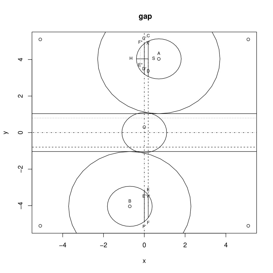 Figure 1
 Figure 2
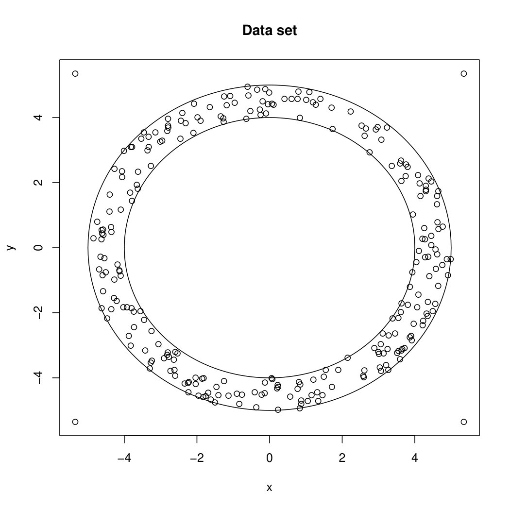 Figure 3
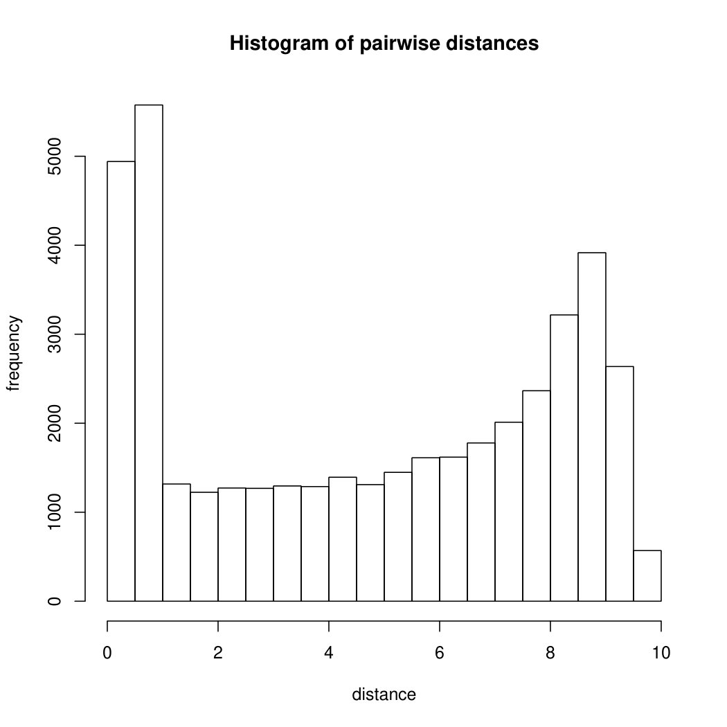 Figure 4
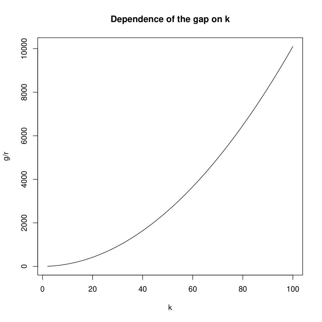 Figure 5
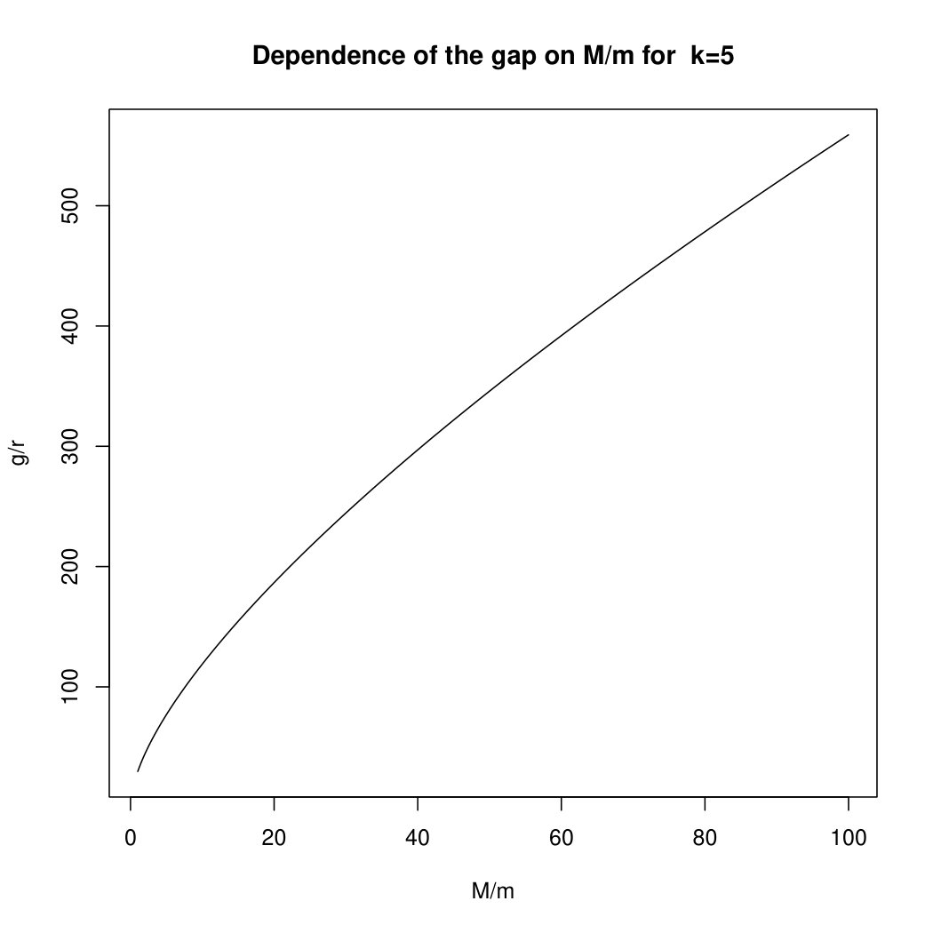 Figure 6
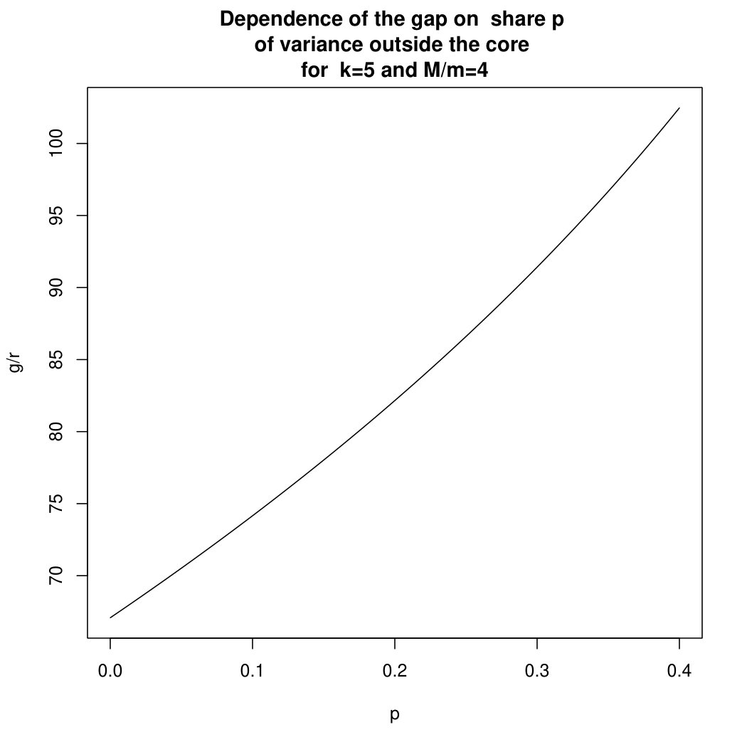 Figure 7
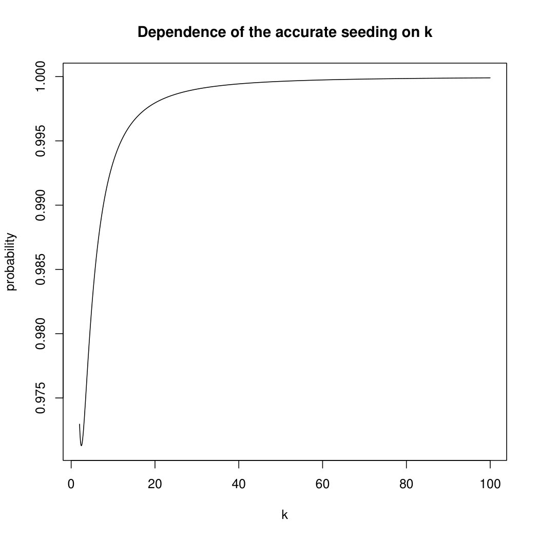 Figure 8
 Figure 9
 Figure 10
| 15 , 9 | 480 , 9 | 720 , 9 | 960 , 9 | |
|---|---|---|---|---|
| Hartigan-Wong 1x | 0 0 | 961.3 8.8 | 974.3 3.2 | 980.9 4.9 |
| 1000 execs in s / relQ | 0.32 / 1 | 0.57 / 1.07 | 0.67 / 1 | 0.79 / 1 |
| Lloyd 1x | 1.7 3.6 | 962.5 5.6 | 974.1 4.9 | 980.4 4.5 |
| 1000 execs in s / relQ | 0.31 / 1.01 | 0.63 / 1.08 | 0.71 / 1.01 | 0.79 / 1.01 |
| Forgy 1x | 0.8 1.8 | 963.3 6.5 | 975.3 3.7 | 980.9 4.6 |
| 1000 execs in s / relQ | 0.3 / 1.01 | 0.63 / 1.08 | 0.71 / 1.01 | 0.79 / 1.01 |
| MacQueen 1x | 1.2 3.2 | 961.8 4.6 | 973.1 5.2 | 982.9 5.9 |
| 1000 execs in s / relQ | 0.31 / 1.01 | 0.54 / 1.07 | 0.64 / 1.01 | 0.72 / 1 |
| Hartigan-Wong 10x | 0 0 | 680.9 25.2 | 1000 0 | 1000 0 |
| 1000 execs in s / relQ | 0.81 / 1 | 7.23 / 1.05 | 10.24 / 1 | 13.42 / 1 |
| Lloyd 10x | 0 0 | 678.6 10.1 | 1000 0 | 1000 0 |
| 1000 execs in s / relQ | 0.72 / 1 | 7.92 / 1.05 | 10.73 / 1 | 13.6 / 1 |
| Forgy 10x | 0 0 | 666.7 14.2 | 1000 0 | 1000 0 |
| 1000 execs in s / relQ | 0.72 / 1 | 7.94 / 1.05 | 10.73 / 1 | 13.52 / 1 |
| MacQueen 10x | 0 0 | 677.2 12 | 1000 0 | 1000 0 |
| 1000 execs in s / relQ | 0.73 / 1 | 7.15 / 1.05 | 9.99 / 1 | 12.92 / 1 |
| Hartigan-Wong 20x | 0 0 | 457.5 14 | 1000 0 | 1000 0 |
| 1000 execs in s / relQ | 1.08 / 1 | 8.75 / 1.03 | 12.63 / 1 | 16.59 / 1 |
| Lloyd 20x | 0 0 | 451.6 9.5 | 1000 0 | 1000 0 |
| 1000 execs in s / relQ | 0.9 / 1 | 9.96 / 1.03 | 13.58 / 1 | 16.79 / 1 |
| Forgy 20x | 0 0 | 457.8 12.4 | 1000 0 | 1000 0 |
| 1000 execs in s / relQ | 0.9 / 1 | 9.95 / 1.03 | 13.44 / 1 | 16.78 / 1 |
| MacQueen 20x | 0 0 | 452.6 14.7 | 1000 0 | 1000 0 |
| 1000 execs in s / relQ | 0.89 / 1 | 8.54 / 1.03 | 12.11 / 1 | 15.69 / 1 |
| cmeans Fuzzy | 0 0 | 973.7 7.9 | 995.4 6.6 | 1000 0 |
| 1000 execs in s / relQ | 0.67 / 1 | 5.37 / 1.09 | 7.37 / 1.02 | 9.43 / 1.02 |
| ufcl Fuzzy | 235.5 59.6 | 964.4 8.9 | 976.8 6.5 | 981.3 5.4 |
| 1000 execs in s / relQ | 0.8 / 1.52 | 6.3 / 1.14 | 8.79 / 1.06 | 11.22 / 1.05 |
| single link | 0 0 | 0 0 | 0 0 | 0 0 |
| 1000 execs in s / relQ | 0.2 / 1 | 13.76 / 1 | 34.39 / 1.06 | 49.01 / 1.15 |
| kmeans++ | 0 0 | 734.7 17 | 811 11.5 | 844 12.5 |
| 1000 execs in s / relQ | 1.14 / 1 | 16.01 / 1.05 | 22.53 / 1.01 | 28.77 / 1.02 |
| kmeans++ 2x | 0 0 | 544.7 28.2 | 959.3 6.1 | 976.9 4.6 |
| 1000 execs in s / relQ | 2.26 / 1 | 31.96 / 1.04 | 44.38 / 1 | 57.49 / 1 |
| Dataset | Errors | WC disc. | WC not disc. | |||
|---|---|---|---|---|---|---|
| -means | -means++ | cc | wc | cc | wc | |
| 0 | 0 | 0 | 0 | 100 | 0 | |
| 0 | 0 | 0 | 0 | 100 | 0 | |
| 38 | 0 | 0 | 0 | 100 | 0 | |
| 26 | 0 | 0 | 0 | 100 | 0 | |
| 74 | 0 | 0 | 0 | 100 | 0 | |
| 66 | 0 | 0 | 0 | 100 | 0 | |
| 0 | 0 | 0 | 0 | 100 | 0 | |
| 0 | 0 | 0 | 0 | 100 | 0 | |
| 50 | 2 | 0 | 0 | 98 | 2 | |
| 37 | 0 | 0 | 0 | 100 | 0 | |
| 78 | 0 | 0 | 0 | 100 | 0 | |
| 73 | 0 | 0 | 0 | 100 | 0 | |
| 0 | 0 | 0 | 0 | 100 | 0 | |
| 0 | 0 | 0 | 0 | 100 | 0 | |
| 41 | 1 | 0 | 0 | 99 | 1 | |
| 29 | 1 | 0 | 0 | 99 | 1 | |
| 74 | 0 | 0 | 0 | 100 | 0 | |
| 78 | 0 | 0 | 0 | 100 | 0 | |
| 0 | 0 | 100 | 0 | 0 | 0 | |
| 0 | 0 | 100 | 0 | 0 | 0 | |
| 41 | 0 | 100 | 0 | 0 | 0 | |
| 39 | 0 | 100 | 0 | 0 | 0 | |
| 80 | 0 | 100 | 0 | 0 | 0 | |
| 80 | 0 | 100 | 0 | 0 | 0 | |
| 0 | 0 | 100 | 0 | 0 | 0 | |
| 0 | 0 | 100 | 0 | 0 | 0 | |
| 43 | 0 | 100 | 0 | 0 | 0 | |
| 38 | 0 | 100 | 0 | 0 | 0 | |
| 80 | 0 | 100 | 0 | 0 | 0 | |
| 75 | 0 | 100 | 0 | 0 | 0 | |
| 0 | 0 | 100 | 0 | 0 | 0 | |
| 0 | 0 | 100 | 0 | 0 | 0 | |
| 33 | 1 | 99 | 0 | 0 | 1 | |
| 33 | 0 | 100 | 0 | 0 | 0 | |
| 75 | 0 | 100 | 0 | 0 | 0 | |
| 79 | 0 | 100 | 0 | 0 | 0 | |
| Dataset | gap type | clusters | Errors | WC disc. | WC not disc. | ||||
| -means | -means++ | cc | wc | cc | wc | ||||
| DNase | orig | 2 | 0 | 69 | 39 | 0 | 0 | 61 | 39 |
| DNase | orig | 2 | 0.1 | 59 | 38 | 0 | 0 | 62 | 38 |
| DNase | g/2 | 2 | 0 | 0 | 0 | 0 | 0 | 100 | 0 |
| DNase | g/2 | 2 | 0.1 | 0 | 0 | 0 | 0 | 100 | 0 |
| DNase | g | 2 | 0 | 0 | 0 | 100 | 0 | 0 | 0 |
| DNase | g | 2 | 0.1 | 0 | 0 | 100 | 0 | 0 | 0 |
| DNase | 2g | 2 | 0 | 0 | 0 | 100 | 0 | 0 | 0 |
| DNase | 2g | 2 | 0.1 | 0 | 0 | 100 | 0 | 0 | 0 |
| DNase | orig | 3 | 0 | 81 | 25 | 0 | 0 | 75 | 25 |
| DNase | orig | 3 | 0.1 | 80 | 28 | 0 | 0 | 72 | 28 |
| DNase | g/2 | 3 | 0 | 63 | 1 | 0 | 0 | 99 | 1 |
| DNase | g/2 | 3 | 0.1 | 59 | 1 | 0 | 0 | 99 | 1 |
| DNase | g | 3 | 0 | 58 | 0 | 100 | 0 | 0 | 0 |
| DNase | g | 3 | 0.1 | 51 | 0 | 100 | 0 | 0 | 0 |
| DNase | 2g | 3 | 0 | 50 | 0 | 100 | 0 | 0 | 0 |
| DNase | 2g | 3 | 0.1 | 49 | 0 | 100 | 0 | 0 | 0 |
| DNase | orig | 5 | 0 | 75 | 35 | 0 | 0 | 65 | 35 |
| DNase | orig | 5 | 0.1 | 79 | 30 | 0 | 0 | 70 | 30 |
| DNase | g/2 | 5 | 0 | 84 | 0 | 0 | 0 | 100 | 0 |
| DNase | g/2 | 5 | 0.1 | 86 | 0 | 0 | 0 | 100 | 0 |
| DNase | g | 5 | 0 | 80 | 0 | 100 | 0 | 0 | 0 |
| DNase | g | 5 | 0.1 | 79 | 0 | 100 | 0 | 0 | 0 |
| DNase | 2g | 5 | 0 | 83 | 0 | 100 | 0 | 0 | 0 |
| DNase | 2g | 5 | 0.1 | 81 | 0 | 100 | 0 | 0 | 0 |
| iris | orig | 2 | 0 | 0 | 0 | 0 | 0 | 100 | 0 |
| iris | orig | 2 | 0.1 | 0 | 0 | 0 | 0 | 100 | 0 |
| iris | g/2 | 2 | 0 | 0 | 0 | 0 | 0 | 100 | 0 |
| iris | g/2 | 2 | 0.1 | 0 | 0 | 0 | 0 | 100 | 0 |
| iris | g | 2 | 0 | 0 | 0 | 100 | 0 | 0 | 0 |
| iris | g | 2 | 0.1 | 0 | 0 | 100 | 0 | 0 | 0 |
| iris | 2g | 2 | 0 | 0 | 0 | 100 | 0 | 0 | 0 |
| iris | 2g | 2 | 0.1 | 0 | 0 | 100 | 0 | 0 | 0 |
| iris | orig | 3 | 0 | 19 | 17 | 0 | 0 | 83 | 17 |
| iris | orig | 3 | 0.1 | 23 | 15 | 0 | 0 | 85 | 15 |
| iris | g/2 | 3 | 0 | 35 | 0 | 0 | 0 | 100 | 0 |
| 2 | 4 | 8 | 16 | |
|---|---|---|---|---|
| Hartigan-Wong 1x | 0 0 | 583 158.5 | 938.3 18.7 | 999.4 0.8 |
| 1000 execs in s / relQ | 0.24 / 1 | 0.3 / 701.98 | 0.44 / 54638.17 | 0.68 / 3276669.6 |
| Lloyd 1x | 0 0 | 655.8 78.2 | 952.7 9.4 | 999.7 0.5 |
| 1000 execs in s / relQ | 0.23 / 1 | 0.29 / 1056.44 | 0.43 / 71083.66 | 0.66 / 4201145 |
| Forgy 1x | 0 0 | 645 75.3 | 950.1 8.1 | 999.9 0.3 |
| 1000 execs in s / relQ | 0.23 / 1 | 0.28 / 1112.96 | 0.43 / 71431.91 | 0.66 / 4175279.99 |
| MacQueen 1x | 0 0 | 642.5 64.2 | 949.9 14.7 | 999.6 0.7 |
| 1000 execs in s / relQ | 0.23 / 1 | 0.28 / 1109.83 | 0.43 / 73197.95 | 0.66 / 4131048.66 |
| Hartigan-Wong 10x | 0 0 | 13 10.4 | 540.9 107.6 | 991.5 10.7 |
| 1000 execs in s / relQ | 0.58 / 1 | 0.61 / 7.26 | 0.99 / 4419.42 | 1.38 / 816542.71 |
| Lloyd 10x | 0 0 | 18.8 16.9 | 621.4 55.9 | 995.2 4.6 |
| 1000 execs in s / relQ | 0.51 / 1 | 0.55 / 9.83 | 0.92 / 6123.88 | 1.27 / 1063785.95 |
| Forgy 10x | 0 0 | 20.8 15.4 | 613.9 58.5 | 996.2 2.1 |
| 1000 execs in s / relQ | 0.51 / 1 | 0.55 / 11.67 | 0.92 / 5976.84 | 1.27 / 1059280.68 |
| MacQueen 10x | 0 0 | 16.2 11.9 | 616.8 68.3 | 996.1 4.4 |
| 1000 execs in s / relQ | 0.51 / 1 | 0.53 / 9.28 | 0.87 / 5611.13 | 1.24 / 1044377.39 |
| Hartigan-Wong 20x | 0 0 | 0 0 | 281.8 101.9 | 986 17.2 |
| 1000 execs in s / relQ | 0.76 / 1 | 0.83 / 1 | 1.28 / 1681.53 | 1.78 / 536122.93 |
| Lloyd 20x | 0 0 | 0.4 0.7 | 385.6 66.5 | 992.8 6.3 |
| 1000 execs in s / relQ | 0.63 / 1 | 0.72 / 1.13 | 1.14 / 2597.6 | 1.58 / 693511.33 |
| Forgy 20x | 0 0 | 0.8 1 | 389.2 62.2 | 992.6 6.5 |
| 1000 execs in s / relQ | 0.63 / 1 | 0.71 / 1.37 | 1.14 / 2670.53 | 1.58 / 680391.36 |
| MacQueen 20x | 0 0 | 0.7 0.8 | 381.4 91.3 | 992.7 6.3 |
| 1000 execs in s / relQ | 0.63 / 1 | 0.66 / 1.37 | 1.06 / 2374.48 | 1.52 / 695009 |
| cmeans Fuzzy | 0 0 | 163 184.5 | 40 63.3 | 35.1 67.3 |
| 1000 execs in s / relQ | 0.48 / 1 | 0.56 / 48.39 | 1.02 / 148.2 | 2.05 / 1213.9 |
| ufcl Fuzzy | 7.8 6.4 | 725 62 | 971.4 7.5 | 999.8 0.4 |
| 1000 execs in s / relQ | 0.56 / 1.14 | 0.68 / 1646.94 | 1.51 / 109702.3 | 3.03 / 5599855.51 |
| single link | 0 0 | 0 0 | 0 0 | 0 0 |
| 1000 execs in s / relQ | 0.15 / 1 | 0.18 / 1 | 0.33 / 1 | 0.56 / 1 |
| kmeans++ | 0 0 | 2.1 1.6 | 0.2 0.4 | 0 0 |
| 1000 execs in s / relQ | 0.78 / 1 | 1.78 / 1.99 | 9.4 / 1.55 | 33.43 / 1 |
| kmeans++ 2x | 0 0 | 0 0 | 0 0 | 0 0 |
| 1000 execs in s / relQ | 1.51 / 1 | 3.53 / 1 | 18.76 / 1 | 66.45 / 1 |
| 2 | 4 | 8 | 16 | |
|---|---|---|---|---|
| Hartigan-Wong 1x | 718.9 65.5 | 695.8 46 | 748.9 43.2 | 750.8 28.7 |
| 1000 execs in s / relQ | 0.34 / 1762.09 | 0.42 / 749.98 | 0.59 / 474.19 | 0.92 / 447.61 |
| Lloyd 1x | 741.8 59.9 | 721.2 31.9 | 779.8 35.2 | 764.7 14.2 |
| 1000 execs in s / relQ | 0.34 / 2108.83 | 0.41 / 860.33 | 0.57 / 520.88 | 0.9 / 470.34 |
| Forgy 1x | 742.5 52.2 | 718.5 28.7 | 773.6 41.9 | 756.3 16.7 |
| 1000 execs in s / relQ | 0.33 / 2116.47 | 0.41 / 844.73 | 0.57 / 517.54 | 0.89 / 467.36 |
| MacQueen 1x | 747 47.3 | 716.2 38.5 | 765.4 46.7 | 751.2 22.3 |
| 1000 execs in s / relQ | 0.34 / 2173.94 | 0.41 / 831 | 0.57 / 503.37 | 0.9 / 459.45 |
| Hartigan-Wong 10x | 45 33.8 | 35 21 | 61.3 26.4 | 52.9 13.6 |
| 1000 execs in s / relQ | 0.77 / 28.8 | 0.92 / 14.86 | 1.28 / 18.92 | 2.11 / 21.8 |
| Lloyd 10x | 57.1 37 | 37.2 14.4 | 86 41.6 | 63.4 14.8 |
| 1000 execs in s / relQ | 0.67 / 35.61 | 0.85 / 15.55 | 1.21 / 26.3 | 2 / 26.12 |
| Forgy 10x | 56.7 35 | 38.7 15.2 | 86.1 47.1 | 63.3 12.5 |
| 1000 execs in s / relQ | 0.68 / 35.61 | 0.85 / 16.23 | 1.22 / 26.04 | 2.01 / 26.02 |
| MacQueen 10x | 55.4 40.6 | 41.7 17.7 | 85.5 49.9 | 63.1 11.6 |
| 1000 execs in s / relQ | 0.67 / 34.85 | 0.82 / 17.41 | 1.18 / 25.78 | 2 / 25.96 |
| Hartigan-Wong 20x | 3.7 4.1 | 0.8 1.3 | 3.5 3.5 | 4.2 2.8 |
| 1000 execs in s / relQ | 1 / 3.29 | 1.16 / 1.33 | 1.54 / 1.98 | 2.42 / 2.63 |
| Lloyd 20x | 4.1 4 | 1.9 1.8 | 10.1 9.5 | 3.5 1.7 |
| 1000 execs in s / relQ | 0.84 / 3.28 | 1.03 / 1.73 | 1.42 / 3.79 | 2.25 / 2.41 |
| Forgy 20x | 4.4 6.9 | 2 1.9 | 9.9 12.3 | 4.3 2.5 |
| 1000 execs in s / relQ | 0.84 / 3.41 | 1.03 / 1.75 | 1.42 / 3.68 | 2.25 / 2.67 |
| MacQueen 20x | 4.8 5.4 | 2.3 2.5 | 8.6 9.2 | 3.2 1.9 |
| 1000 execs in s / relQ | 0.82 / 3.85 | 0.98 / 1.83 | 1.36 / 3.42 | 2.21 / 2.27 |
| cmeans Fuzzy | 155 159.3 | 16 35.3 | 19.2 60.7 | 0 0 |
| 1000 execs in s / relQ | 0.71 / 101.05 | 0.78 / 7.21 | 0.95 / 6.14 | 1.33 / 1 |
| ufcl Fuzzy | 800.7 37.8 | 797.8 28.4 | 867.8 21.9 | 883.5 20.3 |
| 1000 execs in s / relQ | 0.92 / 5952.77 | 1.1 / 1097.38 | 1.57 / 649.79 | 2.69 / 522.86 |
| single link | 0 0 | 0 0 | 0 0 | 0 0 |
| 1000 execs in s / relQ | 0.24 / 1 | 0.29 / 1 | 0.43 / 1 | 0.7 / 1 |
| kmeans++ | 1.2 0.9 | 1.9 1.9 | 4.8 3.6 | 2.7 1.7 |
| 1000 execs in s / relQ | 3.45 / 1.75 | 3.34 / 2.06 | 3.69 / 2.54 | 4.52 / 2.17 |
| kmeans++ 2x | 0 0 | 0 0 | 0 0 | 0 0 |
| 1000 execs in s / relQ | 6.83 / 1 | 6.58 / 1 | 7.09 / 1 | 8.53 / 1 |
| 15 , 9 | 30 , 9 | 60 , 9 | 120 , 9 | |
|---|---|---|---|---|
| Hartigan-Wong 1x | 723.7 43.5 | 801 58.1 | 762.9 49.4 | 736.1 76.4 |
| 1000 execs in s / relQ | 0.36 / 6216.55 | 0.37 / 10441.43 | 0.41 / 2427.55 | 0.45 / 5018.41 |
| Lloyd 1x | 730.4 50.7 | 804.9 67.4 | 777.3 54.6 | 733.8 88.3 |
| 1000 execs in s / relQ | 0.35 / 7085.08 | 0.36 / 11054.14 | 0.4 / 2456.29 | 0.45 / 5112.28 |
| Forgy 1x | 731.3 50.2 | 809.8 67 | 775.2 57.9 | 748.9 81 |
| 1000 execs in s / relQ | 0.34 / 7404.61 | 0.36 / 10798.16 | 0.41 / 2508.64 | 0.45 / 5033.54 |
| MacQueen 1x | 726.8 44.9 | 809 70.7 | 777.7 53 | 741.3 88.3 |
| 1000 execs in s / relQ | 0.35 / 7206.3 | 0.35 / 11617.69 | 0.39 / 2508.61 | 0.43 / 4884.21 |
| Hartigan-Wong 10x | 44.4 26.7 | 126.3 73.5 | 83.8 52 | 69 47.1 |
| 1000 execs in s / relQ | 1.1 / 24.72 | 1.32 / 119.48 | 2.56 / 59.89 | 3.79 / 47.41 |
| Lloyd 10x | 46.6 29.8 | 138.8 88.7 | 93.2 55.9 | 75.2 51.4 |
| 1000 execs in s / relQ | 1.01 / 25.78 | 1.23 / 114.56 | 2.57 / 63.23 | 3.83 / 51.64 |
| Forgy 10x | 48.7 34.1 | 143.5 91.1 | 95 56.1 | 69.9 49.1 |
| 1000 execs in s / relQ | 1.01 / 27.43 | 1.22 / 149.46 | 2.56 / 64.55 | 3.82 / 48.17 |
| MacQueen 10x | 46.5 25.4 | 138.6 87.6 | 82.5 52.4 | 66.9 46.8 |
| 1000 execs in s / relQ | 0.99 / 26.53 | 1.19 / 142.97 | 2.38 / 57.64 | 3.57 / 46.12 |
| Hartigan-Wong 20x | 2.2 3.6 | 17.2 15.7 | 8.7 11.2 | 6.3 6.8 |
| 1000 execs in s / relQ | 1.38 / 2.15 | 1.63 / 9.17 | 3.04 / 6.78 | 4.45 / 4.91 |
| Lloyd 20x | 3.5 4.4 | 26.3 27.5 | 11 13.7 | 8.6 10 |
| 1000 execs in s / relQ | 1.19 / 2.81 | 1.45 / 16.83 | 3.08 / 7.88 | 4.58 / 6.92 |
| Forgy 20x | 3.2 4 | 27.7 28.1 | 11.2 10.3 | 7.9 8.4 |
| 1000 execs in s / relQ | 1.19 / 2.62 | 1.45 / 13.49 | 3.08 / 7.91 | 4.57 / 6.1 |
| MacQueen 20x | 3.8 6.1 | 23.7 24.6 | 9.8 12.4 | 7.4 8.1 |
| 1000 execs in s / relQ | 1.17 / 2.89 | 1.4 / 11.74 | 2.72 / 7.28 | 4.07 / 5.74 |
| cmeans Fuzzy | 100 120.3 | 119.2 113.8 | 46.9 51.9 | 59 83 |
| 1000 execs in s / relQ | 0.99 / 51.88 | 1.15 / 64.07 | 2.09 / 35.43 | 3.07 / 48.86 |
| ufcl Fuzzy | 810.6 19.5 | 866.6 23.3 | 828.8 31.9 | 846.4 25.1 |
| 1000 execs in s / relQ | 1.48 / 15995.33 | 1.83 / 14805.01 | 3.88 / 3690.75 | 5.91 / 14135.23 |
| single link | 0 0 | 0 0 | 0 0 | 0 0 |
| 1000 execs in s / relQ | 0.34 / 1 | 0.44 / 1 | 1.47 / 1 | 3.4 / 1 |
| kmeans++ | 1.3 1.1 | 1.3 1.1 | 1.4 1.2 | 1.1 1.4 |
| 1000 execs in s / relQ | 7.25 / 1.7 | 9.59 / 1.63 | 23.52 / 2.69 | 37.31 / 1.69 |
| kmeans++ 2x | 0 0 | 0 0 | 0 0 | 0 0 |
| 1000 execs in s / relQ | 14.48 / 1 | 19.12 / 1 | 47.03 / 1 | 74.88 / 1 |
| 15 , 9 | 30 , 18 | 60 , 36 | 120 , 72 | |
|---|---|---|---|---|
| Hartigan-Wong 1x | 714.5 55.3 | 726.7 41 | 751.6 35.1 | 739.4 48.6 |
| 1000 execs in s / relQ | 0.36 / 2222.82 | 0.38 / 9506.9 | 0.4 / 2452.25 | 0.48 / 1017.77 |
| Lloyd 1x | 731.6 39.9 | 737.9 34.2 | 743.6 42.8 | 733.5 34.2 |
| 1000 execs in s / relQ | 0.35 / 2542.88 | 0.37 / 9537.46 | 0.4 / 2376.59 | 0.48 / 1011.3 |
| Forgy 1x | 725.9 46.8 | 734.9 49 | 756.1 39 | 739.2 36.8 |
| 1000 execs in s / relQ | 0.35 / 2599.24 | 0.37 / 9968.81 | 0.39 / 2606.82 | 0.48 / 1007.41 |
| MacQueen 1x | 736.8 41.3 | 735.2 39.8 | 753 42.5 | 734.5 35.1 |
| 1000 execs in s / relQ | 0.35 / 2547.24 | 0.36 / 9369.12 | 0.38 / 2509.95 | 0.45 / 970.99 |
| Hartigan-Wong 10x | 41.8 25.7 | 48.1 29.8 | 61.1 29.7 | 54.1 32.9 |
| 1000 execs in s / relQ | 1.05 / 37.25 | 1.84 / 28.47 | 2.36 / 39.86 | 4.83 / 19.06 |
| Lloyd 10x | 47.3 32.4 | 53.7 27.2 | 64.8 31.4 | 53.8 30.3 |
| 1000 execs in s / relQ | 0.97 / 40.99 | 1.63 / 31.44 | 2.28 / 42.89 | 4.9 / 18.99 |
| Forgy 10x | 52.6 33.2 | 49.3 26.7 | 64.6 27.4 | 51.3 25.2 |
| 1000 execs in s / relQ | 0.96 / 45.82 | 1.63 / 29.53 | 2.28 / 42.94 | 4.91 / 18.29 |
| MacQueen 10x | 50.2 31.2 | 50.5 27 | 65.2 28.9 | 54 29.2 |
| 1000 execs in s / relQ | 0.95 / 44.05 | 1.57 / 29.42 | 2.19 / 42.68 | 4.59 / 19.07 |
| Hartigan-Wong 20x | 2.7 3.5 | 3.3 3.3 | 3.7 2.8 | 2.5 2.3 |
| 1000 execs in s / relQ | 1.33 / 3.24 | 2.07 / 2.84 | 2.81 / 3.58 | 5.64 / 1.82 |
| Lloyd 20x | 4.5 4.9 | 2.9 3 | 5 3.9 | 2.3 2.9 |
| 1000 execs in s / relQ | 1.16 / 4.61 | 1.91 / 2.61 | 2.67 / 4.13 | 5.81 / 1.78 |
| Forgy 20x | 4 4.5 | 3 3 | 4.6 3.9 | 3.1 3.1 |
| 1000 execs in s / relQ | 1.16 / 4.22 | 1.91 / 2.66 | 2.66 / 3.87 | 5.82 / 2.06 |
| MacQueen 20x | 2.7 3.3 | 2.9 2.9 | 3.8 3.8 | 2.3 2.5 |
| 1000 execs in s / relQ | 1.11 / 3.2 | 1.81 / 2.61 | 2.51 / 3.33 | 5.2 / 1.75 |
| cmeans Fuzzy | 23.9 33.9 | 70.7 117.4 | 82.4 87.2 | 55.3 50.3 |
| 1000 execs in s / relQ | 0.92 / 22.94 | 1.45 / 39.24 | 2 / 62.64 | 3.94 / 18.83 |
| ufcl Fuzzy | 813.5 24.8 | 808.6 15.9 | 805.2 18.5 | 825.3 20.2 |
| 1000 execs in s / relQ | 1.39 / 4980.44 | 2.5 / 12524.72 | 3.57 / 5516.03 | 7.71 / 1798.34 |
| single link | 0 0 | 0 0 | 0 0 | 0 0 |
| 1000 execs in s / relQ | 0.32 / 1 | 0.68 / 1 | 1.27 / 1 | 6.13 / 1 |
| kmeans++ | 0.8 1.3 | 0.6 0.8 | 0.6 0.7 | 1.9 1.3 |
| 1000 execs in s / relQ | 6.57 / 1.61 | 14.13 / 1.32 | 21.48 / 1.43 | 49.4 / 1.73 |
| kmeans++ 2x | 0 0 | 0 0 | 0 0 | 0 0 |
| 1000 execs in s / relQ | 13.09 / 1 | 28.24 / 1 | 42.93 / 1 | 98.78 / 1 |
| 1 | 2 | 4 | 8 | |
|---|---|---|---|---|
| Hartigan-Wong 1x | 727.8 47.5 | 713.8 35.1 | 697.3 69.2 | 663.3 42.7 |
| 1000 execs in s / relQ | 0.36 / 1312.52 | 0.36 / 710.88 | 0.37 / 133.68 | 0.36 / 55.72 |
| Lloyd 1x | 735.7 42.4 | 728 35.7 | 717.7 29.6 | 690.8 32.5 |
| 1000 execs in s / relQ | 0.35 / 1469.84 | 0.35 / 720.23 | 0.37 / 143.39 | 0.36 / 61.49 |
| Forgy 1x | 733.1 39.7 | 729.8 27.5 | 721.2 39.9 | 689.2 22.3 |
| 1000 execs in s / relQ | 0.35 / 1421.55 | 0.34 / 715.94 | 0.37 / 145.41 | 0.35 / 63.16 |
| MacQueen 1x | 736.1 43.4 | 717.4 35.9 | 711.9 51.5 | 684.9 29.1 |
| 1000 execs in s / relQ | 0.35 / 1440.8 | 0.34 / 764.85 | 0.36 / 140.76 | 0.34 / 63.32 |
| Hartigan-Wong 10x | 52.6 25.3 | 36.7 14.8 | 31.4 21.2 | 20.9 12.3 |
| 1000 execs in s / relQ | 1.01 / 22.4 | 0.98 / 5.98 | 1.06 / 2.18 | 1 / 1.23 |
| Lloyd 10x | 49.5 22 | 39.7 17.1 | 41.4 25.1 | 24.8 4.7 |
| 1000 execs in s / relQ | 0.92 / 21.14 | 0.91 / 5.92 | 0.99 / 2.62 | 0.96 / 1.29 |
| Forgy 10x | 51.4 22.1 | 42.6 14.9 | 42.3 20.6 | 26.6 8.9 |
| 1000 execs in s / relQ | 0.93 / 22.14 | 0.91 / 6.52 | 1 / 2.65 | 0.96 / 1.3 |
| MacQueen 10x | 50.4 25.9 | 39.2 17.6 | 40.9 20.5 | 20.7 6.9 |
| 1000 execs in s / relQ | 0.9 / 21.57 | 0.88 / 5.86 | 0.95 / 2.61 | 0.89 / 1.24 |
| Hartigan-Wong 20x | 3.4 2.6 | 1.6 1.9 | 1.7 2.9 | 0.9 1.5 |
| 1000 execs in s / relQ | 1.27 / 2.32 | 1.25 / 1.19 | 1.35 / 1.06 | 1.27 / 1.01 |
| Lloyd 20x | 2.8 2.7 | 1.8 1.5 | 1.7 2.2 | 0.7 0.8 |
| 1000 execs in s / relQ | 1.11 / 2.09 | 1.11 / 1.23 | 1.22 / 1.06 | 1.21 / 1.01 |
| Forgy 20x | 3.1 2.4 | 3.4 1.6 | 2.8 3.2 | 0.9 0.9 |
| 1000 execs in s / relQ | 1.11 / 2.19 | 1.12 / 1.42 | 1.21 / 1.11 | 1.21 / 1.01 |
| MacQueen 20x | 2.4 2.5 | 2.2 2.5 | 1.1 1.9 | 0.3 0.5 |
| 1000 execs in s / relQ | 1.07 / 1.92 | 1.05 / 1.26 | 1.13 / 1.04 | 1.06 / 1 |
| cmeans Fuzzy | 57.2 67.9 | 159.8 153.7 | 171.5 109.1 | 247.8 128.8 |
| 1000 execs in s / relQ | 0.89 / 25.26 | 0.9 / 26.38 | 0.98 / 7.94 | 0.93 / 4.18 |
| ufcl Fuzzy | 800.8 29.2 | 801.4 16.7 | 853.2 34.1 | 901.3 36.2 |
| 1000 execs in s / relQ | 1.32 / 1989.2 | 1.3 / 1645.95 | 1.4 / 289.28 | 1.31 / 105.34 |
| single link | 0 0 | 0 0 | 0 0 | 0 0 |
| 1000 execs in s / relQ | 0.3 / 1 | 0.3 / 1 | 0.32 / 1 | 0.3 / 1 |
| kmeans++ | 1.6 1.1 | 4.9 3.2 | 12.1 6.5 | 47.5 19.4 |
| 1000 execs in s / relQ | 6.1 / 1.68 | 5.95 / 1.66 | 6.54 / 1.49 | 6.03 / 1.57 |
| kmeans++ 2x | 0 0 | 0 0 | 0 0 | 3.2 2.9 |
| 1000 execs in s / relQ | 12.12 / 1 | 11.82 / 1 | 13.08 / 1 | 11.96 / 1.03 |
| 2 | 4 | 8 | 16 | |
|---|---|---|---|---|
| Hartigan-Wong 1x | 0 0 | 531 93.8 | 941.3 11.5 | 999.3 0.8 |
| 1000 execs in s / relQ | 0.25 / 1 | 0.33 / 1484.76 | 0.49 / 494624.56 | 0.81 / 52872221.3 |
| Lloyd 1x | 0 0 | 520.8 97.7 | 942.3 11.7 | 999.4 0.7 |
| 1000 execs in s / relQ | 0.24 / 1 | 0.32 / 1492.16 | 0.48 / 502271.64 | 0.8 / 58530442.16 |
| Forgy 1x | 0 0 | 524.9 81.9 | 940 12.2 | 998.8 1.1 |
| 1000 execs in s / relQ | 0.24 / 1 | 0.32 / 1548 | 0.48 / 520427.63 | 0.8 / 54534626.71 |
| MacQueen 1x | 0 0 | 520.5 82.6 | 945 13.2 | 999.4 0.5 |
| 1000 execs in s / relQ | 0.24 / 1 | 0.32 / 1495.12 | 0.47 / 532067.28 | 0.79 / 57986428.7 |
| Hartigan-Wong 10x | 0 0 | 2.6 2.8 | 541 62.9 | 992.9 2.6 |
| 1000 execs in s / relQ | 0.63 / 1 | 0.93 / 3.41 | 1.54 / 16469.01 | 2.86 / 7858388.63 |
| Lloyd 10x | 0 0 | 3.3 3.1 | 563.2 68.1 | 994.1 3 |
| 1000 execs in s / relQ | 0.56 / 1 | 0.84 / 4.16 | 1.44 / 18712.34 | 2.77 / 8511396.87 |
| Forgy 10x | 0 0 | 3.4 3 | 558.3 71.5 | 993.5 3.5 |
| 1000 execs in s / relQ | 0.56 / 1 | 0.84 / 4.2 | 1.44 / 17368.35 | 2.76 / 8325871.74 |
| MacQueen 10x | 0 0 | 2.9 2.5 | 551.2 59.2 | 992.9 2.7 |
| 1000 execs in s / relQ | 0.56 / 1 | 0.83 / 3.82 | 1.4 / 17832.1 | 2.66 / 8382457.42 |
| Hartigan-Wong 20x | 0 0 | 0 0 | 299.9 66.5 | 986.3 3.9 |
| 1000 execs in s / relQ | 0.84 / 1 | 1.18 / 1 | 1.94 / 4916.09 | 3.61 / 4501700.03 |
| Lloyd 20x | 0 0 | 0 0 | 322.2 69.9 | 987 4.4 |
| 1000 execs in s / relQ | 0.69 / 1 | 1.01 / 1 | 1.74 / 5325.33 | 3.43 / 4989161.44 |
| Forgy 20x | 0 0 | 0.1 0.3 | 318.9 69.3 | 987.4 4.7 |
| 1000 execs in s / relQ | 0.69 / 1 | 1 / 1.09 | 1.74 / 5318.02 | 3.43 / 4869931.56 |
| MacQueen 20x | 0 0 | 0 0 | 308.4 68.3 | 986.3 3.8 |
| 1000 execs in s / relQ | 0.69 / 1 | 0.99 / 1 | 1.65 / 5183.37 | 3.27 / 4810210.65 |
| cmeans Fuzzy | 0 0 | 32.6 43.8 | 64.3 74.2 | 53.7 76.1 |
| 1000 execs in s / relQ | 0.51 / 1 | 0.78 / 36.04 | 1.67 / 857.64 | 5.06 / 14553.66 |
| ufcl Fuzzy | 10.3 8.1 | 637.2 22.1 | 958.8 8.6 | 999.4 1 |
| 1000 execs in s / relQ | 0.61 / 1.27 | 1.1 / 3550.22 | 2.78 / 899036.18 | 8.83 / 104163506.23 |
| single link | 0 0 | 0 0 | 0 0 | 0 0 |
| 1000 execs in s / relQ | 0.16 / 1 | 0.27 / 1 | 0.57 / 1 | 1.48 / 1 |
| kmeans++ | 0 0 | 0.6 0.7 | 0.2 0.4 | 0 0 |
| 1000 execs in s / relQ | 0.89 / 1 | 4.1 / 1.81 | 21.14 / 3.59 | 115.57 / 1 |
| kmeans++ 2x | 0 0 | 0 0 | 0 0 | 0 0 |
| 1000 execs in s / relQ | 1.77 / 1 | 8.19 / 1 | 42.03 / 1 | 230.99 / 1 |
| 2 | 4 | 8 | 16 | |
|---|---|---|---|---|
| Hartigan-Wong 1x | 707.1 50.5 | 744.6 38.5 | 753.3 21.4 | 764.7 19.4 |
| 1000 execs in s / relQ | 0.36 / 8483.66 | 0.45 / 3683.63 | 0.62 / 1761.1 | 0.97 / 2022.89 |
| Lloyd 1x | 717 52.5 | 760.8 39.9 | 753.4 18.8 | 770.1 16.8 |
| 1000 execs in s / relQ | 0.35 / 8896.63 | 0.43 / 3873.14 | 0.61 / 1802.6 | 0.95 / 2088.42 |
| Forgy 1x | 711.6 53.1 | 755.1 36.5 | 756 16.9 | 765.2 25.3 |
| 1000 execs in s / relQ | 0.35 / 8982.63 | 0.43 / 3741.16 | 0.61 / 1795.73 | 0.95 / 2105.67 |
| MacQueen 1x | 720.5 44.3 | 753 35.8 | 748.9 20.4 | 769.5 25 |
| 1000 execs in s / relQ | 0.35 / 8986.52 | 0.43 / 3875.21 | 0.61 / 1797.93 | 0.95 / 2104.26 |
| Hartigan-Wong 10x | 38.9 20.8 | 53.8 24.6 | 59.8 13.3 | 70.7 23.2 |
| 1000 execs in s / relQ | 1.07 / 87.64 | 1.4 / 67.03 | 2.02 / 76.71 | 3.27 / 106.07 |
| Lloyd 10x | 48 23.2 | 65.4 25.9 | 62.8 12.6 | 81.5 24.7 |
| 1000 execs in s / relQ | 0.97 / 106.61 | 1.31 / 81.6 | 1.92 / 81.15 | 3.17 / 122.66 |
| Forgy 10x | 43.9 21.5 | 68.1 26.1 | 64.2 12.5 | 82.4 20.5 |
| 1000 execs in s / relQ | 0.97 / 98.81 | 1.3 / 85.49 | 1.91 / 82.4 | 3.16 / 124.99 |
| MacQueen 10x | 43.6 20.8 | 64.6 23.6 | 64.5 12.1 | 80.5 23.7 |
| 1000 execs in s / relQ | 1.35 / 99.1 | 1.29 / 81.23 | 1.89 / 83.85 | 3.12 / 121.61 |
| Hartigan-Wong 20x | 2.3 2.4 | 3.3 2.7 | 4.2 3.3 | 5.1 3.3 |
| 1000 execs in s / relQ | 1.35 / 5.9 | 1.71 / 4.99 | 2.37 / 6.34 | 3.72 / 8.42 |
| Lloyd 20x | 2.9 2.7 | 4.2 3.5 | 4.3 2.9 | 6.1 3.1 |
| 1000 execs in s / relQ | 1.15 / 7.34 | 1.51 / 6.08 | 2.17 / 6.42 | 3.52 / 10.17 |
| Forgy 20x | 1.6 1.6 | 5.9 3.9 | 3.2 0.9 | 7.5 3.1 |
| 1000 execs in s / relQ | 1.15 / 4.41 | 1.51 / 8.15 | 2.17 / 4.98 | 3.51 / 12.02 |
| MacQueen 20x | 3.4 2.6 | 5.7 3.2 | 2.9 1.7 | 8.2 5.3 |
| 1000 execs in s / relQ | 1.13 / 8.21 | 1.48 / 7.92 | 2.13 / 4.57 | 3.43 / 12.97 |
| cmeans Fuzzy | 41.5 65.6 | 10.6 18 | 0 0 | 0 0 |
| 1000 execs in s / relQ | 0.97 / 92.62 | 1.04 / 14.1 | 1.21 / 1 | 1.58 / 1 |
| ufcl Fuzzy | 784.6 20.6 | 805.6 15.7 | 800.3 19.4 | 814.9 13.6 |
| 1000 execs in s / relQ | 1.46 / 27141.38 | 1.86 / 4984.43 | 2.66 / 1940.95 | 4.39 / 2223.44 |
| single link | 0 0 | 0 0 | 0 0 | 0 0 |
| 1000 execs in s / relQ | 0.33 / 1 | 0.41 / 1 | 0.56 / 1 | 0.87 / 1 |
| kmeans++ | 0.4 0.7 | 0.5 0.7 | 0.7 0.8 | 0.5 0.7 |
| 1000 execs in s / relQ | 6.89 / 2 | 7.21 / 1.64 | 7.44 / 1.96 | 7.98 / 1.8 |
| kmeans++ 2x | 0 0 | 0 0 | 0 0 | 0 0 |
| 1000 execs in s / relQ | 14.03 / 1 | 14.3 / 1 | 14.62 / 1 | 15.45 / 1 |
| 15 , 9 | 30 , 9 | 60 , 9 | 120 , 9 | |
|---|---|---|---|---|
| Hartigan-Wong 1x | 709.6 40.7 | 778.2 20.9 | 789 36.6 | 765.3 42.5 |
| 1000 execs in s / relQ | 0.52 / 9331.26 | 0.51 / 9154.2 | 0.56 / 11397.3 | 0.68 / 58999.38 |
| Lloyd 1x | 730.6 38.3 | 781.8 19.6 | 786.1 35.1 | 780.7 49.8 |
| 1000 execs in s / relQ | 0.5 / 10181.63 | 0.49 / 9648.81 | 0.54 / 11275.24 | 0.67 / 58343.78 |
| Forgy 1x | 723.8 38.2 | 786.5 28 | 792.6 37 | 778 42.6 |
| 1000 execs in s / relQ | 0.49 / 10529.17 | 0.49 / 9641 | 0.55 / 11645.35 | 0.68 / 58111.99 |
| MacQueen 1x | 733.6 32.4 | 780.2 24.7 | 784.3 38.6 | 767.7 49.8 |
| 1000 execs in s / relQ | 0.49 / 10804.58 | 0.48 / 10006.28 | 0.53 / 11472.56 | 0.63 / 54103.2 |
| Hartigan-Wong 10x | 38.3 23.1 | 87.6 28.5 | 96.1 57.6 | 89.6 44.1 |
| 1000 execs in s / relQ | 1.63 / 81.12 | 2.15 / 239.35 | 3.04 / 500.28 | 6.44 / 602.73 |
| Lloyd 10x | 48.1 25.7 | 87.2 25 | 96.7 46.4 | 79.1 40.7 |
| 1000 execs in s / relQ | 1.47 / 105.41 | 2.01 / 239.14 | 2.93 / 509.78 | 6.5 / 582.16 |
| Forgy 10x | 47.9 19.8 | 86 25.5 | 102.1 45.6 | 89.9 40.4 |
| 1000 execs in s / relQ | 1.46 / 104.24 | 2 / 233.97 | 2.93 / 546.54 | 6.54 / 653.92 |
| MacQueen 10x | 46.6 22.5 | 95.3 26.4 | 100.8 58.3 | 87 45.5 |
| 1000 execs in s / relQ | 1.42 / 102.86 | 1.96 / 259.02 | 2.8 / 522.96 | 6.13 / 556.78 |
| Hartigan-Wong 20x | 1.6 3.1 | 8.2 5.3 | 12.7 15 | 7.7 6.8 |
| 1000 execs in s / relQ | 1.99 / 4.26 | 2.62 / 23.24 | 3.62 / 65.01 | 7.55 / 35.06 |
| Lloyd 20x | 2.7 3.5 | 7 4.1 | 13.3 15.1 | 10 8.3 |
| 1000 execs in s / relQ | 1.74 / 6.54 | 2.35 / 19.65 | 3.41 / 67.85 | 7.72 / 59.9 |
| Forgy 20x | 2.6 3.3 | 7.6 4.1 | 12.7 14.5 | 8.2 5.9 |
| 1000 execs in s / relQ | 1.74 / 6.32 | 2.34 / 21.5 | 3.42 / 66.49 | 7.81 / 39.85 |
| MacQueen 20x | 3.2 2.9 | 8.2 5.6 | 12.9 14.1 | 9.2 7.1 |
| 1000 execs in s / relQ | 1.71 / 7.68 | 2.27 / 22.95 | 3.23 / 66.18 | 6.96 / 42.72 |
| cmeans Fuzzy | 43.1 85.3 | 29.8 59.5 | 4.8 15.2 | 29.9 54.3 |
| 1000 execs in s / relQ | 1.42 / 89.96 | 1.84 / 66.83 | 2.52 / 23.17 | 5.23 / 164.93 |
| ufcl Fuzzy | 786.1 26.5 | 815.4 24.5 | 825.9 32.1 | 830 33.3 |
| 1000 execs in s / relQ | 2.25 / 22096.93 | 3.22 / 13196.22 | 4.73 / 17181.09 | 10.65 / 83971.71 |
| single link | 0 0 | 0 0 | 0 0 | 0 0 |
| 1000 execs in s / relQ | 0.49 / 1 | 0.82 / 1 | 1.48 / 1 | 7.58 / 1 |
| kmeans++ | 0.6 0.7 | 0 0 | 0 0 | 0 0 |
| 1000 execs in s / relQ | 10.72 / 2.4 | 17.33 / 1 | 27.18 / 1 | 65.24 / 1 |
| kmeans++ 2x | 0 0 | 0 0 | 0 0 | 0 0 |
| 1000 execs in s / relQ | 21.64 / 1 | 34.62 / 1 | 54.08 / 1 | 129.98 / 1 |
| 15 , 9 | 30 , 18 | 60 , 36 | 120 , 72 | |
|---|---|---|---|---|
| Hartigan-Wong 1x | 739.4 28.1 | 741 44 | 745.7 70 | 713 64.6 |
| 1000 execs in s / relQ | 0.37 / 42678.96 | 0.38 / 20676.98 | 0.42 / 5466.12 | 0.49 / 138752.72 |
| Lloyd 1x | 734.4 28.5 | 741.4 48.9 | 743.5 69.7 | 710.4 70.6 |
| 1000 execs in s / relQ | 0.35 / 46792.33 | 0.37 / 20423.87 | 0.41 / 5537.44 | 0.49 / 151687.77 |
| Forgy 1x | 734.1 34.3 | 745 41.4 | 751.3 74.9 | 713.5 69.7 |
| 1000 execs in s / relQ | 0.35 / 46112.12 | 0.36 / 20150.75 | 0.41 / 5548.93 | 0.49 / 144663.49 |
| MacQueen 1x | 738.8 33.8 | 739.2 49.6 | 743.6 77.5 | 710.9 66.3 |
| 1000 execs in s / relQ | 0.35 / 45493.36 | 0.36 / 19576.95 | 0.4 / 5587.02 | 0.46 / 137172.51 |
| Hartigan-Wong 10x | 49 19.1 | 57 24.6 | 59.9 21.6 | 48.6 33.5 |
| 1000 execs in s / relQ | 1.12 / 145.96 | 1.65 / 191.09 | 2.8 / 192.09 | 5 / 122.97 |
| Lloyd 10x | 54.2 22.3 | 55.4 29 | 64.7 22.2 | 41.3 30.7 |
| 1000 execs in s / relQ | 1.02 / 157.45 | 1.55 / 186.28 | 2.75 / 206.05 | 5.02 / 103.98 |
| Forgy 10x | 56 24.3 | 59.6 27.2 | 66.9 26.2 | 43.9 36.1 |
| 1000 execs in s / relQ | 1.02 / 205.13 | 1.55 / 204.96 | 2.74 / 214.45 | 5.02 / 113.15 |
| MacQueen 10x | 52.1 21.9 | 57.2 28.4 | 62 27.3 | 42.2 29.9 |
| 1000 execs in s / relQ | 1.01 / 147.45 | 1.51 / 190.38 | 2.61 / 199.76 | 4.76 / 106.24 |
| Hartigan-Wong 20x | 2.8 3.2 | 3.4 2.5 | 4.8 3.5 | 2.8 3 |
| 1000 execs in s / relQ | 1.4 / 8.73 | 1.99 / 12.17 | 3.3 / 16.17 | 5.82 / 7.98 |
| Lloyd 20x | 3 2.2 | 4.8 5.8 | 5.5 2.6 | 3.5 4.7 |
| 1000 execs in s / relQ | 1.22 / 9.45 | 1.81 / 17.56 | 3.23 / 18.34 | 5.89 / 9.85 |
| Forgy 20x | 3 3 | 5.6 6.4 | 5.2 3.2 | 2.4 3.5 |
| 1000 execs in s / relQ | 1.22 / 9.35 | 1.81 / 20.08 | 3.22 / 17.34 | 5.9 / 6.94 |
| MacQueen 20x | 3.3 3.9 | 3.4 2.6 | 4.8 2.3 | 2.9 3.7 |
| 1000 execs in s / relQ | 1.19 / 10.02 | 1.74 / 12.45 | 2.98 / 16.03 | 5.39 / 8.23 |
| cmeans Fuzzy | 89.6 106.4 | 46.4 112.3 | 19 36.1 | 122.4 127.9 |
| 1000 execs in s / relQ | 0.98 / 250.43 | 1.38 / 136.32 | 2.22 / 58.89 | 4.13 / 313.25 |
| ufcl Fuzzy | 786 20.1 | 806.5 21.9 | 795.7 20.3 | 801.8 33 |
| 1000 execs in s / relQ | 1.51 / 77257.56 | 2.38 / 33556.99 | 4.29 / 16111.26 | 8 / 232714.84 |
| single link | 0 0 | 0 0 | 0 0 | 0 0 |
| 1000 execs in s / relQ | 0.35 / 1 | 0.66 / 1 | 1.91 / 1 | 7.33 / 1 |
| kmeans++ | 0.2 0.4 | 0.3 0.7 | 0.2 0.4 | 0.6 0.7 |
| 1000 execs in s / relQ | 7.47 / 1.85 | 13.46 / 2.07 | 26.66 / 1.67 | 51.85 / 2.41 |
| kmeans++ 2x | 0 0 | 0 0 | 0 0 | 0 0 |
| 1000 execs in s / relQ | 14.85 / 1 | 26.82 / 1 | 53.17 / 1 | 103.47 / 1 |
| 1 | 2 | 4 | 8 | |
|---|---|---|---|---|
| Hartigan-Wong 1x | 737.8 36.7 | 704.8 62.6 | 712.5 62.9 | 711.6 41.7 |
| 1000 execs in s / relQ | 0.49 / 14832.58 | 0.49 / 1527.1 | 0.47 / 874.07 | 0.47 / 221.09 |
| Lloyd 1x | 744.5 29.1 | 724.8 52.9 | 726.7 53.6 | 731.8 28.8 |
| 1000 execs in s / relQ | 0.48 / 15121.58 | 0.47 / 1830.33 | 0.46 / 923.38 | 0.46 / 246.31 |
| Forgy 1x | 743.1 30 | 717.1 60.7 | 714.1 48.2 | 729.5 42 |
| 1000 execs in s / relQ | 0.48 / 15136.66 | 0.48 / 1764 | 0.46 / 938.35 | 0.46 / 239.11 |
| MacQueen 1x | 736.7 21.8 | 721.8 58.6 | 721.6 57.6 | 727.1 31.7 |
| 1000 execs in s / relQ | 0.48 / 14539.53 | 0.48 / 1824.64 | 0.48 / 946.43 | 0.45 / 235.61 |
| Hartigan-Wong 10x | 50.5 19 | 36.2 17.4 | 39.1 20 | 44.4 17.4 |
| 1000 execs in s / relQ | 1.56 / 99.45 | 1.5 / 22.34 | 1.44 / 6.98 | 1.43 / 3.32 |
| Lloyd 10x | 51.8 14.8 | 43.8 25 | 45.4 28.5 | 49.9 19.2 |
| 1000 execs in s / relQ | 1.41 / 101.54 | 1.39 / 27.1 | 1.32 / 7.92 | 1.34 / 3.57 |
| Forgy 10x | 55.2 15.7 | 42.9 20.1 | 43.3 26.1 | 47.7 20.2 |
| 1000 execs in s / relQ | 1.41 / 108.27 | 1.36 / 26.29 | 1.32 / 7.58 | 1.33 / 3.49 |
| MacQueen 10x | 48.1 19.2 | 39.6 21.8 | 40.5 25.7 | 41.8 19.2 |
| 1000 execs in s / relQ | 1.39 / 94.4 | 1.33 / 24.45 | 1.29 / 7.16 | 1.29 / 3.26 |
| Hartigan-Wong 20x | 1.9 1.6 | 2.4 1.9 | 1.8 2.3 | 2.1 2.1 |
| 1000 execs in s / relQ | 1.96 / 4.68 | 1.85 / 2.4 | 1.8 / 1.27 | 1.8 / 1.11 |
| Lloyd 20x | 2.5 2.3 | 2.9 2.9 | 2.2 3 | 2.4 2.6 |
| 1000 execs in s / relQ | 1.7 / 5.76 | 1.65 / 2.7 | 1.59 / 1.35 | 1.61 / 1.12 |
| Forgy 20x | 2.9 2.6 | 2.5 2 | 2.5 3.1 | 2.5 3.2 |
| 1000 execs in s / relQ | 1.68 / 6.6 | 1.63 / 2.46 | 1.61 / 1.39 | 1.61 / 1.13 |
| MacQueen 20x | 2.9 2 | 2.7 2.7 | 2.4 2.7 | 3.5 3 |
| 1000 execs in s / relQ | 1.65 / 6.61 | 1.56 / 2.58 | 1.53 / 1.36 | 1.52 / 1.18 |
| cmeans Fuzzy | 48 90 | 49.6 85.4 | 132 140.6 | 146.3 104.9 |
| 1000 execs in s / relQ | 1.38 / 95.98 | 1.35 / 27.62 | 1.31 / 23.67 | 1.34 / 8.83 |
| ufcl Fuzzy | 784.5 13.2 | 775.7 18.6 | 800.6 21.1 | 832 34.2 |
| 1000 execs in s / relQ | 2.17 / 27243.69 | 2.04 / 3671.76 | 2 / 1786.46 | 2 / 363.3 |
| single link | 0 0 | 0 0 | 0 0 | 0 0 |
| 1000 execs in s / relQ | 0.48 / 1 | 0.44 / 1 | 0.43 / 1 | 0.44 / 1 |
| kmeans++ | 0.3 0.7 | 0.9 0.9 | 4.7 2.4 | 12.1 4.3 |
| 1000 execs in s / relQ | 10.38 / 1.56 | 9.58 / 1.63 | 9.39 / 1.84 | 9.39 / 1.67 |
| kmeans++ 2x | 0 0 | 0 0 | 0 0 | 0.2 0.4 |
| 1000 execs in s / relQ | 20.91 / 1 | 18.95 / 1 | 18.75 / 1 | 18.72 / 1.01 |
| = | 0.1 | 0.2 | 0.3 | 0.4 |
|---|---|---|---|---|
| Hartigan-Wong 1x | 709.6 40.7 | 739.7 37.2 | 727.8 40 | 727.3 30.9 |
| 1000 execs in s / relQ | 0.51 / 9331.26 | 0.53 / 6214.92 | 0.52 / 14411.23 | 0.49 / 11570.51 |
| Lloyd 1x | 730.6 38.3 | 754.2 37.9 | 725.1 35.1 | 745.7 37.2 |
| 1000 execs in s / relQ | 0.49 / 10181.63 | 0.51 / 6489.79 | 0.51 / 14022.92 | 0.47 / 11998.16 |
| Forgy 1x | 723.8 38.2 | 749.9 46.6 | 725.1 37 | 736 30.3 |
| 1000 execs in s / relQ | 0.49 / 10529.17 | 0.51 / 6483.41 | 0.51 / 15049.05 | 0.47 / 12702.78 |
| MacQueen 1x | 733.6 32.4 | 745.6 40.3 | 728 37 | 737.4 31.9 |
| 1000 execs in s / relQ | 0.49 / 10804.58 | 0.5 / 6239.37 | 0.5 / 15511.64 | 0.48 / 12367.06 |
| Hartigan-Wong 10x | 38.3 23.1 | 55.4 21.6 | 47.5 24.9 | 48.1 12.9 |
| 1000 execs in s / relQ | 1.57 / 81.12 | 1.72 / 131.9 | 1.65 / 133.48 | 1.6 / 158.6 |
| Lloyd 10x | 48.1 25.7 | 56.7 25.1 | 48.2 23.9 | 55.3 21.6 |
| 1000 execs in s / relQ | 1.49 / 105.41 | 1.55 / 133.51 | 1.51 / 134.32 | 1.47 / 177.88 |
| Forgy 10x | 47.9 19.8 | 57.8 21.5 | 46.7 23.7 | 52.8 20.9 |
| 1000 execs in s / relQ | 1.5 / 104.24 | 1.53 / 136.46 | 1.5 / 130.72 | 1.45 / 170.55 |
| MacQueen 10x | 46.6 22.5 | 59.9 19.6 | 44.5 23.2 | 51.3 20.2 |
| 1000 execs in s / relQ | 1.49 / 102.86 | 1.52 / 142.14 | 1.49 / 124.33 | 1.45 / 164.45 |
| Hartigan-Wong 20x | 1.6 3.1 | 2.5 2.1 | 2.2 2.9 | 1.9 2.1 |
| 1000 execs in s / relQ | 2.02 / 4.26 | 2.09 / 6.75 | 2.05 / 6.96 | 2 / 6.88 |
| Lloyd 20x | 2.7 3.5 | 4.1 2.6 | 1.6 2.5 | 3.3 2.3 |
| 1000 execs in s / relQ | 1.78 / 6.54 | 1.83 / 10.53 | 1.78 / 5.15 | 1.72 / 11.47 |
| Forgy 20x | 2.6 3.3 | 3.9 2.8 | 1.7 2.2 | 3.9 2.8 |
| 1000 execs in s / relQ | 1.76 / 6.32 | 1.84 / 10.02 | 1.79 / 5.56 | 1.73 / 13.36 |
| MacQueen 20x | 3.2 2.9 | 4.8 3.4 | 2.8 3.8 | 2.4 2.6 |
| 1000 execs in s / relQ | 1.71 / 7.68 | 1.83 / 11.97 | 1.73 / 8.47 | 1.68 / 8.64 |
| cmeans Fuzzy | 43.1 85.3 | 21.7 37.8 | 41.7 93.2 | 37.3 80 |
| 1000 execs in s / relQ | 1.4 / 89.96 | 1.48 / 54.06 | 1.44 / 116.27 | 1.4 / 116.36 |
| ufcl Fuzzy | 786.1 26.5 | 796.3 18 | 773.8 22.8 | 772.9 24.4 |
| 1000 execs in s / relQ | 2.21 / 22096.93 | 2.39 / 11322.8 | 2.3 / 25817.26 | 2.25 / 31905.38 |
| single link | 0 0 | 0 0 | 0 0 | 0 0 |
| 1000 execs in s / relQ | 0.49 / 1 | 0.54 / 1 | 0.51 / 1 | 0.5 / 1 |
| kmeans++ | 0.6 0.7 | 0 0 | 0.4 0.5 | 0.1 0.3 |
| 1000 execs in s / relQ | 10.55 / 2.4 | 11.75 / 1 | 11.07 / 2.6 | 10.98 / 1.31 |
| kmeans++ 2x | 0 0 | 0 0 | 0 0 | 0 0 |
| 1000 execs in s / relQ | 21.23 / 1 | 23.47 / 1 | 22.01 / 1 | 21.63 / 1 |
Peer Reviews
No public reviews on file for this paper yet. If you reviewed it on a platform where reviews are public (OpenReview, ICLR, NeurIPS, ICML), you can paste yours below so the community can read it here.
Videos
No videos yet. Explain this paper in a talk, walkthrough, or lecture? Add one.
An Aposteriorical Clusterability Criterion for
-Means++ and Simplicity of Clustering - Extended Version
Mieczysław A. Kłopotek
Institute of Computer Science of the Polish Academy of Sciences
ul. Jana Kazimierza 5, 01-248 Warszawa Poland
Abstract
We define the notion of a well-clusterable data set combining the point of view of the objective of -means clustering algorithm (minimising the centric spread of data elements) and common sense (clusters shall be separated by gaps). We identify conditions under which the optimum of -means objective coincides with a clustering under which the data is separated by predefined gaps.
We investigate two cases: when the whole clusters are separated by some gap and when only the cores of the clusters meet some separation condition.
We overcome a major obstacle in using clusterability criteria due to the fact that known approaches to clusterability checking had the disadvantage that they are related to the optimal clustering which is NP hard to identify.
Compared to other approaches to clusterability, the novelty consists in the possibility of an a posteriori (after running -means) check if the data set is well-clusterable or not. As the -means algorithm applied for this purpose has polynomial complexity so does therefore the appropriate check. Additionally, if -means++ fails to identify a clustering that meets clusterability criteria, with high probability the data is not well-clusterable.
1 Introduction
It is a commonly observed phenomenon that most practically used clustering algorithms (like -means) have a high theoretical computational complexity (are NP-hard), but at the same time in many (though not all) practical applications they perform quite well (converge quickly enough) yielding more or less usable output. Apparently then, the data must have the property that some data sets are better clusterable than other.
Though a number of attempts have been made to capture formally the intuition behind clusterability, none of these efforts seems to have been successful, as Ben-David exhibits in [10] in depth. He points at three important shortcomings of current state-of-the-art research results: the clusterability cannot be checked prior to applying a potentially NP-hard clustering algorithm to the data, known clusterability criteria impose strong (impractical) separation constraints and the research nearly does not address popular algorithms. A recent paper by Ackerman [1] partially eliminates some of these problems, but regrettably at the expense of introducing user-defined parameters that do not seem to be intuitive (in terms of one‘s imagination about what well-clusterable data are.).
Therefore in this paper we try a different approach to defining what well clusterable data are. As Ben-David mentioned, the research in the area does not address popular algorithms except for -Separatedness clusterability criterion related to -means proposed by Ostrovsky et al. [19]. Herewith we want also to contribute to applicability of clusterability criteria in that, following Ostrovsky‘s example, we deal with -means, and in particular with its special version called -means++, as in fact Ostrovsky did. Furthermore, we share Ben-David‘s concern that it is not a solution to the problem if we shift the NP hardness from the data clustering algorithm to the data clusterability checking algorithm, because the problem becomes even worse. Last not least we have to handle somehow the issue of the impractical gaps imposed by the clusterability criteria in the literature. Ben-David argues in [10] (see his Section 5), that apparently the efforts in clusterability research on finding support for the hypothesis of ”clustering is hard only if the clustering does not matter” have failed, mainly due to the fact that gaps between clusters that are required are too large for practical applications, as the popular algorithms behave reasonably even with significantly smaller gaps. But a closer look at the -means objective shows (see Section 3) that it does not make sense to build a clusterability criterion solely on the grounds of the gaps because -means criterion does not rely solely on gaps between clusters, but also on their cardinalities as well as in fact on their internal spread, which cannot be known in advance. Under changed cardinalities -means may prefer to split larger clusters and merge parts of them with smaller, though clearly separated clusters. If the -means criterion shall coincide with separation of clusters, the gaps need to be large. Therefore in our research, instead of seeking smaller gaps, we rather concentrate on redefining the goal of clusterability research efforts. So it is proposed here to change the perspective. Instead of (or in addition to) seeking conditions for easiness of clustering of a given data set, let us look for definition of a data set (data set generator) for which we know optimal clustering in advance and some algorithm returns the ground truth nearly for sure. This change of perspective will lead us to a practical application of clusterability concept consisting in testing the algorithm behaviour under varying degrees of violating the clusterability conditions.
Having been freed from the need to seek the smallest possible gaps, we can also weaken the problems with NP hardness of stating the clusterability of the data set. In particular we do not require that we have to say beforehand (before clustering) whether or not the data is well-clusterable. Instead we require that one shall be able to state aposteriorically whether or not the data is well-clusterable according to well-clusterability criteria that were assumed, in polynomial time. Note that this is a tremendous progress over clusterability criteria defined so far. None of the clusterability criteria discussed by Ben-David [10] fits this requirement and the criterion proposed in [1] can be shown to be invalid for simple data sets (see Section 3, Figure 1). We believe to resolve in this way a serious bottleneck in the clusterability research. We do not cover here the issue of measuring the deviation from well-separatedness, but are convinced that by presenting a clusterability criterion that is verifiable ex post and where the data can be checked for clusterability by at least one popular algorithm we open a way to attack this issue also.
In this study we will restrict ourselves to the -means family of algorithms. The restriction is in fact not too serious as the algorithms of this family are broadly used and in fact there exist quite large number of variants, starting with early work of Lloyd, Forgy, MacQueen and Hartigan-Wong, to -means++, spherical -means, their fuzzified versions, and many other111See e.g. Chapter 3 [22] for a review of the -means algorithm family
Within the -means family we have to face the following challenges [10]:
- •
the clusterability criteria in the literature (e.g. [19]) refer to the optimal cost function value of means (see equation (1)) - but the actual value of this optimal solution is not known
- •
people are accustomed to associate well-clusterable data with ones of large gaps between clusters - but the optimal cost function of -means is also influenced by cluster sizes, so that the gap sufficient for one set of clusters will prove insufficient for some other (see Section 3)
- •
the cost function of -means usually has multiple local minima and the real world -means algorithms usually tend to stick at some local minimum (see e.g. [22, Chapter 3]).
For these reasons, when comparing the results of various -means brands on real data we have a hard time to distil the reason why their results differ: is it because the data are not clusterable, or that the cost function optimum does not agree with common sense split into well separated clusters or the algorithm is unable to discover the optimal clustering (systematically misses it).
In order to enable making such distinctions, we decided to seek such a clusterability criterion that:
- •
the clusterability criterion is based on the gap size between clusters and other cluster characteristics, that can be computed by inspection of an obtained clustering (not referring to the optimal one),
- •
if the clustering obtained meets the clusterability criteria, then this is the real optimal clustering,
- •
if a special algorithm (here we mean -means++) fails to find a clustering meeting our clusterability criteria, then with high probability the data is not well-clusterable at all by any algorithm,
- •
there exists the possibility to generate a data set matching the clusterability conditions for various constellations of the cluster sizes (cardinality, spread), dimensionalities, number of clusters etc.
Given such a tool at disposal we can investigate algorithm‘s capability to find the optimal clustering in the easy case, compare the algorithms in their performance in an easy case, and then compare their relative performance when the clusterability property degenerates, for example via decreasing the size of the gap between clusters.
In this research we confine ourselves to providing the tool in terms of the new clusterability criterion, and make only a small demonstration, how the degenerative behaviour of algorithms may be studied.
Our contribution encompasses:
- •
Two brands of well-clusterability criteria for data to be clustered via -means algorithm, that can be verified ex-post (both positively and negatively) without great computational burden (inequalities (2) and (3) in Section 4, and inequalities (15) and (16) in Section 5).
- •
Demonstration, that the structure of well-clusterable data (according to these criteria) is easy to recover (see Theorems 1(i) and 5(i)).
- •
Demonstration that if well-clusterable data structure (in that sense) was not discovered by -means++, then there is no such structure in the data (with high probability - see Theorems 1(ii) and 5(ii)).
- •
Demonstration that large gaps between data clusters are not sufficient to ensure well-clusterability by -means (see Section 3).
The structure of this paper is as follows: In Section 2 we recall the previous work on the topic of clusterability and give a brief introduction to the -means algorithm and its special case -means++. In Section 3 we show that large gaps are not sufficient for well-clusterability. In Section 4 we introduce the first version of well-clusterability concept and show that data well-clustered in this sense are easily learnable via -means++. This concept has the drawback that no data points (outliers) can lie in wide areas between the clusters. Therefore in Section 7 we propose a core-based well-clusterability concept and show that data well-clustered in this sense are also easily learnable via -means++. The concept of cluster core itself is introduced and investigated in Section 5 and a method determining proper gap size under these new conditions is derived in Section 6. In Section 8 some experimental results are reported concerning performance of various brands of -means algorithms for data fulfilling the clusterability criteria proposed in this paper. Section LABEL:sec:discussion contains a brief comparison of our clusterability criteria with those discussed by Ben-David [10]. In Section LABEL:sec:conclusions we draw some conclusions from this research.
2 The problem of clusterability in the previous work
Intuitively the clusterability shall be a function taking a set of points and returning a real value saying how ”strong” or ”conclusive” is the clustering structure of the data [2]. This intuition, however, turns out not to be formalized in a uniform way so that quite a large number of formal definitions have been proposed. Ackerman and Ben-David in [2] studied several of these notions. They concluded that across the various formalizations, two phenomena co-occur: on the one hand well-clusterable data sets (with high ”clusterability” value) are computationally easy to cluster (in polynomial time), but on the other hand identification whether or not the data is well-clusterable is NP-hard.
Ben-David [10] performed an interesting investigation of the concepts of clusterability from the point of view of the capability of ”not too complex” algorithms to discover the cluster structure, (negatively) verifying the working hypothesis that “Clustering is difficult only when it does not matter” (the thesis).
He considered the following notions of clusterability, present in the literature:
- •
Perturbation Robustness meaning that small perturbations of distances / positions in space of set elements do not result in a change of the optimal clustering for that data set. Two brands may be distinguished: additive [2] and multiplicative ones [12] (the limit of perturbation is upper-bounded either by an absolute value or by a coefficient).
- •
-Separatedness meaning that the cost of optimal clustering into clusters is less than times the cost of optimal clustering into clusters [19] - here an explicit reference to the -means objective is made.
- •
-Approximation- Stability* [8] meaning that if the cost function values of two partitions differ by the factor , then the distance (in some space) between the partitions is at most . As Ben-David recalls, this implies the uniqueness of optimal solution.
- •
-Centre Stability* [7] meaning, for any centric clustering, that the distance of an element to its cluster centre is times smaller than the distance to any other cluster centre under optimal clustering.
- •
Weak Deletion Stability [6] meaning that given an optimal cost function value for centric clusters, then the cost function of a clustering obtained by deleting one of the cluster centres and assigning elements of that cluster to one of the remaining clusters should be bigger than .
Under these notions of clusterability algorithms have been developed clustering the data nearly optimally in polynomial times, when some constraints are matched by the mentioned parameters.
However, these conditions seem to be rather extreme. For example, given the -Approximation- Stability [8], polynomial time clustering requires that, in the optimal clustering (beside its uniqueness), all but an -fraction of the elements, are 20 times closer to their own cluster centre than to every other cluster centre. -Separatedness requires that the distance to its own cluster centre must be at least 200 times closer than to every other cluster element [19]. And this is still insufficient if the clusters are not balanced. A ratio of is deemed by these authors as sufficient. () Weak Deletion Stability [6] demands distances to other clusters being times the ”average radius” of the own cluster. The perturbational stability [2] induces exponential dependence on the sample size.
Anyway, we can draw a certain important conclusion from these concepts of clusterability mentioned above: People agree that a data set is well clusterable if each cluster is distant (widely separated) from the other clusters.
This idea occurs in many other clusterability concepts. Epter et al. [14] considers the data as clusterable when the minimum between-cluster separation exceeds the maximum in-cluster distance (called elsewhere ”perfect separation”).222It has been shown in the literature that under this notion of well-clusterability single link algorithm can detect clusters separated in such a way. It has also been shown that centre based algorithms like -means may fail to detect such clusters, see e.g. [4].
Balcan et al. [9] proposes to consider data as clusterable if each element is closer to all elements in its cluster than to all other data (called also ”nice separation”).333It has been shown in the literature that this notion of well-clusterability is hard to decide in a data set, see e.g. [4]. Interestingly, -means reflects the Balcan concept ”on average” that is each element average squared distance to elements of the same cluster is smaller than the minimum (over other clusters) averaged squared distance to elements of a different cluster. Kumar and Kannan [17], explicitly concentrating on -means objective, define clusterability via a proximity condition stating that any point projected on a line connecting its own cluster centre and some other cluster centre should be closer to its own cluster centre by a ”sufficiently large” gap depending on the number of clusters and inverted squared cluster cardinalities.
Kushagra et al. [18] consider clusterability from the point of view of a structure in the data. They allow for noise in the data, but insist that the noise does not create structures by itself. They refrain from optimising a cost function. They show that without assumption of structure in the data or without assumption of structureless noise discovery of clusters is not possible.
Ackerman and Dasgupta [4] move the focus on clusterability from the clusterability as a property of the data alone to the pair of (data type, algorithm type). In that paper, they are interested in incremental algorithms only and show that an incremental version of -means performs poorly under perfect and nice separation.
In the same spirit Ben-David and Haghtala [11] investigated clusterability by -centroidal algorithms (a class of algorithms including -means) via robustifying an algorithm against noise in the data by either clustering the noise into separate clusters or cutting off too distant points.
Ackerman et al. [3] consider the clusterability from the perspective of distortion of clusters by malicious points. It turns out that from this perspective -means performs better than various other algorithms. With respect to our research they also insist that the proportions between cluster sizes play a significant role ensuring proper clustering.
Cohen-Addad [13] raises the claim that data are clusterable (in terms of various stability criteria) if the global clustering can be well approximated by local one. Our work can be perceived in this spirit in that we try to achieve coincidence of clusters based on separability with global cost function minimum.
Tang [21] investigates a clusterability criterion for his own version of -means, based on the requirement that the cluster centres are separated by some distance, which is dependent upon ground truth optimal clustering.
Recently Ackerman et al. [1] derived a method for testing clusterability of data based on the large gap assumption. They investigate the histogram of (all) mutual dissimilarities between data points. If there is no data structure, the distribution should be unimodal. If there are distant clusters, then there will occur one mode for short distances (within clusters) and at least one for long distances (between clusters). Hence, to detect clusterability, they apply tests of multimodality, namely the Dip [15] and Silverman [20] tests.
But the criterion of a sufficiently large gap between clusters is not reflected in various clustering function objectives, like for example -means which may reach an optimum with poorly separated clusters in spite of the fact that there exists an alternative partition of data with a clear separation between clusters in the data, as we will demonstrate in Section 3. Also in Section 3 we will demonstrate, that multimodal distributions can be detected by Ackerman‘s method even if there is no structure in the data.
Ben-David [10] raises a further important point that it is usually (in practically all above mentioned methods except [1], which has a flaw by itself) impossible to verify apriori if the data fulfils the clusterability criterion because the conditions refer either to all possible clusterings or to optimal clustering so that we do not have the possibility to verify whether or not the data set is clusterable, before one starts clustering (but usually computing the optimum is NP-hard).
In this paper, however, we would like to stress that the situation is even worse. Even at the termination of the clustering algorithm we are unable to say whether or not the clustered data set turned out to be well-clusterable. For example, the -Separatedness criterion requires that we know the nearly optimal solution for clustering into and elements. While we can usually get the upper approximations for the cost functions in both cases, we need actually the lower approximation for in order to decide ex post if the data was well-clusterable, and hence whether or not we can say that we approximated the correct solution in some way. But we get it only for , hence for higher the issue is not decidable. Tang‘s [21] criterion is certainly better, though also based on solution to optimality criterion, because we can sometimes decide ex-post that the clusterability criterion was fulfilled (the distance between clusters needs to be greater than a product of optimal clustering cost function and reversed squared roots of cluster cardinalities, which may be upper-bounded by the actual clustering cost function and the number 2). Still in this case upon finding the optimal clustering we will be still unsure that it is so even if the clusterability criterion is met.
The issue of ex-post decision on clusterability seems nevertheless to be simpler to solve than the apriorical one, therefore we will attack it in this paper. We are unaware that such an issue was even raised in the past. Though the criteria of [14] and [9] can clearly be applied ex post to see that in the resulting clustering the clusterability criteria hold, but these approaches lack the solving of the inverse issue: what if the clusterability criteria are not matched by the result clustering - is the data unclusterable? Could no other algorithm discover the clusterable structure?
One shall note at this point that the approach in [1] is different with this respect. Compared to methods requiring finding the optimum first, Ackerman‘s approach seems to fulfil Ben-David requirement, that we can see if there is clusterability in the data before starting the clustering process as the clusterability method is computationally optimal because the computation of the histogram of dissimilarities is quadratic in sample size. But at an in-depth-investigation, the Ackerman‘s clusterability determination method misses one important point: it requires a user-defined parameter and the user may or may not make the right guess. Furthermore, even if clusterability is decided by Ackerman‘s tests, it is still uncertain if -means algorithm will be willing to find such a clustering that fits Ackerman‘s clusterability criterion. Beside this, as visible in Figure 1, one can easily find counterexamples to their concept of clusterability. The left image shows that there is a single cluster there, but the histogram to the right has two modes, indicating a two-cluster structure.
So in summary the issue of an aposteriorical determination if the data were clusterable, remains an open issue.
Therefore it seems to be justified to restrict oneself to a problem as simple as possible in order to show that the issue is solvable at all. So in this paper we will limit ourselves to the issue of clusterability for the purposes of -means algorithm.444 The -means algorithm seems to be quite popular in various variants both in traditional, kernel and spectral clustering. Hence the results may be still of sufficiently broad importance. Furthermore we restrict ourselves to determine such cases when the clusterability is decidable ”for sure”.
The first problem to solve seems to be to get rid of the dependence on the undecidedness of optimality of the obtained solution.
But before proceeding let us recall the -means cost function definition.
[TABLE]
for a dataset under some partition into the predefined number of clusters, , where is an indicator of the membership of data point in the cluster having the centre at .
The -means algorithm starts with some initial guess of the positions of for and then alternating two steps: cluster assignment and centre update till some convergence criterion is reached, e.g. no changes in cluster membership. The cluster assignment step updates values so that each element is assigned to a cluster represented by the closest . The centre update step uses the update formula .
The -means++ algorithm is a special case of -means where the initial guess of cluster centres proceeds as follows. is set to be a data point uniformly sampled from . The subsequent cluster centres are data points picked from with probability proportional to the squared distance to the closest cluster centre chosen so far. For details check [5]. Note that the algorithm proposed by [19] differs from the -means++ only by the non-uniform choice of the first cluster centre (the first pair of cluster centres should be distant, and the choice of this pair is proportional in probability to the squared distances between data elements).
3 Non-suitability of gap-based clusterability criteria for -means
Let us discuss more closely the relationship between the gap-based well-clusterability concepts developed in the literature and the actual optimality criterion of -means. Specifically let us consider the approaches to clusterability of [1], [14], [7] and [9].
Human intuition will tell us that if the groups of data points occur in the data and there are large spaces between these groups, then it should be these groups that will be chosen as the actual clustering. On the other hand if there are no gaps between the groups of data points, then one would expect that the data are not considered as well-clusterable. Furthermore, if the data is well-clusterable, one would expect a reasonable clustering algorithm to discover easily such a well-clusterable data structure.
However, these intuitions prove wrong in case of -means.
Let us first point to the fact that [1] may indicate a clear bimodal structure in the data where there are no gaps in the data. We are unaware of anybody pointing at this weakness of well-clusterability in [1]: Imagine a thin ring uniformly covered with data points (see Figure 1(a)). We would be reluctant to say that there is a clustering structure in such data. Nonetheless we will see two obvious modes in such data. The thinner the ring (the closer to a circle), the more obvious the reason for the multimodality will be: we will get closer and closer to the following function. Consider the angle centred at the centre of the circle (”thin ring”). As we are interested in calculating distances between points, we restrict ourselves to angles with measure (or ). The number of elements within the angle would be approximately proportional to this angle. The distance between cutting points of this angle on the circle, given a radius of the circle, will amount to . Consequently . To determine the density of distances we need to compute a derivative . This function has a minimum at and grows towards both and . If it is actually not a circle, but a ring, more distances close to zero occur, hence the shape of the histogram. In our case the radius was 5, so we need to multiply these numbers with 5 to get what is visible in the histogram in Figure 1(b).
On the other hand, even if there are gaps between groups of data, for example those required by [14], [7] or [9], -means optimum may not lie in the partition exhibiting gap based well-clusterability property in spite of its existence, And not only for these gaps, but also for any arbitrary many times larger ones. As [14] is concerned, it may be considered as a special case of [9]. [7] may be viewed in turn as a strengthening of the concept of [14]. So let us discuss a situation in which both perfect and nice separation criteria are identical that is of two clusters. We will show that whatever we assume in the -stability concept, -means fails to be optimal under unequal class cardinalities. Let these clusters, be each enclosed in a ball of radius and the distance between ball centres should be at least . We have demonstrated in [16] that under these circumstances the clustering of data into reflects a local minimum of -means cost function. But it is not the global minimum, as we will show subsequently. So at least for -means the criteria of Epter and Balcan and Awasthi cannot be viewed as realistic definitions of well-clusterability. Subsequently, whenever we say that a cluster is enclosed in a ball of radius , we mean at the same time that the ball is centred at gravity centre of the cluster.
For purposes of demonstration we assume that both clusters are of different cardinalities and let . We show that whatever distance between both clusters, we can get such a proportion of that the clustering into is not optimal.
Let us consider a -dimensional space. Let us select the dimension that contributes most to the variance in cluster . So the variance along this direction amounts to at least the overall variance divided by . Let us denote this variance component as . Consider this coordinate axis responsible for to have the origin at the cluster centre of . Project all the points of cluster on this axis. The variance of projected points will be just . Split the projected data set into two parts , one with coordinate above 0 and the rest. Let the centres of lie away from the cluster centre. Let data points of be at most distant from the origin, and more than from the origin. Let there be data points of be at most distant from the origin, and more than from the origin. Obviously, , , . As zero is assumed to be the cluster centre on this line, also holds. Furthermore, as the cluster is enclosed in a ball of radius centred at its gravity centre, both and . Under these circumstances, let us ask the question whether for a some minimal values of are implied. Because if so, then by splitting the cluster into and by increasing the cardinality of , the split of data into will deliver a lower value so that for sure the clustering into will not be optimal.
Note that . The points of closer to origin than are necessarily not more than distant from gravity centre. Therefore, the remaining points cannot be more distant than . Hence . By analogy .
So we observe that
[TABLE]
that is
[TABLE]
Note that we can delimit from below due to the relationship: , .
Therefore
[TABLE]
Hence
[TABLE]
[TABLE]
[TABLE]
Recall that . So we obtain equivalently
[TABLE]
which is equivalent to
[TABLE]
By rearranging the terms we have:
[TABLE]
Let us increase the right hand side by adding to the nominator . This implies
[TABLE]
Let us substitute .
[TABLE]
Hence
[TABLE]
We can delimit from below due to relationship because . It implies that . Therefore
[TABLE]
which simplifies to
[TABLE]
[TABLE]
Clearly , so we obtain
[TABLE]
This means that
[TABLE]
Now let us show that when scaling up it pays off to split the first cluster and to attach the contents of the second one to one of the parts of the first. Let us increase the cardinality of times simply by replacing each data element by data elements collocated at the same place in space. In this way we keep when increasing . So the sum of squared distances between centre and elements of the cluster , will be kept below ().
Let be the minority among data points - then is larger and is smaller of the two, because of . Let be the subsets of yielding upon the aforementioned projection the mentioned sets . Then if we would split into , the sum of squared distances to respective cluster centres of would decrease by at least , because , and the distances between elements of and (and so respective gravity centres) are at least as big as between and , so that ,
On the other hand combining with disjoint parts of will increase the sum of squared distances by at most , where is the distance between extreme elements of and : .
Combining these two relations we get
[TABLE]
Therefore, as soon as we set , we will obtain
[TABLE]
[TABLE]
that is that for suitably large it pays off to split and merge into parts of , because the optimum lies at other partition than the one of well-separatedness in terms of big distance between centres of cluster enclosing balls. See also the discussion in Section 8 on the table 1.
4 Our basic approach to clusterability
Let us stress at this point that the issue of well-clusterability is not only a theoretical issue, but it is of practical interest too. For example when we intend to create synthetic data sets for investigating suitability of various clustering algorithms. But also after having performed the clustering process with whatever method we have, we need to answer one important question: whether or not the obtained clustering meets the expectation of the analyst.
These expectations may be divided into several categories:
- •
matching business goals,
- •
matching underlying algorithm assumptions,
- •
proximity to the optimal solutions.
Business goals of the clustering may be difficult to express in terms of data for an algorithm, or may not fit the algorithm domain or data may be too expensive to collect prior to performing an approximate clustering.
For example, when one seeks a clustering that would enable efficient collection of cars to be scrapped (disassembly network), then one has to match multiple goals, like covering the whole country, maximum distance from client to the disassembly station, and of course the number of prospective clients, which is known with some degree of uncertainty. The distances to the clients are frequently not Euclidean in nature (due to geographical obstacles like rivers mountains etc.), while the preferred -means algorithm works best with geometrical distances, no upper distance can be imposed etc. Other algorithms may induce same or different problems. So a posteriori one has to check if the obtained solution meets all criteria, does not violate constraints and is stable under fluctuation of the actual set of clients.
The other two problems are somehow related to one another. For example, you may have clustered the data being a subsample of the proper data set and the question may be raised how close the sub-sample cluster centres are to the cluster centres of the proper data set. Known methods allow to estimate this discrepancy given that we know that the cluster sizes do not differ too much. So prior to evaluating the correctness of cluster centre estimation we have to check if cluster proportions are within a required range (or if sub-sample size is relevant for such a verification). As another example consider methods of estimating closeness to optimal clustering solution under some general data distributions (like for the -means++[5]), but the guarantees are quite loose. But at the same time the guarantees can be much tighter if the clusters are well-separated in some sense. So if we want to be sure with a reasonable probability that the obtained solution is sufficiently close to the optimum, we would need to check if the obtained clusters are well separated in the defined sense.
With this in mind, as mentioned, a number of researchers developed the concept of data clusterability. The notion of clusterability should intuitively reflect the following idea: if it is easy to see that there are clear-cut clusters in the data, then one would say that the data set is clusterable. ”Easy to see” may mean either a visual inspection or some algorithm that quickly identifies the clusters. The well-established notion of clusterability would improve our understanding of the concept of the cluster itself - a well-defined clustering would be a clustering of clusterable points. This also would be a foundation for objective evaluation of clustering algorithms. The algorithm shall perform well for well-clusterable data and when the clusterability condition would be violated to some degree, the performance of a clustering algorithm is allowed to deteriorate also, but the algorithm quality would be measured on how the clusterability violation impacts the deterioration of algorithm performance.
However, the issue turns out not to be that simple. As is well known, each algorithm seeking to discover a clustering may be betrayed somehow to fail to discover a clustering structure that is visible upon human inspection of data. So instead of trying to reflect human vision of clusterability of the data set independently of the algorithm, let us rather concentrate on finding a concept of clusterability that is both reflecting human perception and the minimum of cost function of a concrete algorithm, in our case -means. We will particularly concentrate on its version called -means++.
So let us define:
Definition 1**.**
A data set is well-clusterable with respect to -means if (a) the data points may be split into subsets that are clearly separated by an appropriately chosen gap such that (b) the global minimum of -means cost function coincides with this split and (c) with high probability (over 0.95) the -means++ algorithm discovers this split and (d) if the split was found, it may be verified that the data subsets are separated by the abovementioned gap and (e) if the -means++ did not discover a split of the data fulfilling the requirement of the existence of the gap, then with high probability the split described by points (a) and (b) does not exist.
In the paper [16] we have investigated conditions under which one can ensure that the minimum of -means cost function is related to a clustering with (wide) gaps between clusters.
The conditions for clusterable data set therein are rather rigid, but serve the purpose of demonstration that it is possible to define properties of the data set that ensure this property of the minimum of -means. Let us recall below the main result in this respect.
So assume that the data set encompassing data points consists of subsets such that each subset can be enclosed in a ball of radius . Let the gap (distance between surfaces of enclosing balls) between each pair of subsets amount to at least , that is described below.
[TABLE]
and
[TABLE]
for any , when is the cardinality of the cluster , , ,
Please note that the quotient of the cardinality of the largest to the smallest cluster increases the size of the required gap, as may be expected from Section 3. From formula (2) we see that both the relationship and matter. This formula gives the impression that this relationship may be like square root of the sum of the two. But note that is controlled also by formula (3), where the dependence of on may become close to linear, while that on will still be close to square root. As visible from Section 3, the sum of squared distances to cluster centre within the cluster and between clusters decides on the point when the shift in minimal costs occurs when the disproportion between cluster sizes grows. Hence needs to grow as square root with this disproportion . The impact of shall be rather viewed in the context of the number of clusters , as with fixed and growing may be deemed as a reflection of . If one looks at formula (5), one sees that depends approximately quadratically on . This relates probably to the fact that the number of possible misassignments between clusters grows quadratically with .
It is claimed in [16] that the optimum of -means objective is reached when splitting the data into the aforementioned subsets.
What are the implications? The most fundamental one is that the problem is decidable.
Theorem 1**.**
(i) If the data set is well-clusterable with a gap defined by formulas (2) and (3), then with high probability -means++ (after an appropriately chosen number of repetitions) will discover the respective clustering. (ii) If -means++ (after an appropriately chosen number of repetitions) does not discover a clustering matching formulas (2) and (3), then with high probability the data set is not well clusterable with a gap defined by formulas (2) and (3).
The rest of the current section is devoted to the proof of the claims of this new theorem, proposed in the current paper.
If we obtained the split, then for each cluster we are able to compute the cluster centre, the radius of the ball containing all the data points of the cluster, and finally we can check if the gaps between the clusters meet the requirement of formulas (2) and (3). So we are able to decide that we have found that the data set is well-clusterable.
So let us look at the claim (i). As we already know, the global minimum of -means coincides with the separation by abovementioned gaps. Hence if there exists a positive probability, that -means++ discovers the appropriate split, then by repeating independent runs of -means++ and picking the split minimising -means cost function we will increase the probability of finding the global minimum. We will show that we know the number of repetitions needed in advance, if we assume the maximum value of the quotient .
First consider the easiest case of all clusters being of equal sizes (). Then the above equations (2) and (3) can be reduced to ()
[TABLE]
[TABLE]
A diagram of dependence of on is depicted in Figure 3
Now let us turn to -means++ seeding. If already distinct clusters were seeded, then the probability that a new cluster will be seeded (under our assumptions) amounts to at least
[TABLE]
[TABLE]
Hence the probability of accurate seeding () amounts to
[TABLE]
The diagram of dependence of this expression on is depicted in Figure 3.
Let us denote with the required probability of success in finding the global minimum. To ensure that the seeding was successful in (e.g. 95% ) of cases, we need to rerun -means++ at least times, with given by
[TABLE]
[TABLE]
But look at the following relationship:
[TABLE]
[TABLE]
[TABLE]
[TABLE]
The exponent of the last expression approaches rapidly zero, so that with increasing within a single pass of -means++ the optimum is reached. In fact, already for k=2 we have an error of below 3%, for k=8, below 1%, for k=30 below 0.1%. See the Figure 3 for illustration.
Let us discuss clusters with same radius, but different cardinalities. Let be the cluster minimum cardinality, and respectively the maximum.
[TABLE]
[TABLE]
for any , when is the cardinality of the cluster , , , Worst case values are illustrated in Figure 5.
Now let us turn to -means++ seeding. If already distinct clusters were seeded, then the probability that a new cluster will be seeded (under our assumptions) amounts to at least
[TABLE]
[TABLE]
So again the probability of successful seeding will amount to at least:
[TABLE]
[TABLE]
[TABLE]
[TABLE]
Even if is 20 times as big as , still the convergence to 1 is so rapid that already for the clustering success is achieved with success probability in a single repetition. An illustration is visible in Figure 5
So far we have concentrated on showing that if the data is well-clusterable, then within practically a single clustering run the seeding will have the property that each cluster obtains a single seed. But what about the rest of the run of -means? As in all these cases , then, as shown in [16], the cluster centres will never switch to balls encompassing other clusters, so that eventually the true cluster structure is detected and minimum of is reached. This would complete the proof of claim (i). The demonstration of claim (ii) is straight forward. Note that if a clustering discovered by -means fulfils the conditions of well-clusterability, then the data set is clusterable for sure, by definition. If the data were not well-clusterable then -means++ for sure not find a clustering with the property of being well-clusterable, because it does not exist. If the data were well-clusterable then -means++ would have failed to identify it with probability of at most .
So denote with the event that the data is well-clusterable. Further denote with the event that the -means++ algorithm states that the data is well-clusterable. We are now interested in approximating , or more precisely stating that this probability is high.
[TABLE]
[TABLE]
[TABLE]
The last inequality is true because the well-clusterable data are in practice extremely rare, and for sure less frequent than not well-clusterable ones.
Please note that what we have discussed here is a kind of worst case analysis. Already from this discussion it is obvious that the probability of seeding of distinct clusters depends on the characteristics of the data. We refer always to the smallest gaps between clusters, but it may turn out that some clusters are stronger separated. This will automatically increase their probability of being hit so that the overall probability of hitting unhit clusters will increase significantly.
5 Smaller gaps between clusters
. In the previous section we considered well-clusterability under the assumption of large areas between clusters where no data points of any cluster will occur. Subsequently we show that this assumption may be relaxed so that spurious points are allowed between the major concentrations of cluster points. But to ensure that the presence of such points will not lead the -means procedure astray, we will distinguish core parts of the clusters and will ensure by the subsequent Theorem 3 that once a cluster core is hit by -means initialisation procedure, the cluster is preserved over subsequent -means iterations.
In [16] we have proven that
Theorem 2**.**
Let be cluster centres. Let be the radius of a ball centred at and enclosing its cluster and it also is the radius of a ball centred at and enclosing its cluster. If the distance between the cluster centres amounts to , ( being the ”gap” between clusters), if we pick any two points, from the cluster of and from the cluster of , and recluster both clusters around and , then the new clusters will preserve the balls centred at and of radius (called subsequently ”cores”) each ( the core of , the core of ).
Here we shall demonstrate the validity of a complementary theorem.
Theorem 3**.**
Let be cluster centres. Let be the radius of a ball centred at and enclosing its cluster and it also is the radius of a ball centred at and enclosing its cluster. Let be the radius of a ball centred at and enclosing ”vast majority” of its cluster and it also is the radius of a ball centred at and enclosing ”vast majority” of its cluster. If the distance between the cluster centres amounts to , ( being the ”gap” between clusters), if we pick any two points, from the ball and from the ball , and recluster both clusters around and , then the new clusters will be identical to the original clusters around and .
Definition 2**.**
If the gap between each pair of clusters fulfils the condition of either of the above two theorems, then we say that we have core-clustering.
Proof.
For the illustration of the proof see Figure 6.
The proof does not differ too much from the previous one and in fact the previous Theorem 2 is a special case of Theorem 3.
Consider the two points being the two centres of double balls. The inner call represents the core of radius , the outer ball of radius (), enclosing the whole cluster. Consider two points, , one being in each core ball (presumably the cluster centres at some stage of the -means algorithm). To represent their distances faithfully, we need at most a 3D space.
Let us consider the plane established by the line and parallel to the line . Let and be orthogonal projections of onto this plane. Now let us establish that the hyperplane orthogonal to , and passing through the middle of the line segment , that is the hyperplane containing the boundary between clusters centred at and does not cut any of the balls centred at and . This hyperplane will be orthogonal to the plane of the Figure 6 and so it will manifest itself as an intersecting line that should not cross outer circles around and , being projections of the respective balls. Let us draw two solid lines between circles and tangential to each of them. Line should lie between these lines, in which case the cluster centre will not jump to the other ball.
Let the line intersect with the circles and at points as in the figure.
It is obvious that the line would get closer to circle , if the points would lie closer to and , or closer to circle if they would be closer to and .
Therefore, to show that it does not cut the circle it is sufficient to consider and . (The case with ball is symmetrical).
Let be the centre of the line segment . Let us draw through this point a line parallel to that cuts the circles at points and . Now notice that centric symmetry through point transforms the circles , into one another, and point in and in . Let and be images of points and under this symmetry.
In order for the line to lie between and , the middle point of the line segment shall lie between these lines.
Let us introduce a planar coordinate system centred at with axis parallel to lines , such that has both coordinates non-negative, and non-positive. Let us denote with the angle between the lines and . As we assume that the distance between and equals , then the distance between lines and amounts to . Hence the coordinate of line equals .
So the coordinate of the centre of line segment shall be not higher than this. Let us express this in the coordinate system:
[TABLE]
Where is the -coordinate of the vector , etc..
Note, however that
[TABLE]
So let us examine the circle with centre at A. Note that the lines and are at the same distance from the line . Note also that the absolute values of direction coefficients of tangentials of circle at and are identical. The more distant these lines are, as line gets closer to , the gets bigger, and becomes smaller. But from the properties of the circle we see that increases at a decreasing rate, while decreases at an increasing rate. So the sum has the biggest value when is identical with and we need hence to prove only that
[TABLE]
Let denote the middle point of the line segment . As point has the coordinates , the point is at distance of from . But .
So we need to show that
[TABLE]
In fact we get from the above
[TABLE]
[TABLE]
[TABLE]
[TABLE]
[TABLE]
[TABLE]
[TABLE]
which is obviously true, as never exceeds 1. ∎
6 Core based global -means minimum
In the paper [16] we have investigated conditions under which one can ensure that the minimum of -means cost function is related to a clustering with (wide) gaps between clusters.
Based on the result of the preceding Section 5, we want to weaken these conditions requiring only that the big gaps exist between cluster cores and the clusters themselves are separated by much smaller gaps, equal to the size of the core.
In particular, let us consider the set of clusters of cardinalities and with radii of balls enclosing the clusters (with centres located at cluster centres) . Let each of these clusters have a core around the cluster centre of radius and cardinality such that for
[TABLE]
We are interested in a gap between cluster cores such that it does not make sense to split each cluster into subclusters and to combine them into a set of new clusters such that .
We seek a such that the highest possible central sum of squares combined over the clusters would be lower than the lowest conceivable combined sums of squares around respective centres of clusters . Let be the variance of the cluster (average squared distance to set gravity centre; with one exception, however: if referring to the * core * of any of the clusters , we compute against the cluster gravity centre, not the core gravity centre, so also with the function). Let be the core part of the subcluster . Let be the distance of the centre of core subcluster to the centre of cluster . Let be the distance of the centre of core subcluster to the centre of core subcluster . So the total -means function for the set of clusters will amount to:
[TABLE]
And the total -means function for the set of clusters will amount to:
[TABLE]
Should constitute the absolute minimum of the -means target function, then should hold, which is fulfilled if :
[TABLE]
[TABLE]
Note that on the left hand-side of the inequality we ignored the portion of the data outside of the cores. this portion of the data would have made the left-hand-side even bigger.
The above inequality is implied by:
[TABLE]
Note that , so
[TABLE]
To maximise for a single cluster of enclosing ball radius , note that you should set to . Let . If we set for all except , then the maximal is delimited by the relation . So
[TABLE]
So if we can guarantee that the gap between cluster balls (of clusters from ) amounts to then surely
[TABLE]
because in such case for all .
By combining inequalities (10), (12) and (13) we see that the global minimum is granted if the following holds:
[TABLE]
One can distinguish two cases: either (1) there exists a cluster containing two subclusters , such that and (maximum cardinality subclasses of their respective original clusters or (2) not.
Consider the first case. Let be the two clusters where and be two subclusters of highest cardinality within resp. This implies that . Also this implies that for .
[TABLE]
[TABLE]
[TABLE]
Note that
[TABLE]
So, in order to fulfil inequality (14), it is sufficient to require that
[TABLE]
This of course maximized over all combinations of .
Let us proceed to the second case. Here each cluster contains a subcluster of maximum cardinality of a different cluster . As the relation between and is unique, we can reindex in such a way that actually contains its maximum cardinality subcluster . Let us rewrite the inequality (14).
[TABLE]
This is met if
[TABLE]
This is the same as:
[TABLE]
This is fulfilled if:
[TABLE]
Let be the maximum over . The above holds if
[TABLE]
Let be the minimum over . The above holds if
[TABLE]
This is the same as
[TABLE]
[TABLE]
[TABLE]
[TABLE]
[TABLE]
[TABLE]
The above will hold, if for every
[TABLE]
[TABLE]
So the inequality (14) is fulfilled, if both inequality (15) and inequality (16) are held by an appropriately chosen .
In summary we have shown that
Theorem 4**.**
Let be a partition of a data set into clusters of cardinalities and with radii of balls enclosing the clusters (with centres located at cluster centres) . Let each of these clusters have a core of radius and cardinality around the cluster centre such that for
[TABLE]
Then if the gap between cluster cores fulfils conditions expressed in formulas (15) and (16) then the partition coincides with the global minimum of the -means cost function for the data set.
7 Core based approach to clusterability
After the preceding preparatory work, we want to prove a theorem analogous to Theorem 1, but now allowing for smaller gaps between clusters.
Theorem 5**.**
(i) If the data set is well-clusterable with a gap defined by formulas (16) and (15), with replaced by their maxima, then with high probability -means++ (after an appropriately chosen number of repetitions) will discover the respective clustering. (ii) If -means++ (after an appropriately chosen number of repetitions) does not discover a clustering matching formulas (16) and (15) (with replaced by their maxima), then with high probability the data set is not well clusterable with a gap defined by formulas (16) and (15.
The rest of the current section is devoted to the proof of the claims of this theorem.
If we obtained the split, then for each cluster we are able to compute the cluster centre, the radius of the ball containing all the data points of the cluster but the most distant ones, constituting at most of the quality function for the cluster, and finally we can check if the gaps between the cluster cores meet the requirement of formulas (16) and (15). So we are able to decide that we have found that the data set is well-clusterable.
So let us look at the claim (i). As we already know from preceding Section 6, the global minimum of -means coincides with the separation by abovementioned gaps. Hence if there exists a positive probability, that -means++ discovers the appropriate split, then by repeating independent runs of -means++ and picking the split minimising -means cost function we will increase the probability of finding the global minimum. We will show that we know the number of repetitions needed in advance, if we assume the maximum value of the quotient .
We assume it is granted that
[TABLE]
for any
[TABLE]
for any , when is the cardinality of the cluster , , , For an illustration of this dependence see Figure 7.
So let us turn to -means++ seeding. If already distinct cluster cores were seeded, then the probability that a new cluster core will be seeded (under our assumptions) amounts to at least
[TABLE]
[TABLE]
[TABLE]
So again the probability of successful seeding will amount to at least:
[TABLE]
[TABLE]
[TABLE]
[TABLE]
For an illustration of this dependence see Figure 9
Apparently in the limit the above expression lies at about .
So to achieve the identification of the clustering with probability of at least (e.g. ), we will need runs of -means++ where
[TABLE]
Note that
[TABLE]
The effect of doubling is
[TABLE]
that is it is sublinear in the expression , hence grows slower than reciprocally logarithmically in and . For an illustration of this relation see Figure 9
So far we have concentrated on showing that if the data is well-clusterable, then within practically reasonable number of -means++ runs the seeding will have the property that each cluster obtains a single seed. But what about the rest of the run of -means? As shown in Section 5, the cluster centres will never switch to balls encompassing other clusters, so that eventually the true cluster structure is detected and minimum of is reached. This would complete the proof of claim (i). The demonstration of claim (ii) is straight forward. If the data were well-clusterable then -means++ would have failed to identify it with probability of at most . As the well-clusterable data are in practice extremely rare, the failure of the algorithm to identify a well-clusterable structure induces with probability of at least that no such structure exists in the data. A detailed proof follows the reasoning of the last part of the proof of Theorem 1
8 Experimental results
In order to illustrate the issues raised in this paper, three types of experiments were performed. The first experiment, performed on synthetic data, is devoted to the mismatch of gaps between subsets of data and the clusterings obtained by common clustering algorithms. The results are shown in Table 1. The second, performed on synthetic data (Table 8), and third, performed on real data (Table LABEL:tab:real) are devoted to demonstration that -means++ is able to discover well-clusterable data. In particular it is shown that:
- If a dataset is well-clusterable as defined in Theorem 1 or Theorem 5 (based on Definition 1) then -means++ is able to identify the best clustering (both for real world datasets and synthetic ones) 2) If -means++ cannot find a clustering satisfying well-clusterability, there is no good clustering structure, fitting those definitions, hidden in data (with high probability) for all -means style algorithms.
The reference list from the paper itself. Each links out to its DOI / PubMed record.
- 1[1] M. Ackerman, A. Adolfsson, and N. Brownstein. An effective and efficient approach for clusterability evaluation. Co RR , abs/1602.06687, 2016.
- 2[2] M. Ackerman and S. Ben-David. Clusterability: A theoretical study. In David van Dyk and Max Welling, editors, Proceedings of the Twelth International Conference on Artificial Intelligence and Statistics , volume 5 of Proceedings of Machine Learning Research , pages 1–8, Hilton Clearwater Beach Resort, Clearwater Beach, Florida USA, 16–18 Apr 2009. PMLR.
- 3[3] M. Ackerman, S. Ben-David, D. Loker, and S. Sabato. Clustering oligarchies. In Proceedings of the Sixteenth International Conference on Artificial Intelligence and Statistics, AISTATS 2013, Scottsdale, AZ, USA, April 29 - May 1, 2013 , pages 66–74, 2013.
- 4[4] M. Ackerman and S. Dasgupta. Incremental clustering: The case for extra clusters. In Advances in Neural Information Processing Systems 27: Annual Conference on Neural Information Processing Systems 2014, December 8-13 2014, Montreal, Quebec, Canada , pages 307–315, 2014.
- 5[5] D. Arthur and S. Vassilvitskii. k 𝑘 k -means++: the advantages of careful seeding. In N. Bansal, K. Pruhs, and C. Stein, editors, Proc. of the Eighteenth Annual ACM-SIAM Symposium on Discrete Algorithms , SODA 2007, pages 1027–1035, New Orleans, Louisiana, USA, 7-9 Jan. 2007. SIAM.
- 6[6] P. Awasthi, A. Blum, and O. Sheffet. Stability yields a ptas for k-median and k-means clustering. In Proceedings of the 2010 IEEE 51st Annual Symposium on Foundations of Computer Science , FOCS ‘10, pages 309–318, Washington, DC, USA, 2010. IEEE Computer Society.
- 7[7] P. Awasthi, A. Blum, and O. Sheffet. Center-based clustering under perturbation stability. Inf. Process. Lett. , 112(1-2):49–54, January 2012.
- 8[8] M.-F. Balcan, Blum A, and A. Gupta. Approximate clustering without the approximation. In Proceedings of the Twentieth Annual ACM-SIAM Symposium on Discrete Algorithms, SODA 2009, New York, NY, USA, January 4-6, 2009 , pages 1068–1077, 2009.