Radiative corrections to false vacuum decay in quantum mechanics
M.A. Bezuglov, A.I. Onishchenko

TL;DR
This paper analyzes radiative corrections to false vacuum decay in quantum mechanics with a general quadratic potential, providing analytical Green functions and decay rate expressions, including higher-order loop corrections.
Contribution
It offers analytical solutions for Green functions and decay rates, and computes higher-order loop corrections for a broad class of quadratic potentials.
Findings
Analytical Green function expressions derived for the bounce background.
Explicit one-loop decay rate formulas provided.
Numerical results for two and three-loop corrections included.
Abstract
We consider radiative corrections to false vacuum decay within the framework of quantum mechanics for the general potential of the form 1/2 M q^2 (q-A)(q-B), where M , A and B are arbitrary parameters. For this type of potential we provide analytical results for Green function in the background of corresponding bounce solution together with one loop expression for false vacuum decay rate. Next, we discuss the computation of higher order corrections for false vacuum decay rate and provide numerical expressions for two and three loop contributions.
Click any figure to enlarge with its caption.
 Figure 1
 Figure 2
 Figure 3
 Figure 4
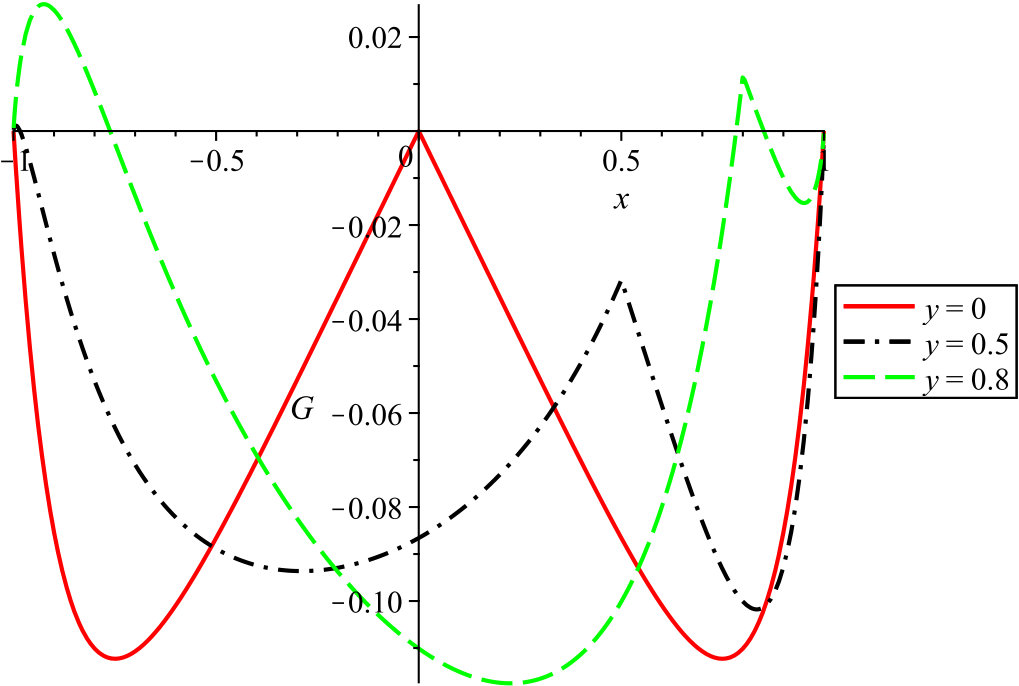 Figure 5
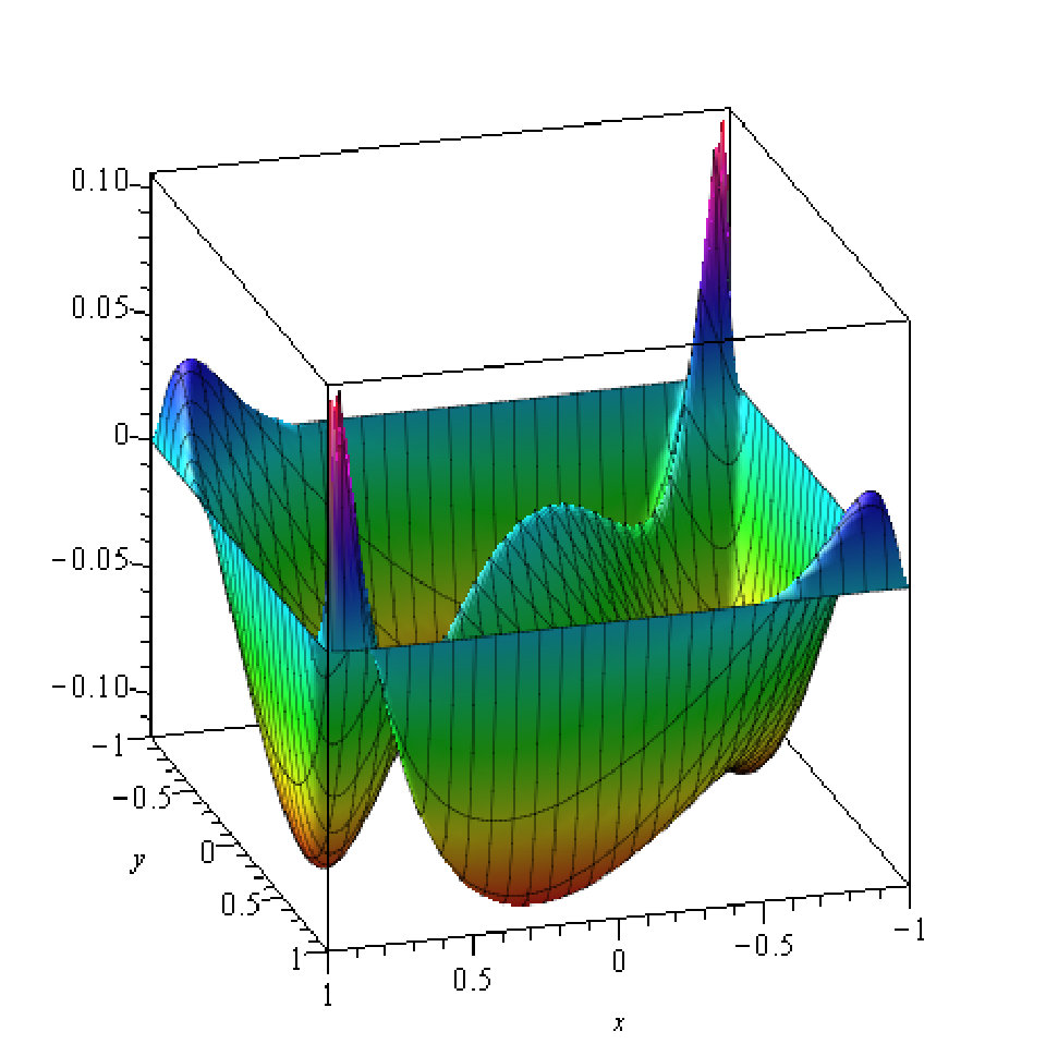 Figure 6
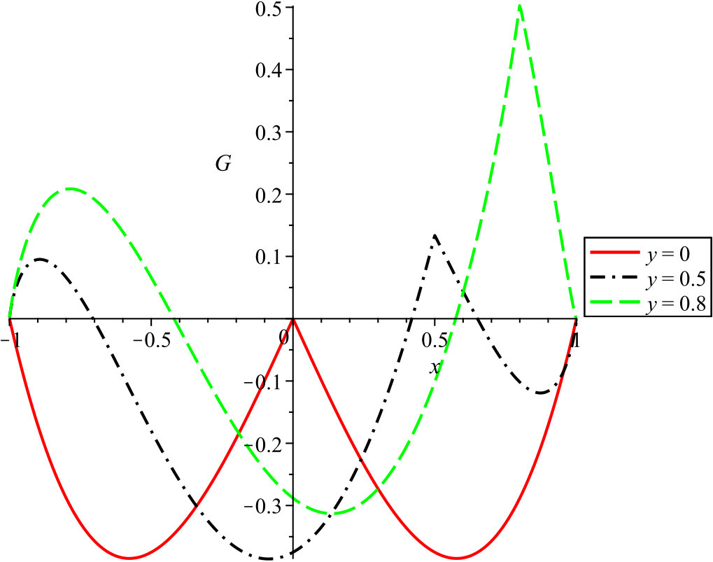 Figure 7
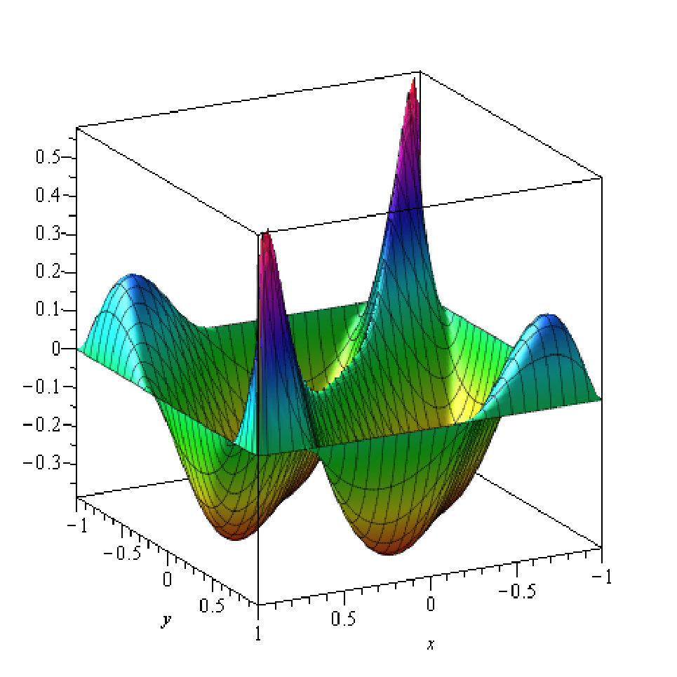 Figure 8
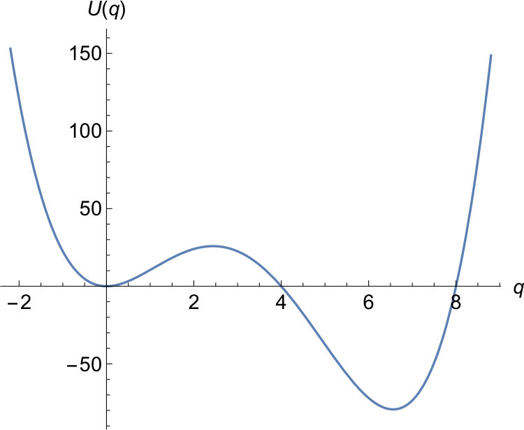 Figure 9
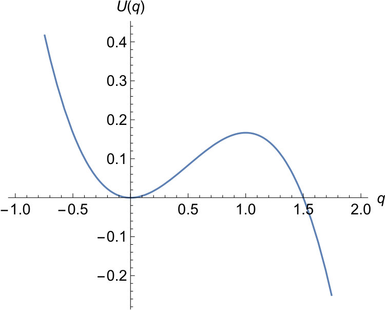 Figure 10
| a11 | ||
| a12 | ||
| b11 | ||
| a21 | ||
| a22 | ||
| a23 | ||
| a24 | ||
| a25 | ||
| b21 | ||
| b22 | ||
| b23 |
| a11 | ||
| a12 | ||
| b11 | ||
| c11 |
Peer Reviews
No public reviews on file for this paper yet. If you reviewed it on a platform where reviews are public (OpenReview, ICLR, NeurIPS, ICML), you can paste yours below so the community can read it here.
Videos
No videos yet. Explain this paper in a talk, walkthrough, or lecture? Add one.
Radiative corrections to false vacuum decay in quantum mechanics
M.A. Bezuglov1,2 A.I. Onishchenko1,2,3
1*Bogoliubov Laboratory of Theoretical Physics, Joint Institute for Nuclear Research, Dubna, Russia,
2Moscow Institute of Physics and Technology (State University), Dolgoprudny, Russia,
3Skobeltsyn Institute of Nuclear Physics, Moscow State University, Moscow, Russia*
Abstract
We consider radiative corrections to false vacuum decay within the framework of quantum mechanics for the general potential of the form , where , and are arbitrary parameters. For this type of potential we provide analytical results for Green function in the background of corresponding bounce solution together with one loop expression for false vacuum decay rate. Next, we discuss the computation of higher order corrections for false vacuum decay rate and provide numerical expressions for two and three loop contributions.
Keywords: false vacuum decays, radiative corrections, quantum mechanics
Contents
1 Introduction
First-order phase transitions driven by scalar fields play an important role in high-energy, astro-particle physics and cosmology. Such first order phase transitions go through the nucleation of new phase bubbles, often around impurities, which subsequently expand. A well known example, which attracted recently a lot of attention, is the possible metastability111For tunneling rates calculations in Standard Model and its extensions see [9, 10, 11, 12, 13, 14, 15, 16, 17] and references therein. of electroweak vacuum at a scale around GeV [1, 2, 3, 4, 5, 6, 7, 8]. Next, first-order phase transitions have a potential of producing stochastic gravitational wave backgrounds [18, 19, 20, 21, 22], which could be further studied experimentally by existing and forthcoming gravitational wave experiments [23]. In addition, first order electroweak phase transition may satisfy Sakharov’s conditions [24] and be responsible for the generation of baryon asymmetry of our Universe, see [25, 26] and references therein. The amount of produced baryon asymmetry crucially depends on the dynamics of phase transition. It should be noted, that in Standard Model the electroweak phase transition is not actually first-order, but a crossover [27, 28, 29, 30]. However, electroweak baryogenesis could survive in its extensions, many of which include extra dynamical scalar fields. The role of impurities catalyzing the mentioned first-order phase transitions may be played by small evaporating black holes or other gravitational inhomogeneities, see [31, 32, 33, 34] and references therein.
The first rigorous description of the mentioned quantum phase transition between different vacuum states appeared in [35, 36, 37, 38]. As is known, the false vacuum decay rate may be related to the imaginary part of ground state energy. However, to calculate the latter one first needs to perform an analytical continuation of the potential so that the false vacuum is stable. This original method was further developed and is known now as potential deformation method, see for review [39, 40, 41, 42, 43, 44]. Recently a more direct way to compute tunneling probabilities using path integrals appeared in [45], see also [44]. In both methods the decay rates are given by path integrals around bounce configurations (solutions of the Euclidean equations of motion used to evaluate path integrals in saddle point approximation) divided by corresponding path integrals around static false vacuum (FV) solutions.
At one loop there is a number of different methods to compute functional determinants arising in evaluation of path integrals. Among them are direct evaluation of spectrum for solvable potentials222See [42] and references therein., heat kernel methods [46, 47, 48, 49], Green function methods [50, 51, 52, 53, 54] and of course famous Gel’fand-Yaglom method [55] and its generalizations [56, 57]. The methods beyond one loop were mostly developed in the study of instantons [58, 59, 60] in quantum mechanics [61, 62, 63, 64, 65], effective Euler-Heisenberg lagrangian [66, 67, 68] and corrections to classical string solutions [69, 70].
The purpose of this paper is to extend the methods of [61, 62, 63, 64, 65] for the computation of higher order radiative corrections to false vacuum decay in quantum mechanics. We organized the paper as follows. In Section 2 we set up our framework and present bounce solutions for the potential of the most general form containing both cubic and quartic interactions. Next, we derive analytical expression for the Green function in the background of found bounce solution. We were able to determine one-loop false vacuum decay rate analytically using Gel’fand-Yaglom method. Beyond one loop we used Feynman diagram technique on the top of false vacuum and bounce solutions to get two and three loop corrections to decay rate. Finally, in Section 3 we come with our conclusion.
2 False vacuum decay in quantum mechanics
The perturbative vacuum obtained by small quantum fluctuations around false (metastable) vacuum will eventually decay. This means that the energy of the ground state has a small imaginary part. The most convenient way to compute ground state energy is to consider small temperature behavior of the thermal partition function
[TABLE]
so that
[TABLE]
The imaginary part of the energy comes from imaginary part of the thermal partition function333See for example [42].
[TABLE]
To compute thermal partition function we will use its path integral representation
[TABLE]
where the Euclidean action is given by
[TABLE]
and the path integral is taken over periodic trajectories, such that
[TABLE]
We will be interested in the general potential of the form
[TABLE]
where , and (, and ) are arbitrary parameters, such that (, , ). The two sets of parameters and are related to each other via
[TABLE]
This particular potential is the most general potential having qubic and quartic interaction terms in addition to the harmonic potential. The typical potentials generally considered in literature arise as its limiting cases. At the same time this particular potential is amenable to analytical treatment similar to the well known case of double well potential. In Fig. 1 we plotted potential for two specific choices of parameters.
As we already mentioned in Introduction the real part of thermal partition function is given by the path integral around false vacuum, while the imaginary part is given by path integral around bounce solution444We refer interested reader for example to [44] for more details. The bounce solution is the solution of classical equation of motion connecting the minima of the potential, which could be easily found using energy conservation for the inverted potential :
[TABLE]
where we have stressed, that we are looking for solution corresponding to classical false vacuum energy. Integrating the above energy conservation condition we get the mentioned bounce solution parameterized by
[TABLE]
Figure 2 contains an example of bounce solution in the limit of small , where and are given by
[TABLE]
[TABLE]
Next, the bounce action is independent of and is given by
[TABLE]
where . The original action (2.5) may be further rewritten in terms of the deviation from the classical configuration, as
[TABLE]
where
[TABLE]
and we have introduced the abbreviation . While making transition to the deviations from bounce solution special care should be taken due to the existence of zero mode of operator . The latter is given by . To integrate over this zero mode we employ Faddeev-Popov-like trick as in [61, 62] and insert into our path integral the unity operator written as555See also [59, 60].
[TABLE]
where
[TABLE]
This way we get
[TABLE]
where is the coefficient in front of our zero mode in the expansion of deviation in terms of eigenfunctions of operator
[TABLE]
We see, that this procedure gives us an extra tadpole vertex coming from integration measure in addition to those we get from lagrangian (LABEL:lagrangian). The presented procedure is known as a transition to collective coordinates. In the case under consideration the only collective coordinate present is given by .
2.1 Green function in the background of bounce solution
The Green function at false vacuum is easy to find and it is given by the solution of corresponding Schrödinger equation:
[TABLE]
or
[TABLE]
where and .
The determination of Green function in the background of bounce solution is more involved. As we have already seen in previous section the corresponding inverse operator has zero mode. The inversion of the latter is consistently defined only on the subspace of functions orthogonal to this zero mode (Fredholm alternative). More concretely, the Green function we will be looking for is defined as666The normalization of wave functions to unity is assumed.
[TABLE]
where and the summation goes over all modes except zero one. It is easy to check that the equation satisfied by this Green function is given by
[TABLE]
or
[TABLE]
where and
[TABLE]
First solution of the homogeneous equation is given by the zero mode of operator we found in previous section:
[TABLE]
The second solution may be found using the so-called reduction of order method. First, from Abel’s differential equation identity we get an equation for Wronskian of homogeneous solutions :
[TABLE]
Integrating the latter together with subsequent first order differential equation (obtained from known expressions for Wronskian and first homogeneous solution) for we get
[TABLE]
The particular solution of nonhomogeneous solution is then found by the variation of constants and is given by
[TABLE]
where
[TABLE]
The integrals in the above expression could be evaluated in terms of polylogarithms. However, the expressions we get are quite lengthy and we put them in mathematica file accompanying this article. Here, we will present analytical expressions only for two particular cases. In the limit777One should take a limit and not just set to zero. we get
[TABLE]
and in the case the particular solution takes the form:
[TABLE]
where
[TABLE]
The Green function in the background of bounce solution is then given by
[TABLE]
with and are some arbitrary functions of variable . The latter are determined from the conditions:
is finite for (); 2. 2.
is continuous at (); 3. 3.
is orthogonal to the zero mode (2.27) (we accounted for the Jacobian of transition from to , ):
[TABLE]
Using the first two conditions together with the fact that Green function is symmetric with respect to the exchange of variables we were able to determine Green function analytically up to one unknown constant. The latter could be found using third condition numerically. The resulting expression for Green function is too lengthy and could be found in accompanying mathematica file. In the limit the analytical expression is quite short and the corresponding Green function is given by ( or )
[TABLE]
where
[TABLE]
[TABLE]
and
[TABLE]
Finally, figures 3 and 4 contain plots of Green functions in the background of bounce solution for two sets of parameters and .
2.2 One loop expression
At one loop the real and imaginary parts of our thermal partition function are given by888See for example [42, 44]. ( is the partition function evaluated by the expansion at false vacuum ):
[TABLE]
so, that for imaginary part of energy we get
[TABLE]
The easy way to derive an expression for the ratio of functional determinants is to use the formalism of Gel’fand and Yaglom [55], see also [42, 49]. Within the latter, given a Schödinger operator defined on the interval with eigenfunctions satisfying Dirichlet999In the zero temperature case considered here it is enough to consider Dirichlet boundary conditions. boundary conditions
[TABLE]
its determinant is found as a solution of the auxiliary problem
[TABLE]
so, that
[TABLE]
In general the above determinants diverge, so one generally considers their ratio
[TABLE]
This result could be straightforwardly obtained using contour integration technique of Kirsten and McKane [56, 57]. Indeed, writing the eigenvalue problem as
[TABLE]
and noting that if satisfies the Dirichlet boundary conditions on both sides of the interval, i.e. if also
[TABLE]
then becomes the eigenvalue of and the sum of chosen powers of all eigenvalues of the latter could be conveniently represented by the following contour integral
[TABLE]
where the contour runs counterclockwise and we used the fact, that in the vicinity of eigenvalue
[TABLE]
The logarithmic derivative converges101010At large the potential in Scrödinger operator could be neglected and we have . as and the integration contour could be deformed as we wish. Deforming the latter to imaginary axis we get
[TABLE]
Recalling now that the operator determinants could be expressed as exponentials of the introduced zeta functions derivatives at zero, the determinant ratio is given by
[TABLE]
The presented derivation is valid if the considered operators do not contain zero modes. In our case does actually have a zero mode due to time translation invariance and the above contour deformation is ill defined as is zero at . To overcome this difficulty we need to know the behavior of for small to eliminate the pole in integrand. Integrating by parts the left hand side of
[TABLE]
gives
[TABLE]
Using the boundary conditions for and we get111111We dropped the as we are dealing with real solutions only.
[TABLE]
It is easy to see that due to the orthogonality of eigenfunctions vanishes for all values of except at , where it remains non-zero. A function which behaves as for large but is non-zero for is given by , so the contour integral associated with the determinant of is given by
[TABLE]
where the zero mode from was omitted. The second integral on the right hand side is easily taken by a residue at simple pole and we get
[TABLE]
The expression for the corresponding determinant ratio is then given by
[TABLE]
where denotes the determinant with zero eigenvalue omitted. The expression for function in the case of functional determinant around bounce solution could be easily found using the methods presented in previous section and is given by
[TABLE]
Here, we assumed that the parameter of the bounce solution was chosen, so that . This result could be easily generalized for more complicated boundary conditions both with and without zero modes [56, 57]. Finally, in our particular case we get
[TABLE]
so that the imaginary part of energy is given by
[TABLE]
We have checked that the same expression is reproduced using formula presented in [50, 51]. Moreover, it could be also obtained using slight modification of the derivation presented in [42] for the case of . The above determinant ratio in this case is given by
[TABLE]
where is the zero of potential and turning point for the bounce solution. In our case . The corresponding imaginary part of energy is then found with
[TABLE]
2.3 Non-gaussian effects
To calculate higher order corrections we are following [61, 62, 63, 64, 65] and use Feynman diagram technique on top of false vacuum and bounce solution. The first is used to calculate higher order contributions to real part of thermal partition function, while the latter for higher order radiative corrections to its imaginary part. The corresponding Feynman rules are easy to derive and they are given by
[TABLE]
Note, that Feynman diagrams on top of bounce solution may contain single tadpole vertex coming from the Jacobian of transition to collective coordinate (2.19). Such diagrams appear only for the expansion on top of bounce solution and are absent in the case of false vacuum. The Green functions for the cases of false vacuum and bounce solution were given in previous subsection. Figures 5, 6 and 7 contain two and tree loop diagrams containing only cubic vertexes, tadpole vertex and extra quartic vertexes correspondingly. The diagram expressions with account for symmetry factors are constructed as it is usually done in quantum field theory. For example, the expression for Feynman diagram (see Fig. 6) is given by:
[TABLE]
where is the Jacobian of transition from to variables.
Diagrams without tadpole vertexes are present both in corrections to real and imaginary parts of thermal partition function. As the imaginary part of energy we are interested in is defined by their ratio it is convenient to combine these contributions, so that for example the difference of corresponding diagrams for bounce and false vacuum solutions is given by:
[TABLE]
To calculate two and three loop corrections to the false vacuum decay rate for arbitrary values of parameters one may use the mathematica notebook accompanying this article, where required numerical integrations are performed with the help of CUBA library [71]. Here we will present results only for two particular cases used throughout this paper. In the limit the imaginary part of energy up to three-loop accuracy is given by
[TABLE]
where in this case and are two loop and - three loop contributions (see Tables 1 and 2):
[TABLE]
with
[TABLE]
and
[TABLE]
In the case the corresponding corrections are given by (see Tables 3 and 4 for the contributions of individual diagrams):
[TABLE]
where
[TABLE]
and
[TABLE]
We see that in the case with the higher order corrections are small and could be safety neglected. On the other hand in the limit the radiative corrections could be sizeable if and thus should be taken into account.
3 Conclusion
In this paper we considered the calculation of false vacuum decay rate for the case of arbitrary potential containing both cubic and quartic interactions in the framework of quantum mechanics. We obtained analytical expressions both for Green functions in the background of bounce solutions as well as for one-loop false vacuum decay rate. Besides, we provided numerical results for two and three-loop contributions to the decay rate together with a mathematica notebook, which could be used to evaluate two and three loop radiative corrections for arbitrary values of cubic and quartic couplings. The presented techniques could be further generalized to the case of quantum field theory, which will be our next step.
Acknowledgements
The authors would like to thank A.V. Bednyakov, A.E. Bolshov, M.Yu. Kalmykov, D.I. Kazakov, D.I. Melikhov, V.N. Velizhanin, O.L. Veretin and A.F. Pikelner for interesting and stimulating discussions. This work was supported by RFBR grants # 17-02-00872, # 16-02-00943 and contract # 02.A03.21.0003 from 27.08.2013 with Russian Ministry of Science and Education.
The reference list from the paper itself. Each links out to its DOI / PubMed record.
- 1[1] J. Elias-Miro, J. R. Espinosa, G. F. Giudice, G. Isidori, A. Riotto and A. Strumia, Higgs mass implications on the stability of the electroweak vacuum , Phys. Lett. B 709 , 222 (2012) [ar Xiv:1112.3022 [hep-ph]].
- 2[2] G. Degrassi, S. Di Vita, J. Elias-Miro, J. R. Espinosa, G. F. Giudice, G. Isidori and A. Strumia, Higgs mass and vacuum stability in the Standard Model at NNLO , JHEP 1208 , 098 (2012) [ar Xiv:1205.6497 [hep-ph]].
- 3[3] F. Bezrukov, M. Y. Kalmykov, B. A. Kniehl and M. Shaposhnikov, Higgs Boson Mass and New Physics , JHEP 1210 , 140 (2012) [ar Xiv:1205.2893 [hep-ph]].
- 4[4] S. Alekhin, A. Djouadi and S. Moch, The top quark and Higgs boson masses and the stability of the electroweak vacuum , Phys. Lett. B 716 , 214 (2012) [ar Xiv:1207.0980 [hep-ph]].
- 5[5] I. Masina, Higgs boson and top quark masses as tests of electroweak vacuum stability , Phys. Rev. D 87 , no. 5, 053001 (2013) [ar Xiv:1209.0393 [hep-ph]].
- 6[6] D. Buttazzo, G. Degrassi, P. P. Giardino, G. F. Giudice, F. Sala, A. Salvio and A. Strumia, Investigating the near-criticality of the Higgs boson , JHEP 1312 , 089 (2013) [ar Xiv:1307.3536 [hep-ph]].
- 7[7] J. R. Espinosa, G. F. Giudice, E. Morgante, A. Riotto, L. Senatore, A. Strumia and N. Tetradis, The cosmological Higgstory of the vacuum instability , JHEP 1509 , 174 (2015) [ar Xiv:1505.04825 [hep-ph]].
- 8[8] A. V. Bednyakov, B. A. Kniehl, A. F. Pikelner and O. L. Veretin, Stability of the Electroweak Vacuum: Gauge Independence and Advanced Precision , Phys. Rev. Lett. 115 , no. 20, 201802 (2015) [ar Xiv:1507.08833 [hep-ph]].