A nonlinear method for imaging with acoustic waves via reduced order model backprojection
Vladimir Druskin, Alexander V. Mamonov, Mikhail Zaslavsky

TL;DR
This paper presents a nonlinear, data-driven imaging method for acoustic waves that improves resolution and reduces artifacts by using reduced order models and a novel orthogonalization process based on measured data.
Contribution
It introduces a nonlinear imaging approach using reduced order models derived from data, enhancing resolution and artifact suppression over traditional linear methods.
Findings
Improves imaging resolution compared to RTM.
Effectively removes multiple reflection artifacts.
Achieves accurate imaging with imperfect velocity models.
Abstract
We introduce a novel nonlinear imaging method for the acoustic wave equation based on data-driven model order reduction. The objective is to image the discontinuities of the acoustic velocity, a coefficient of the scalar wave equation from the discretely sampled time domain data measured at an array of transducers that can act as both sources and receivers. We treat the wave equation along with transducer functionals as a dynamical system. A reduced order model (ROM) for the propagator of such system can be computed so that it interpolates exactly the measured time domain data. The resulting ROM is an orthogonal projection of the propagator on the subspace of the snapshots of solutions of the acoustic wave equation. While the wavefield snapshots are unknown, the projection ROM can be computed entirely from the measured data, thus we refer to such ROM as data-driven. The image is…
Click any figure to enlarge with its caption.
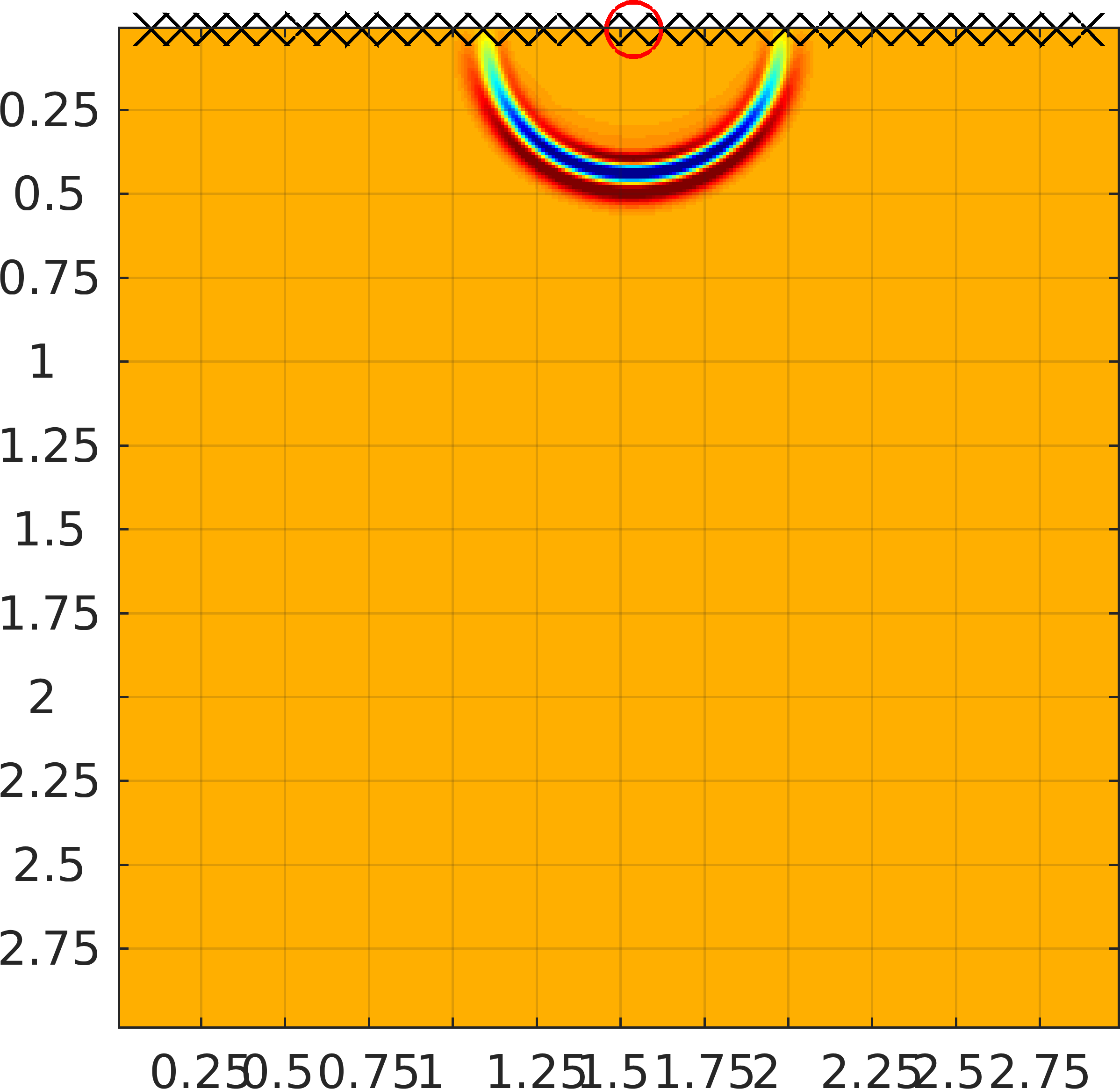 Figure 1
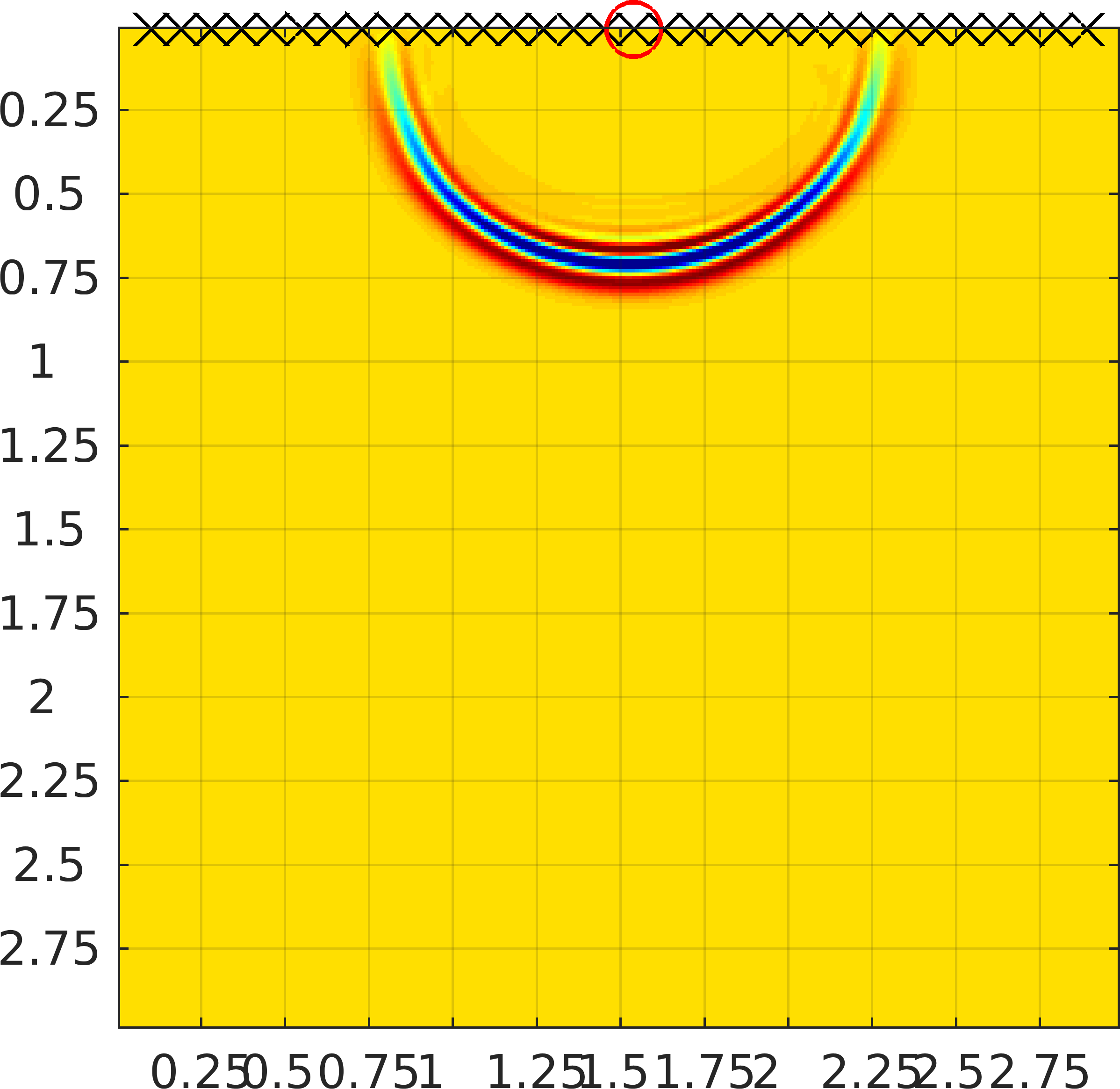 Figure 2
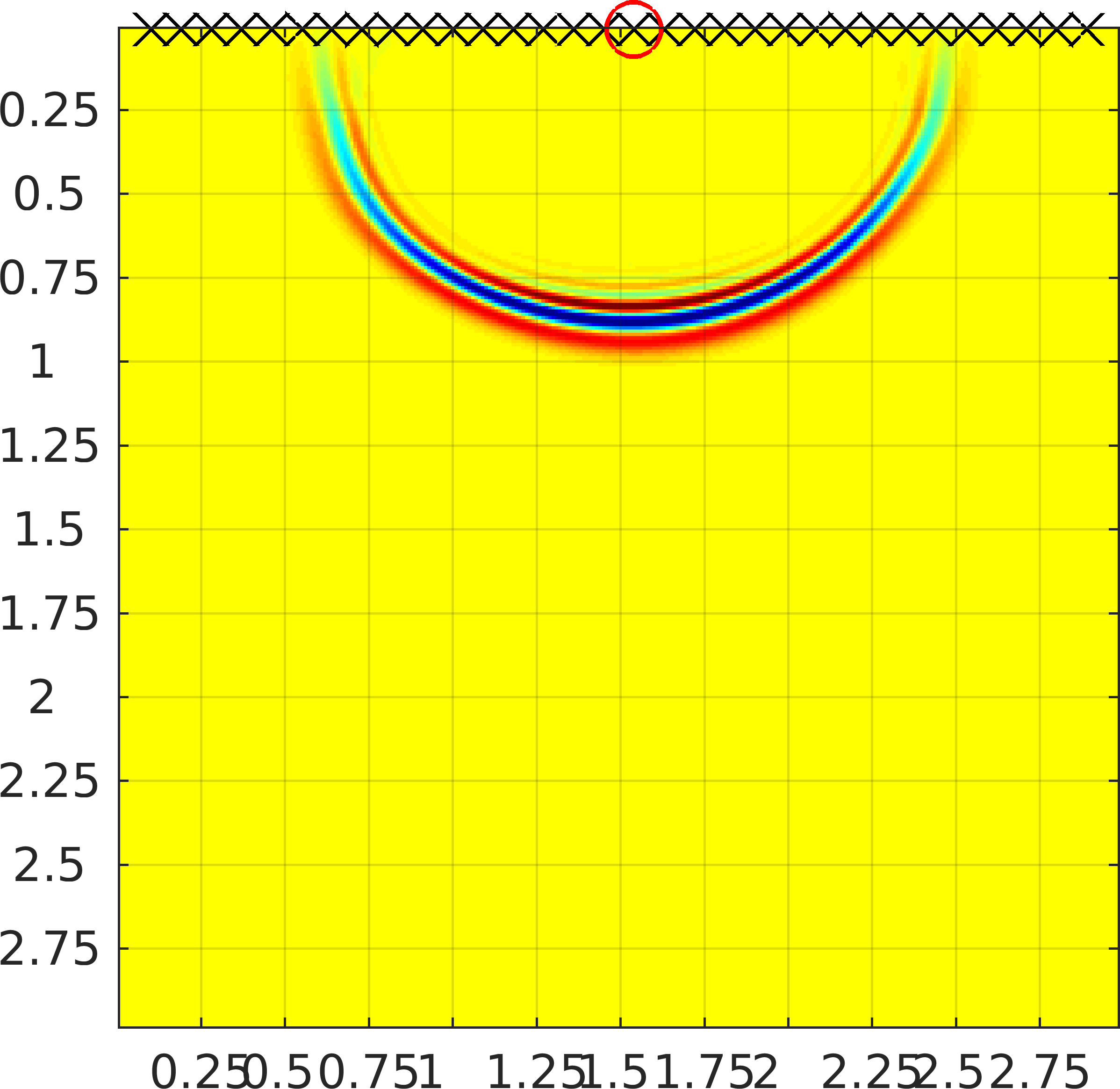 Figure 3
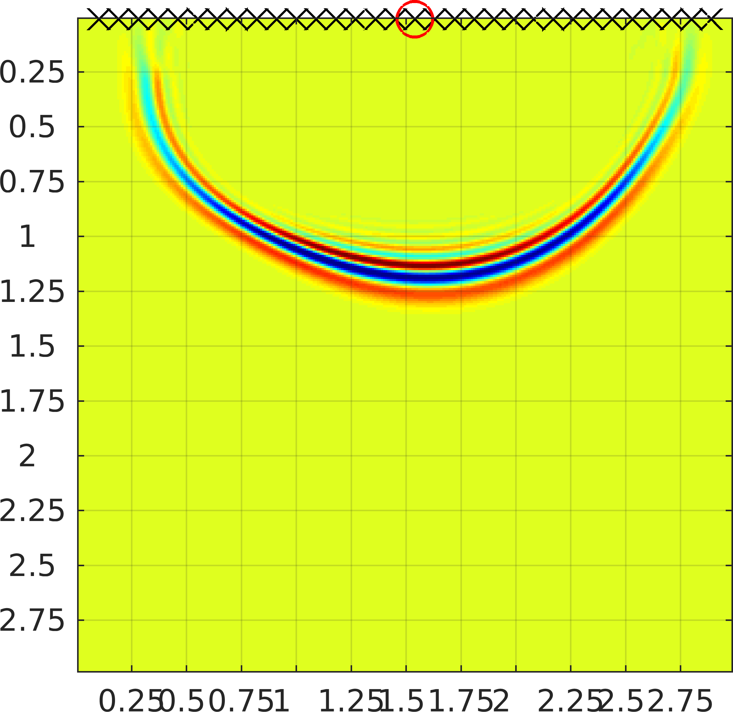 Figure 4
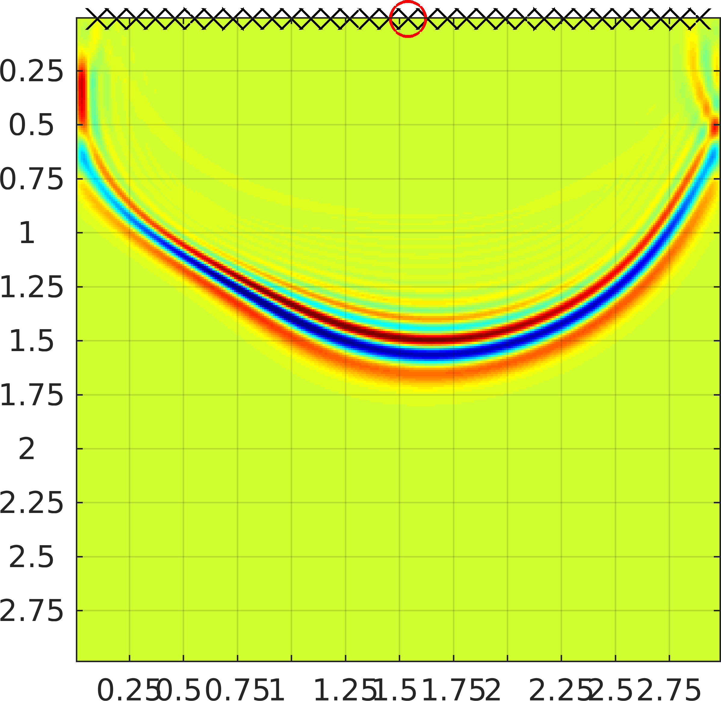 Figure 5
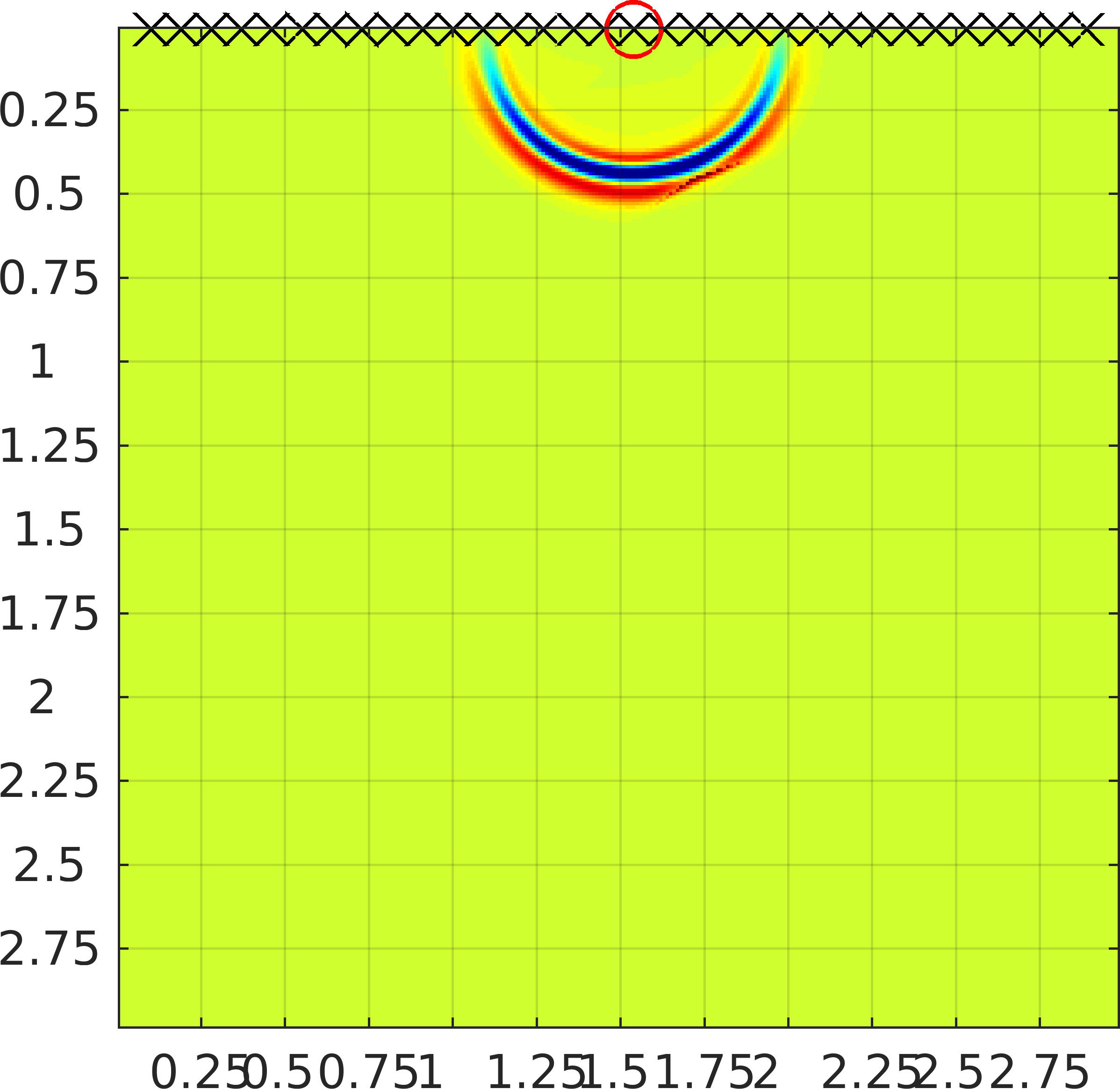 Figure 6
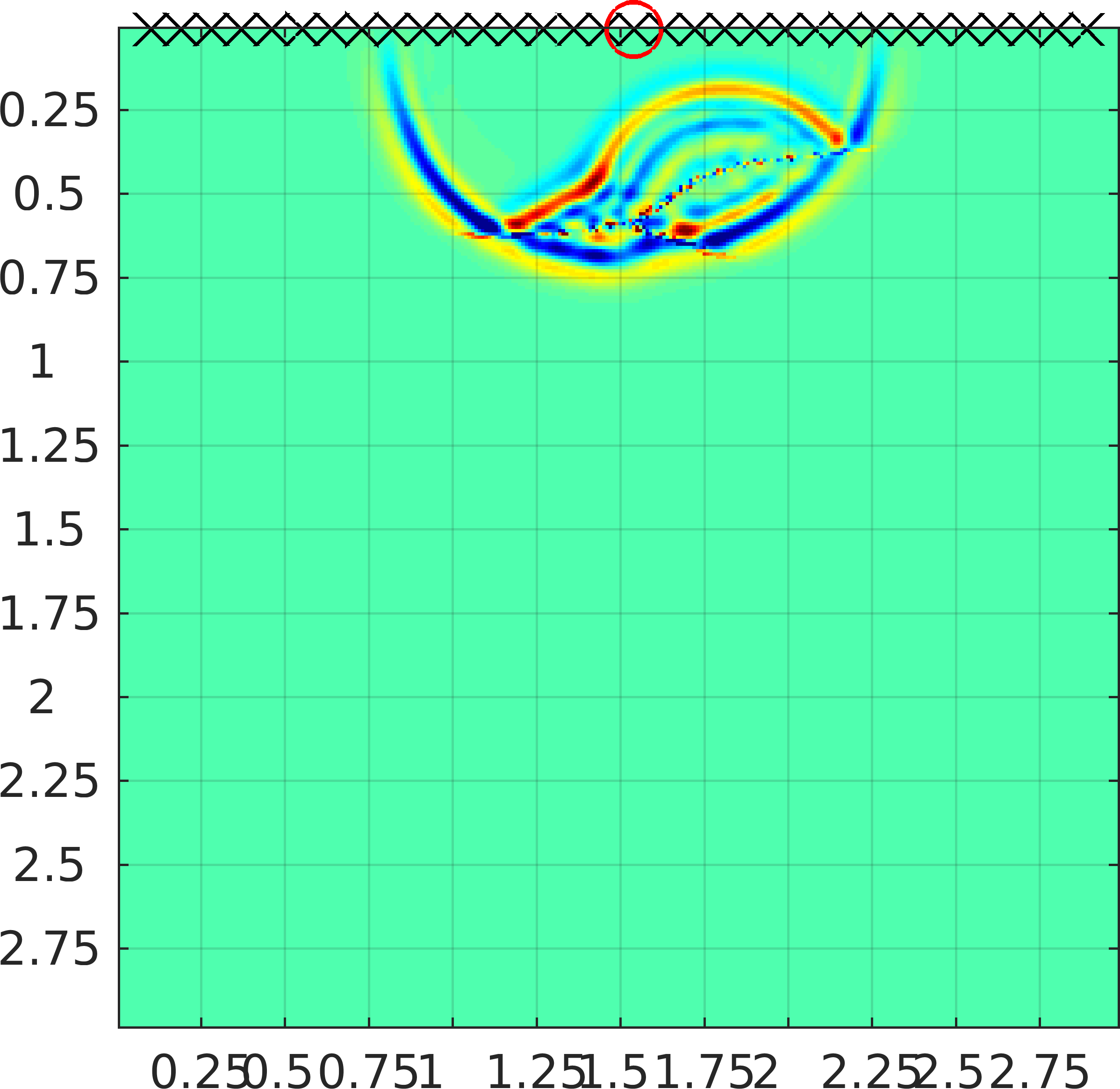 Figure 7
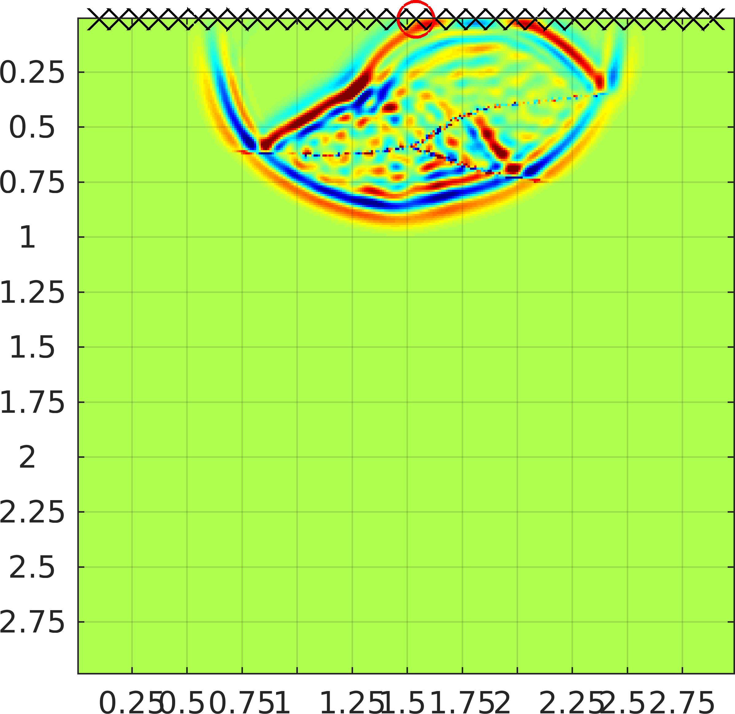 Figure 8
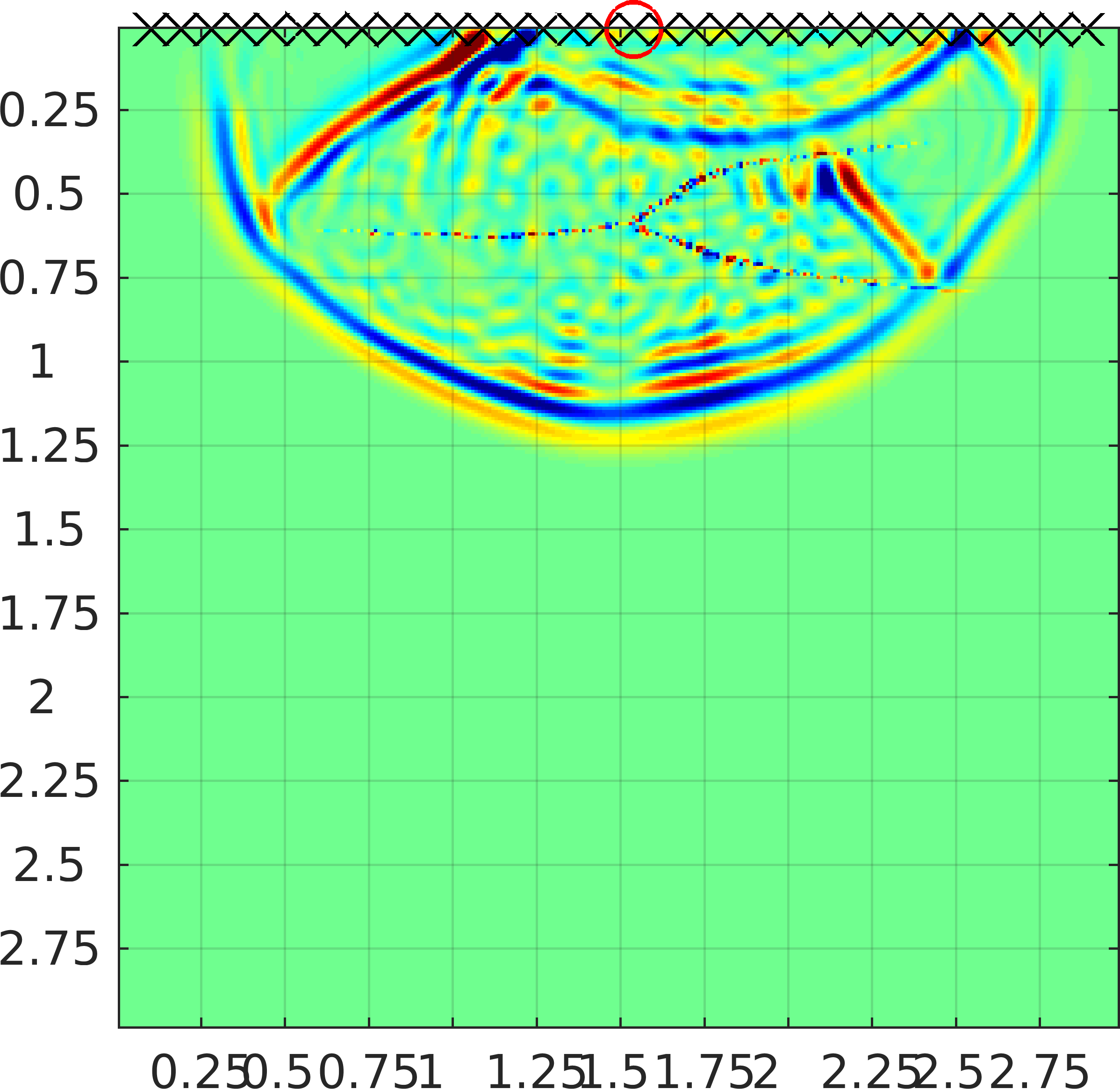 Figure 9
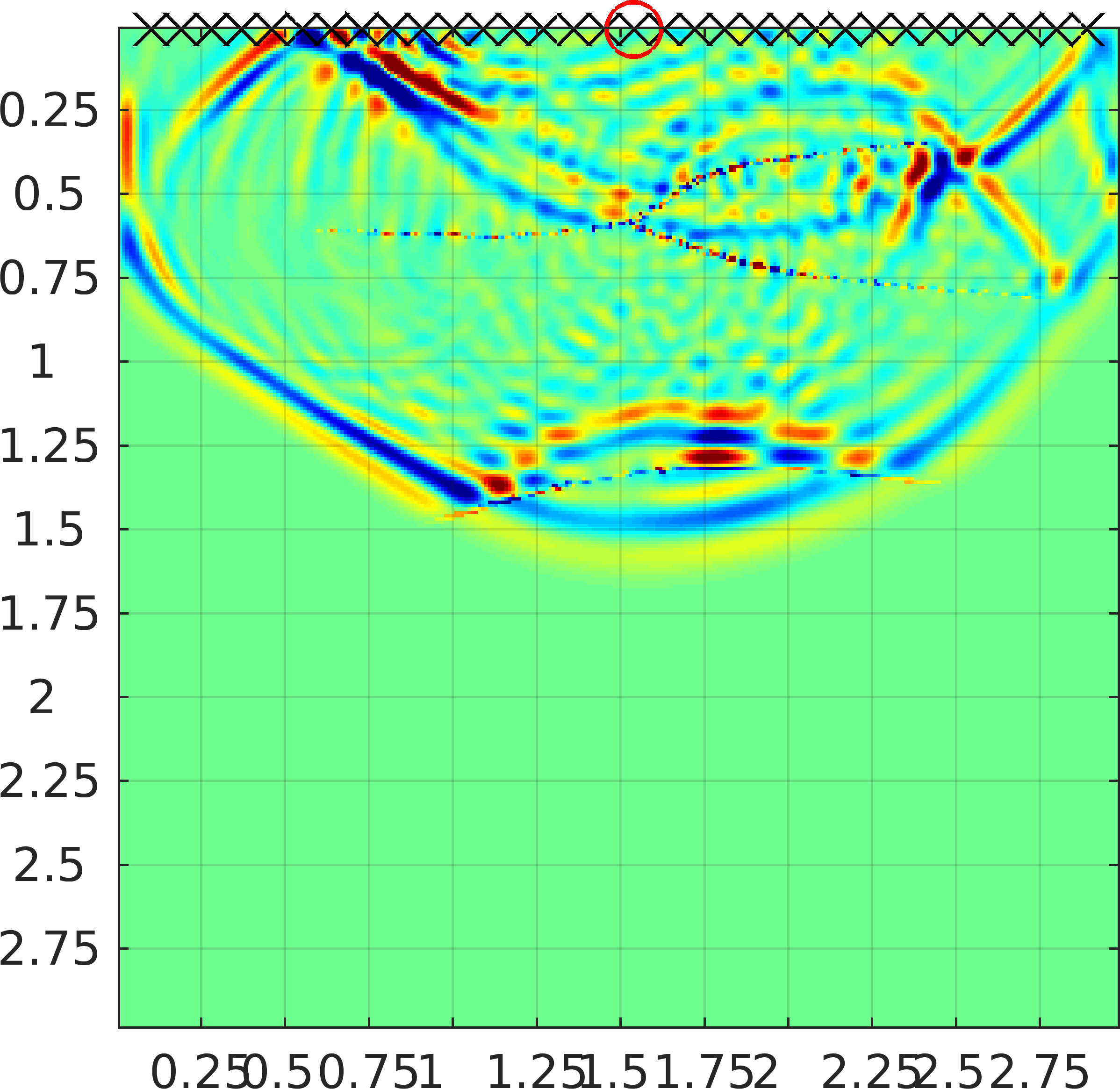 Figure 10
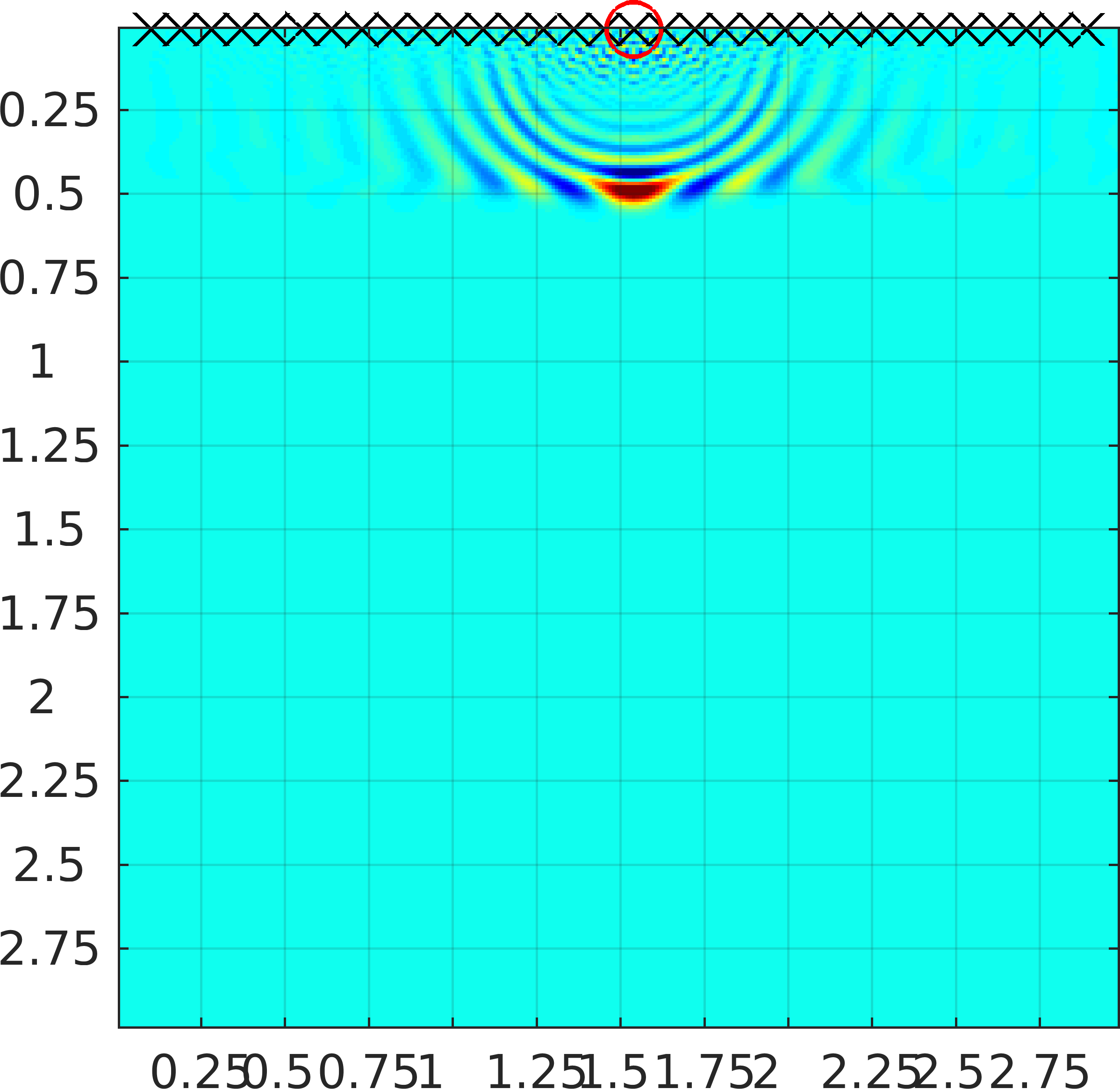 Figure 11
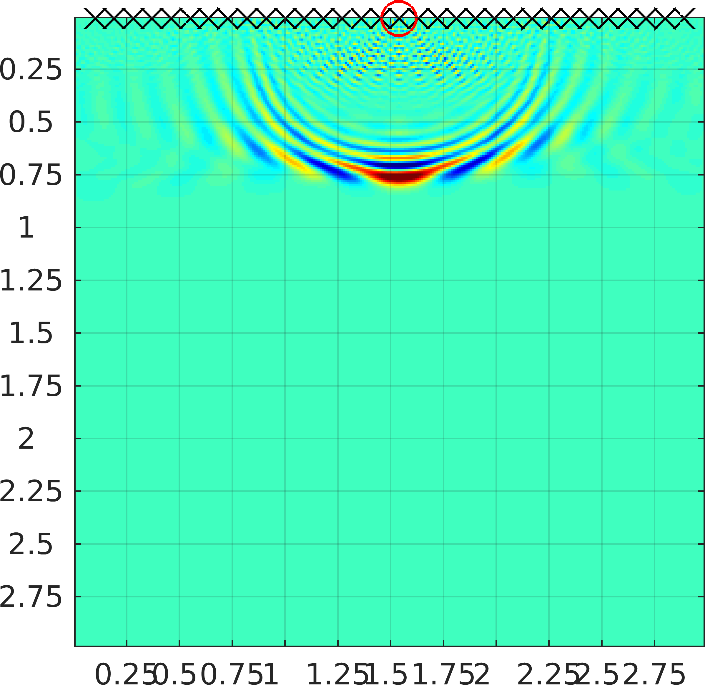 Figure 12
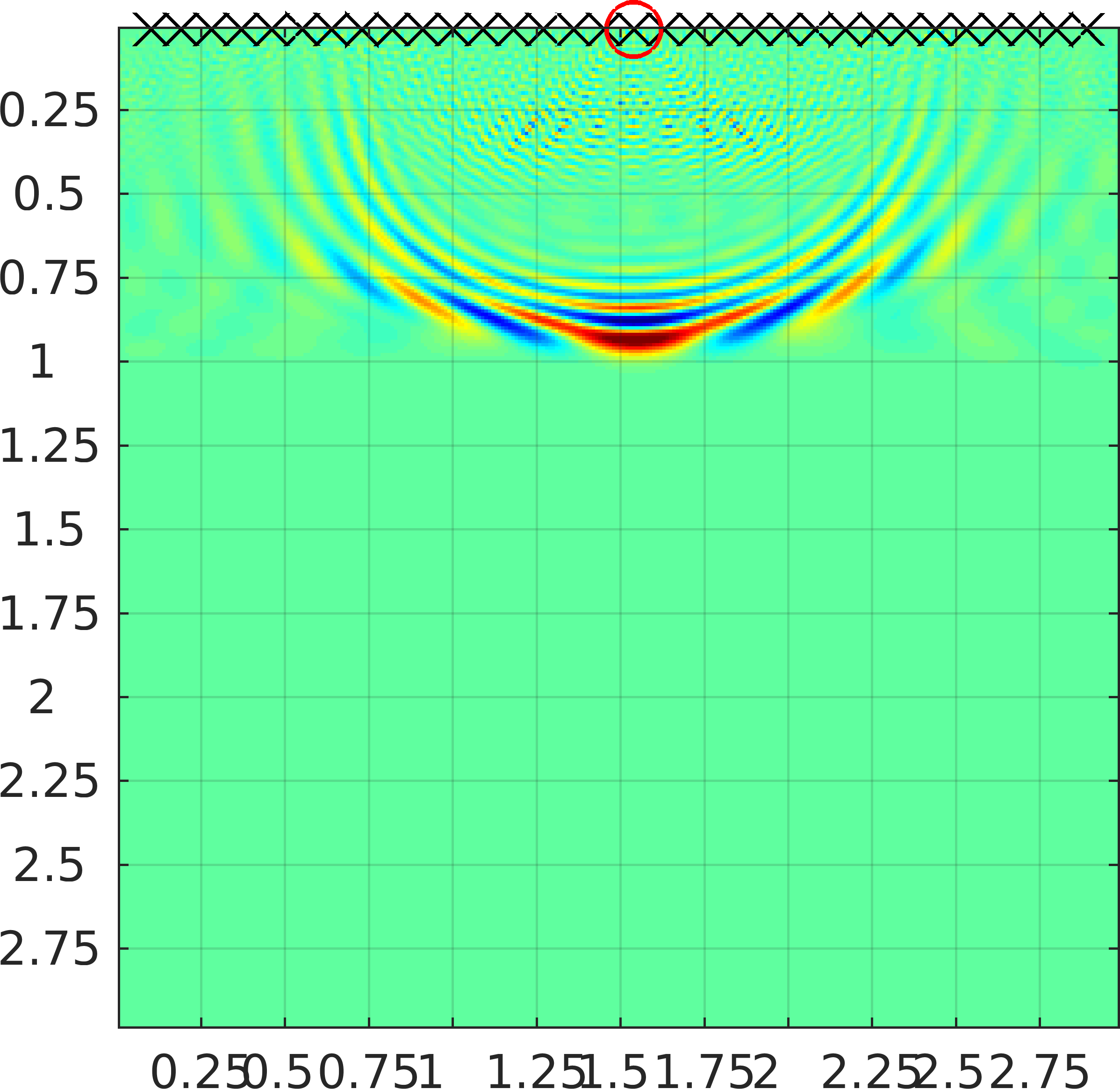 Figure 13
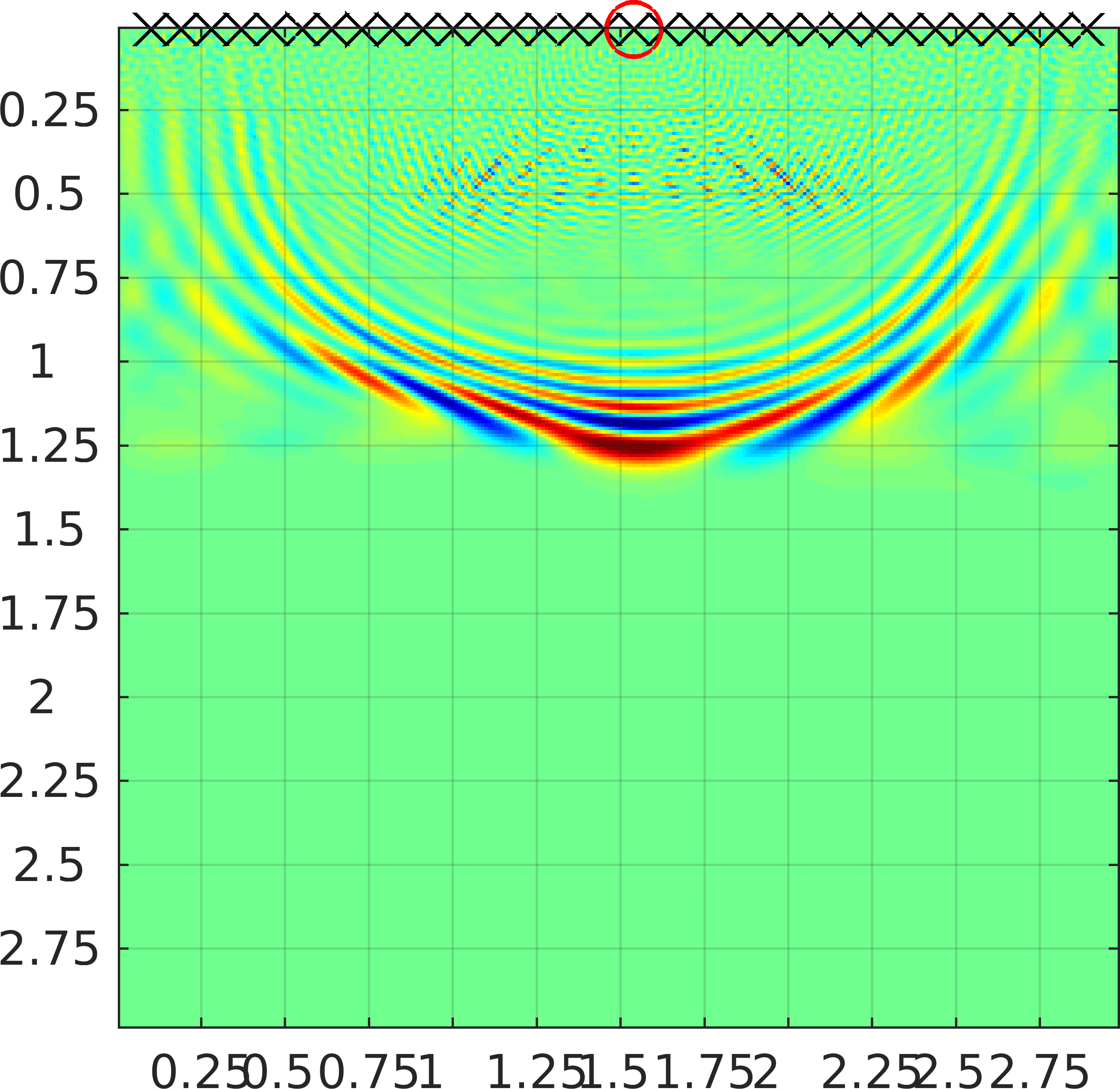 Figure 14
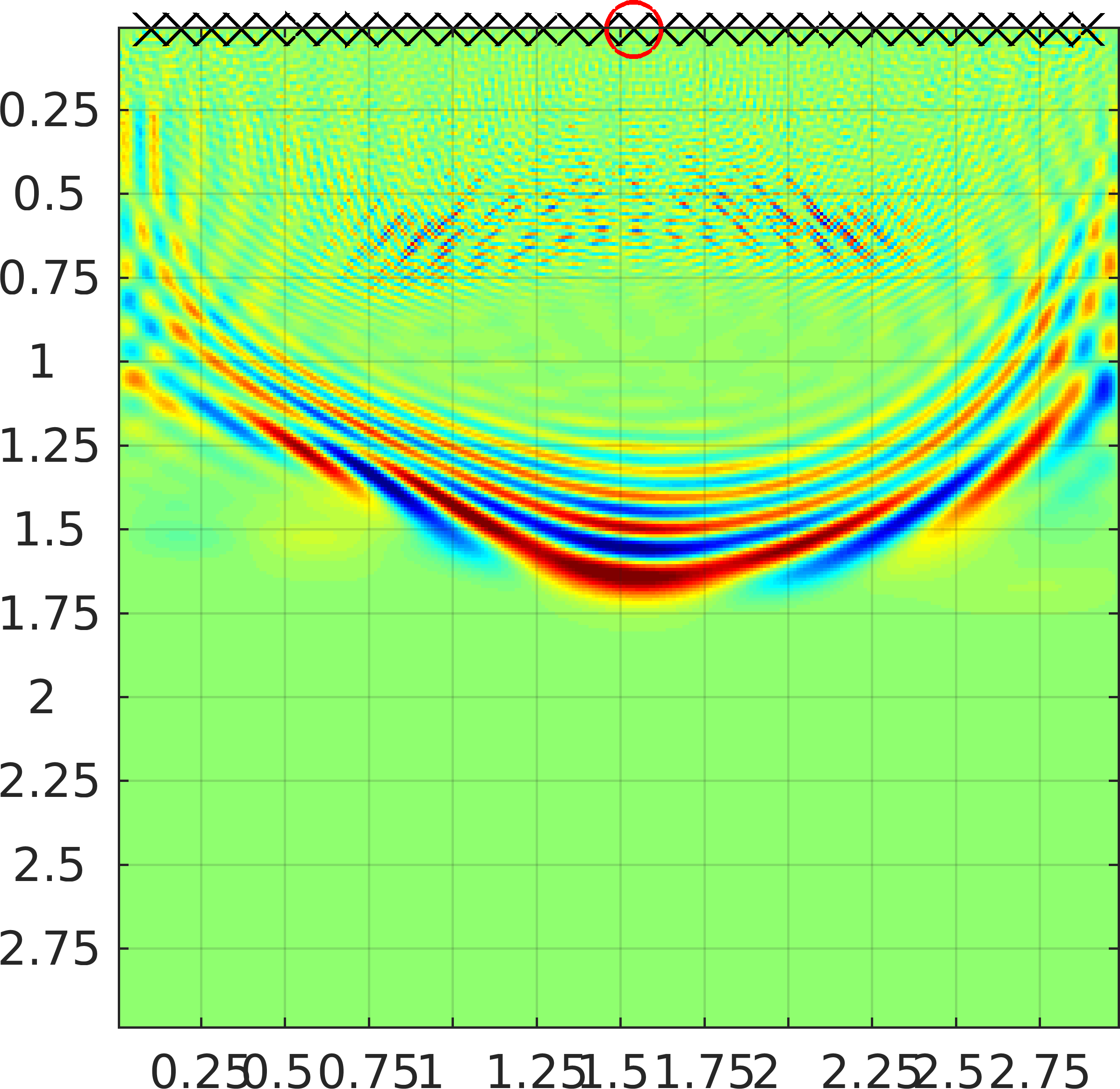 Figure 15
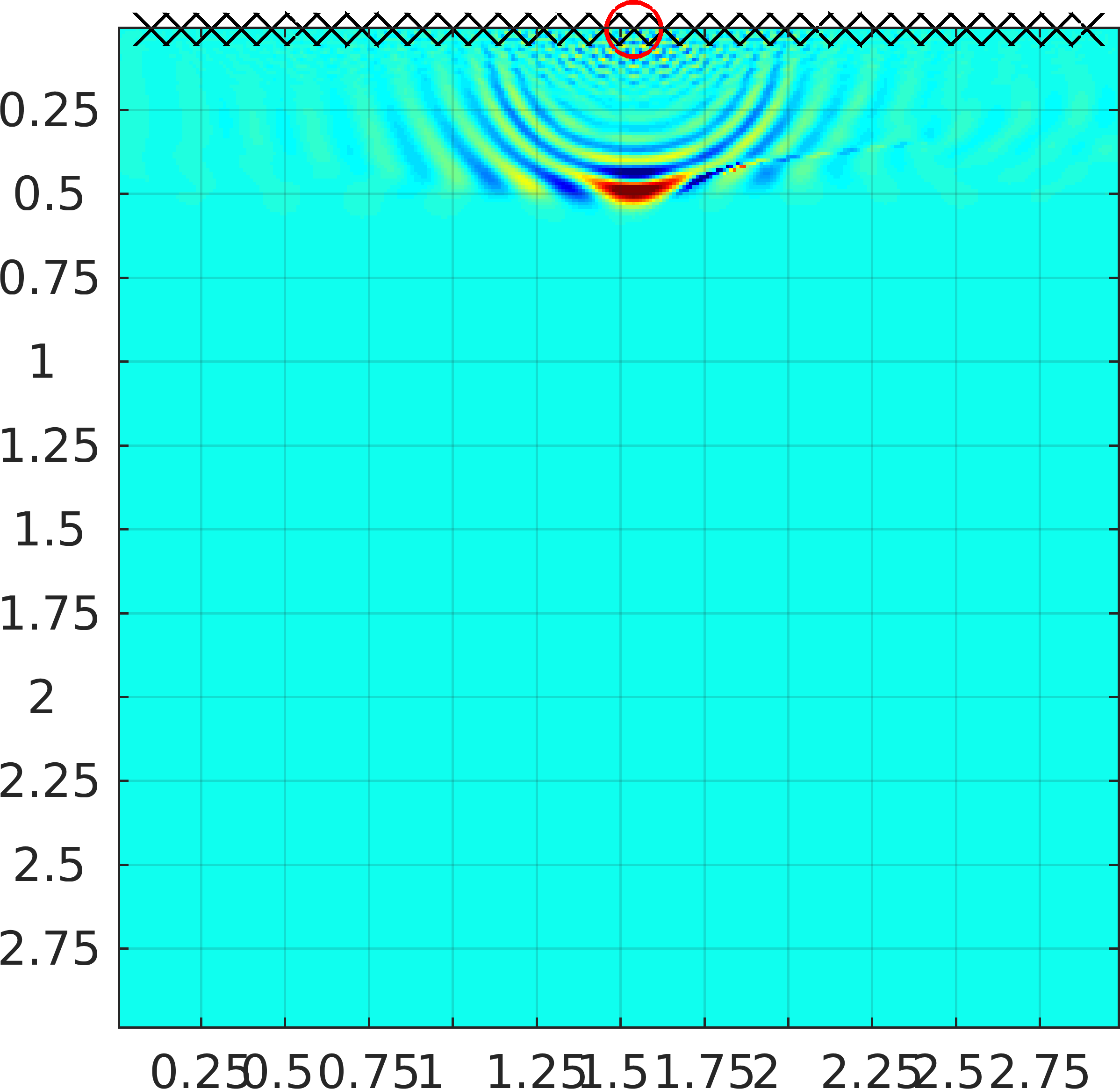 Figure 16
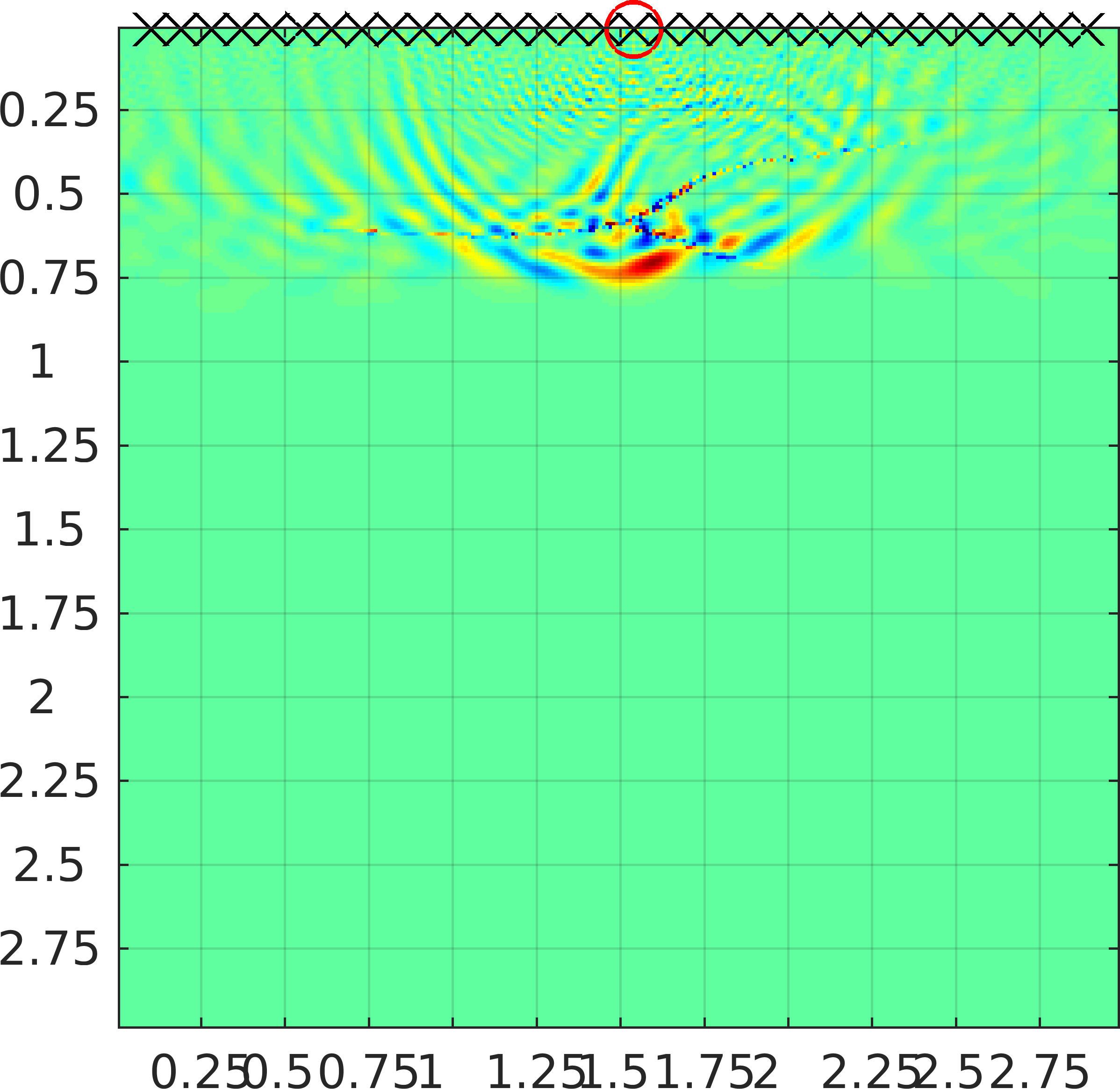 Figure 17
 Figure 18
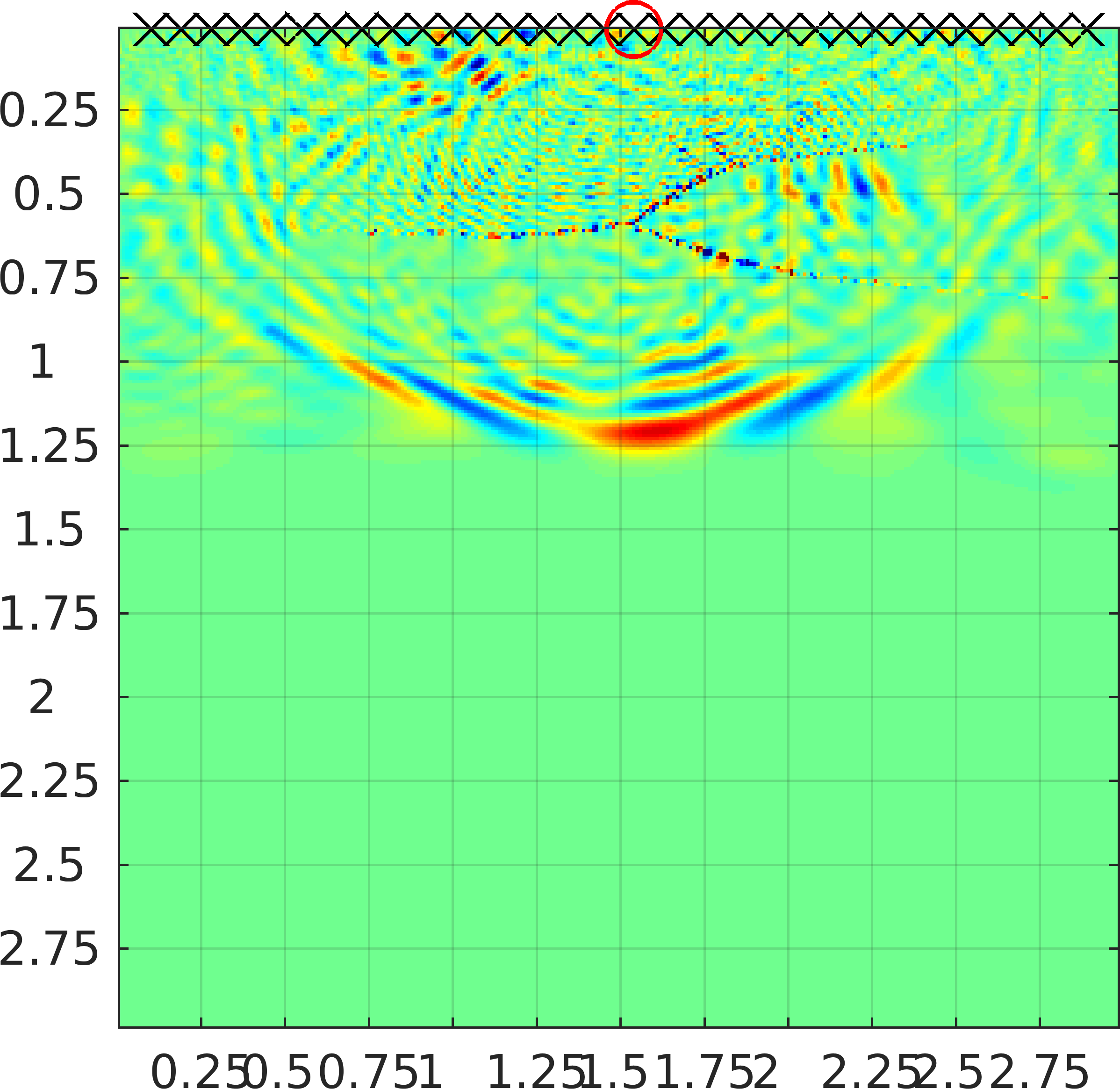 Figure 19
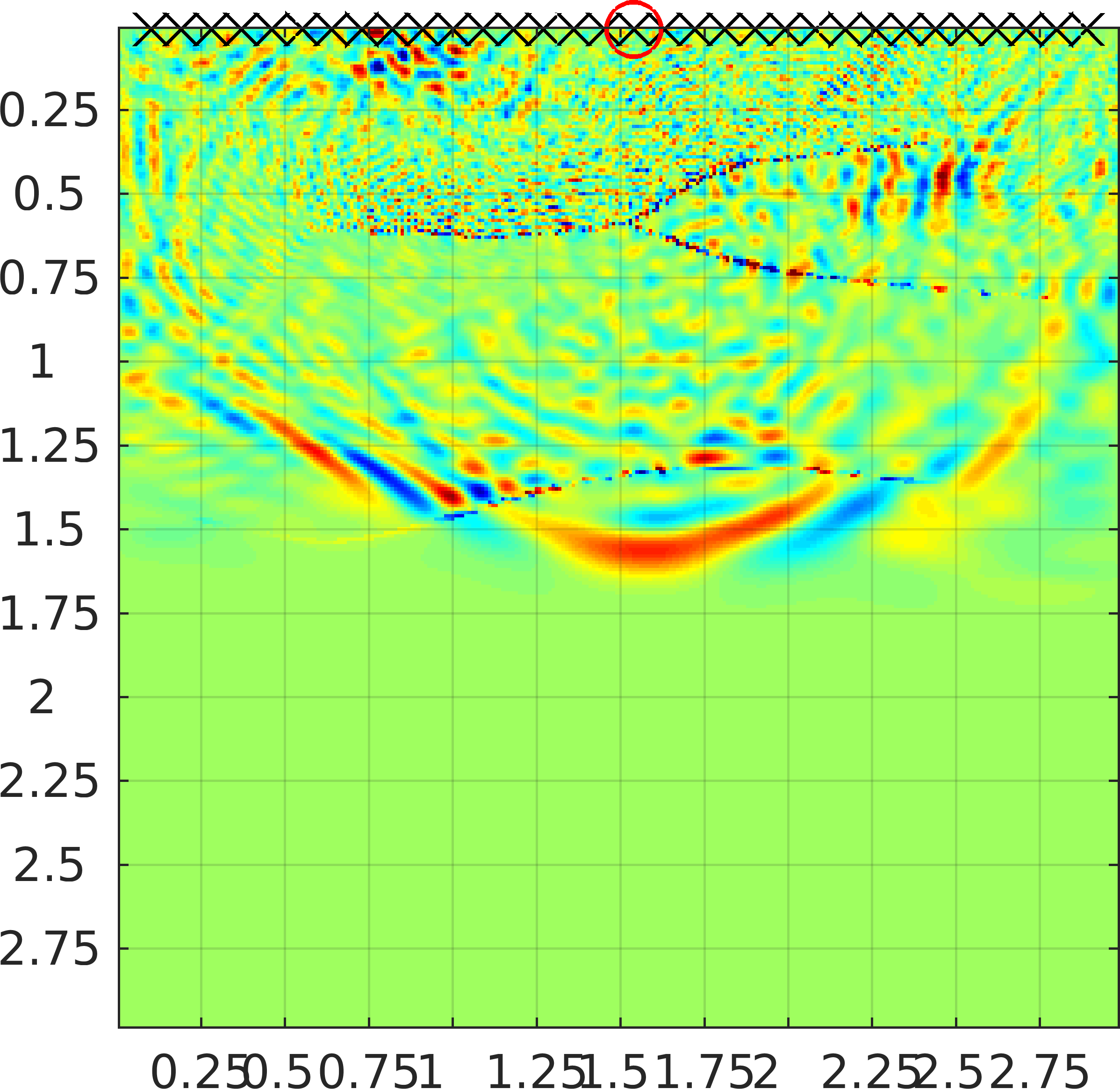 Figure 20
 Figure 21
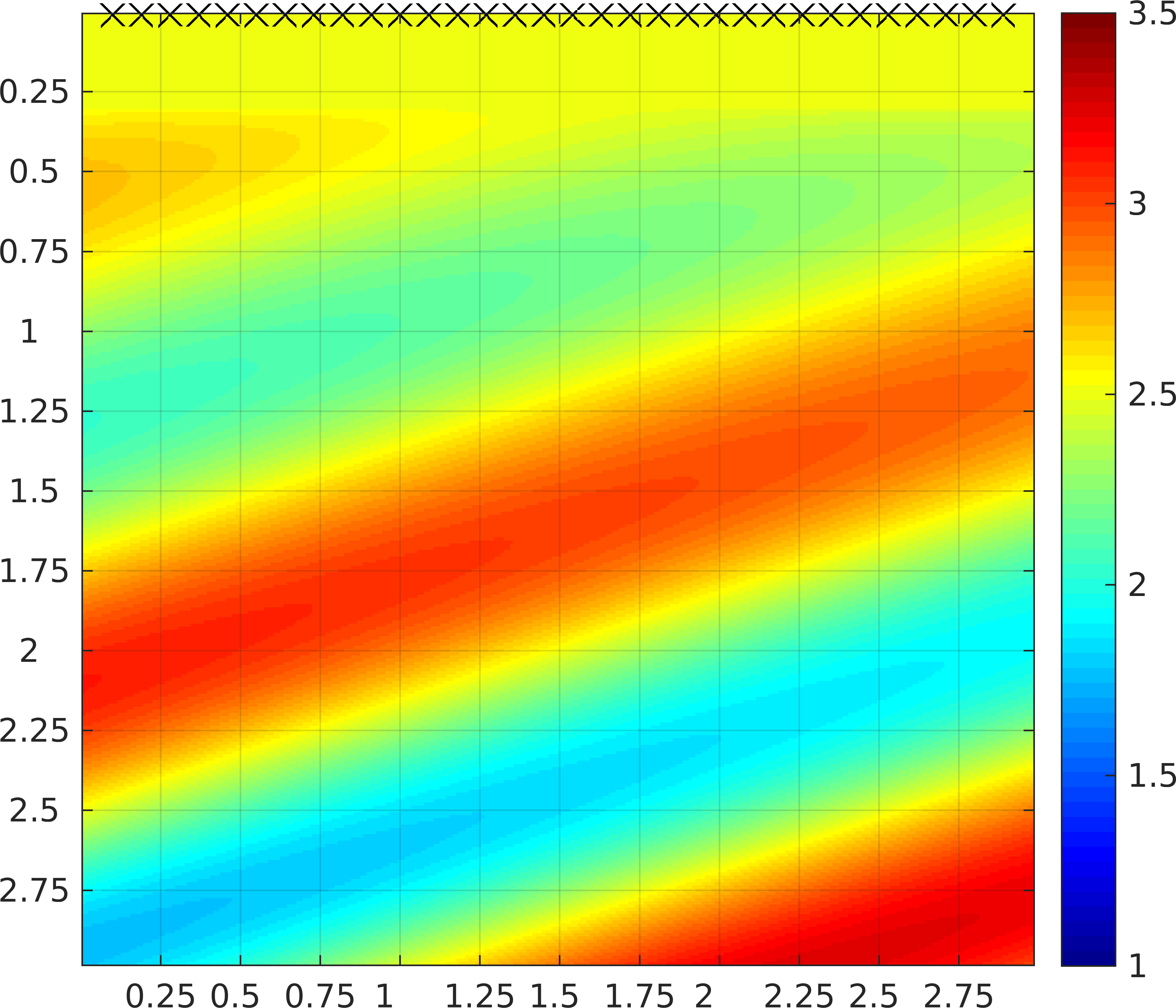 Figure 22
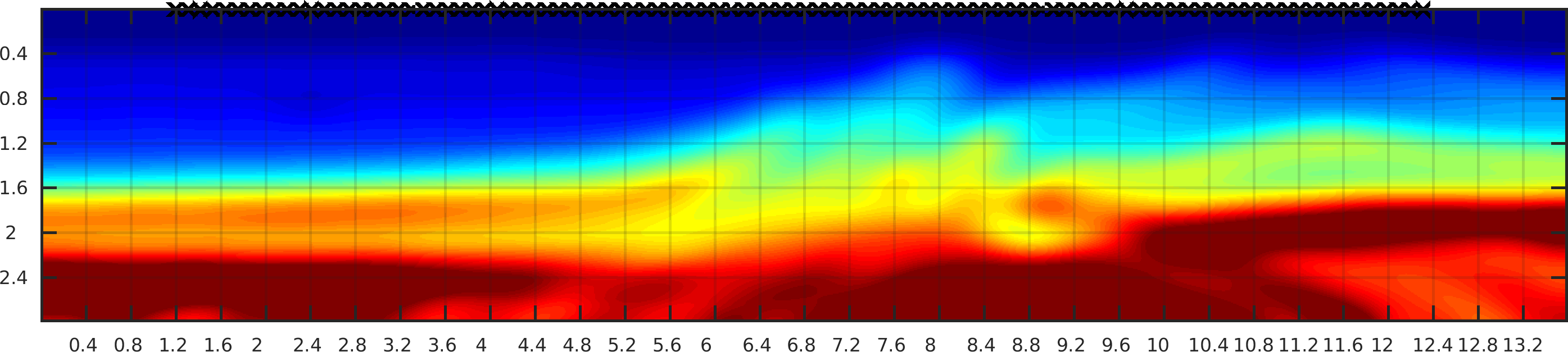 Figure 23
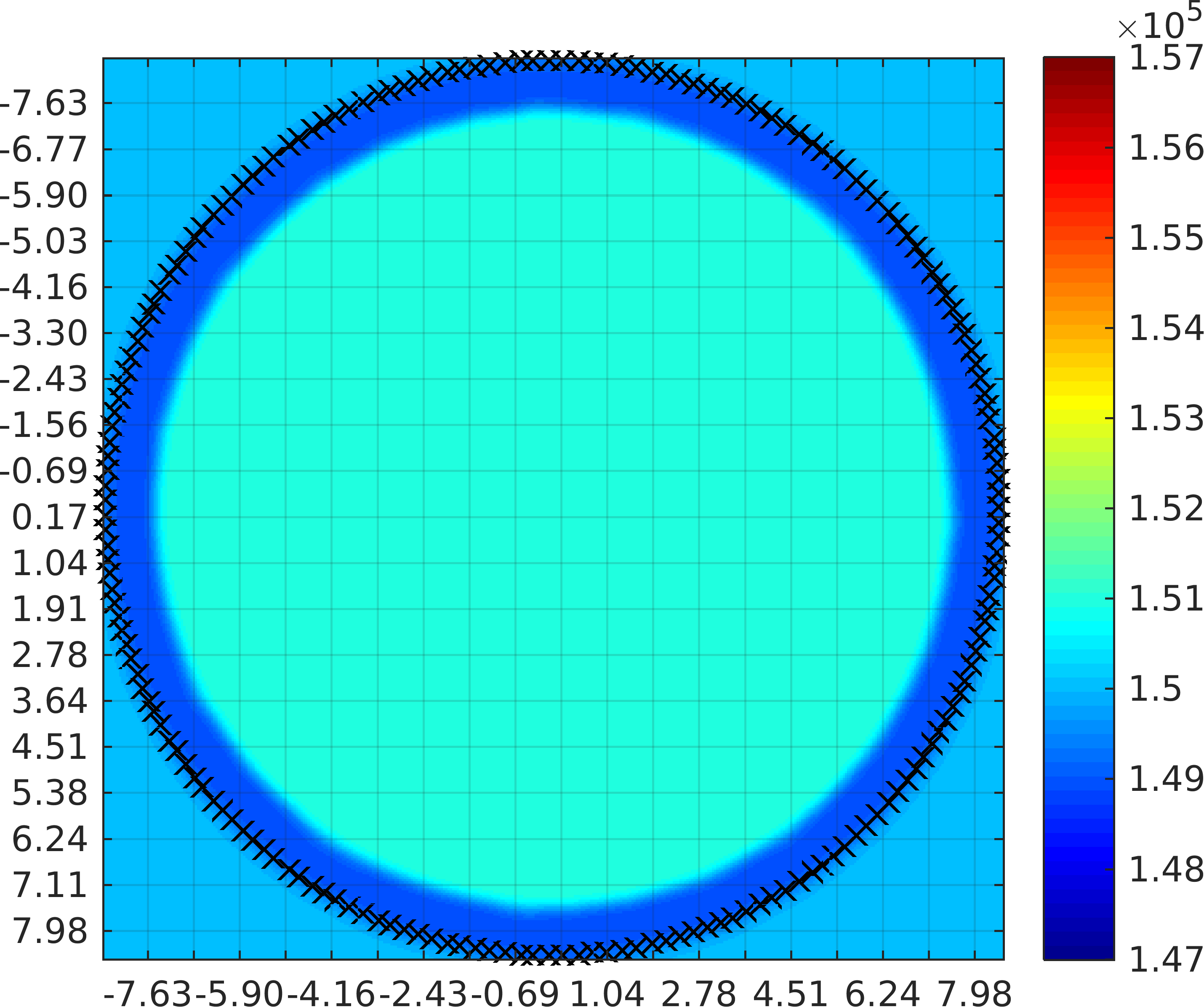 Figure 24
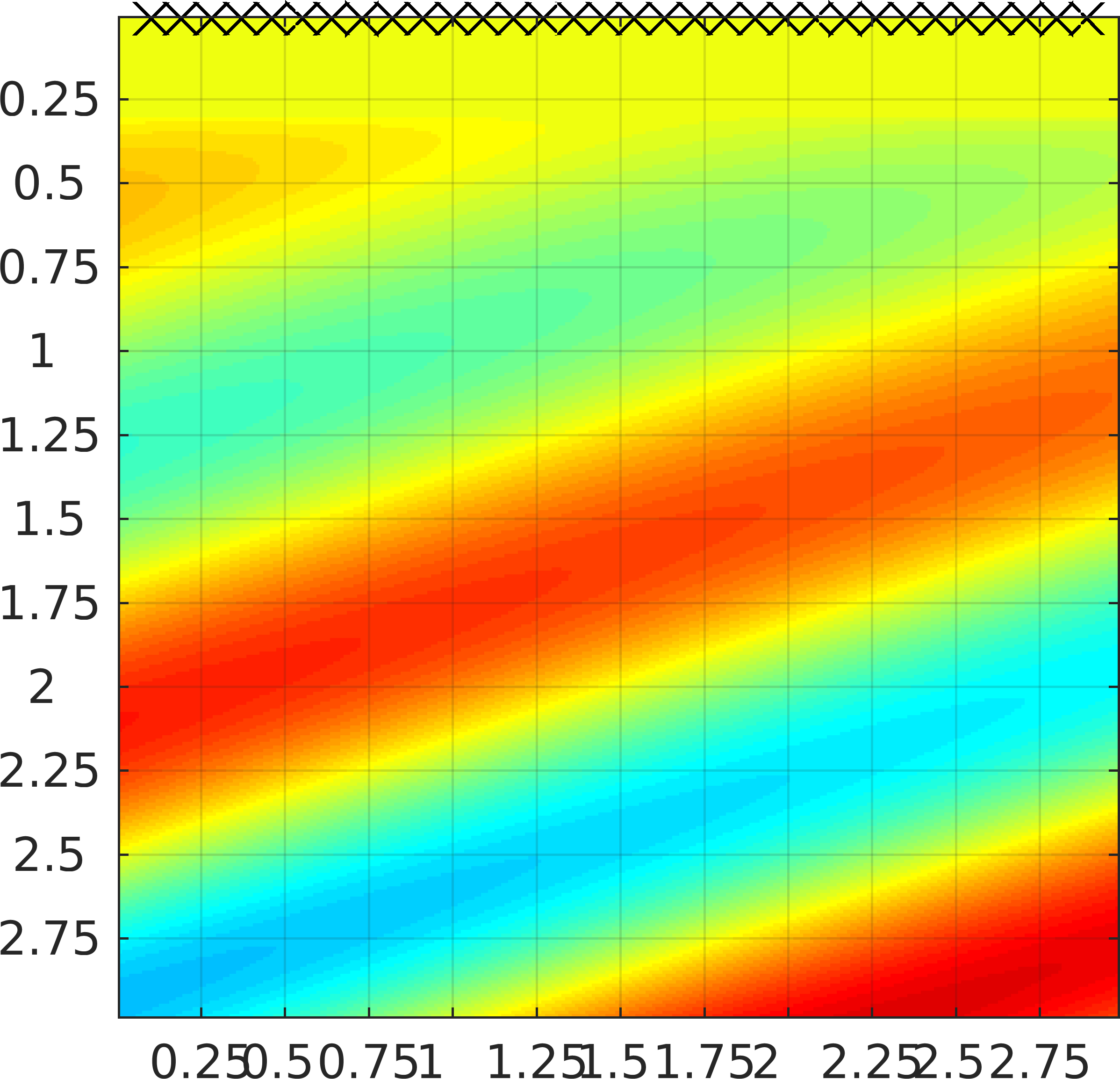 Figure 25
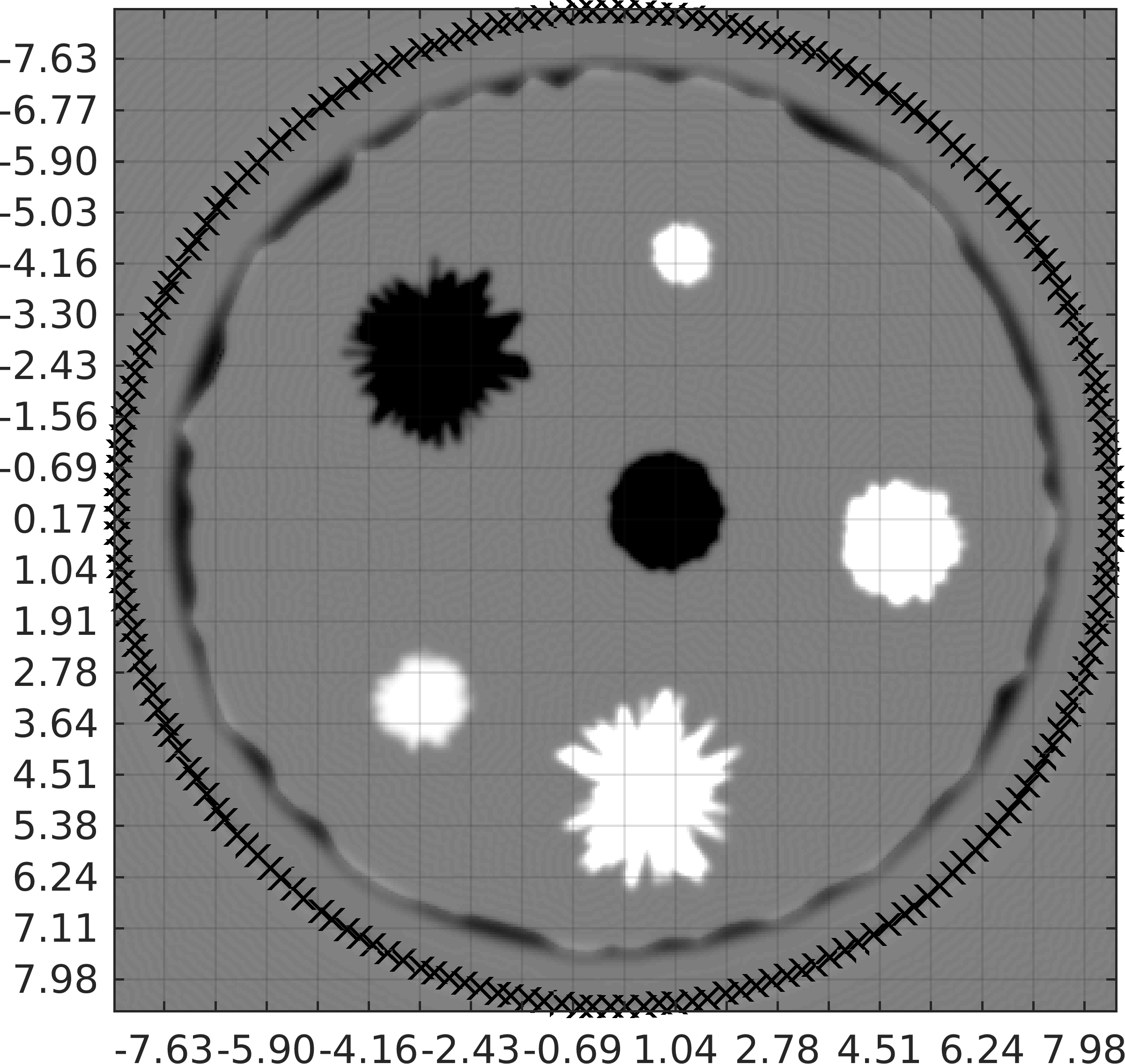 Figure 26
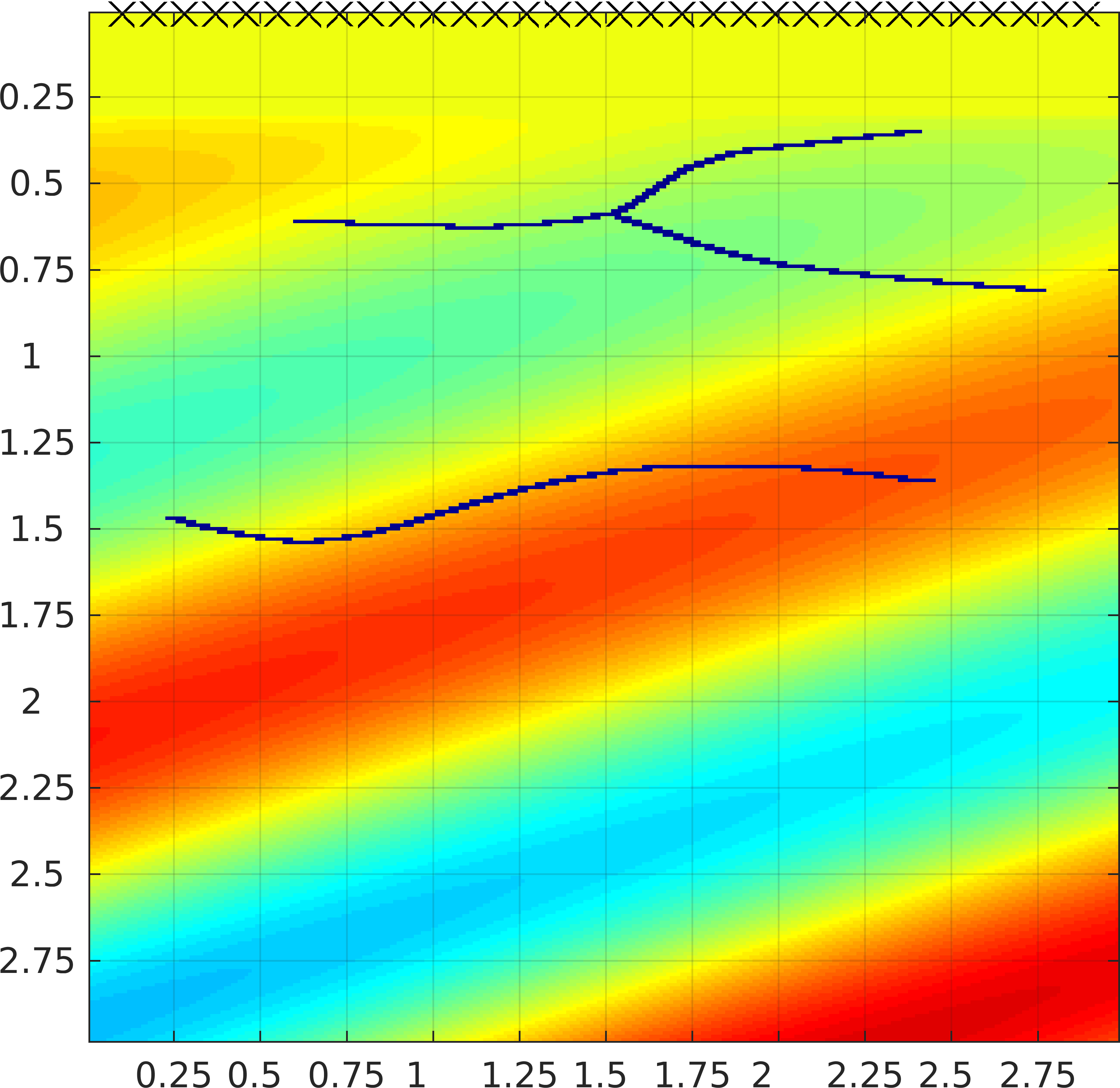 Figure 27
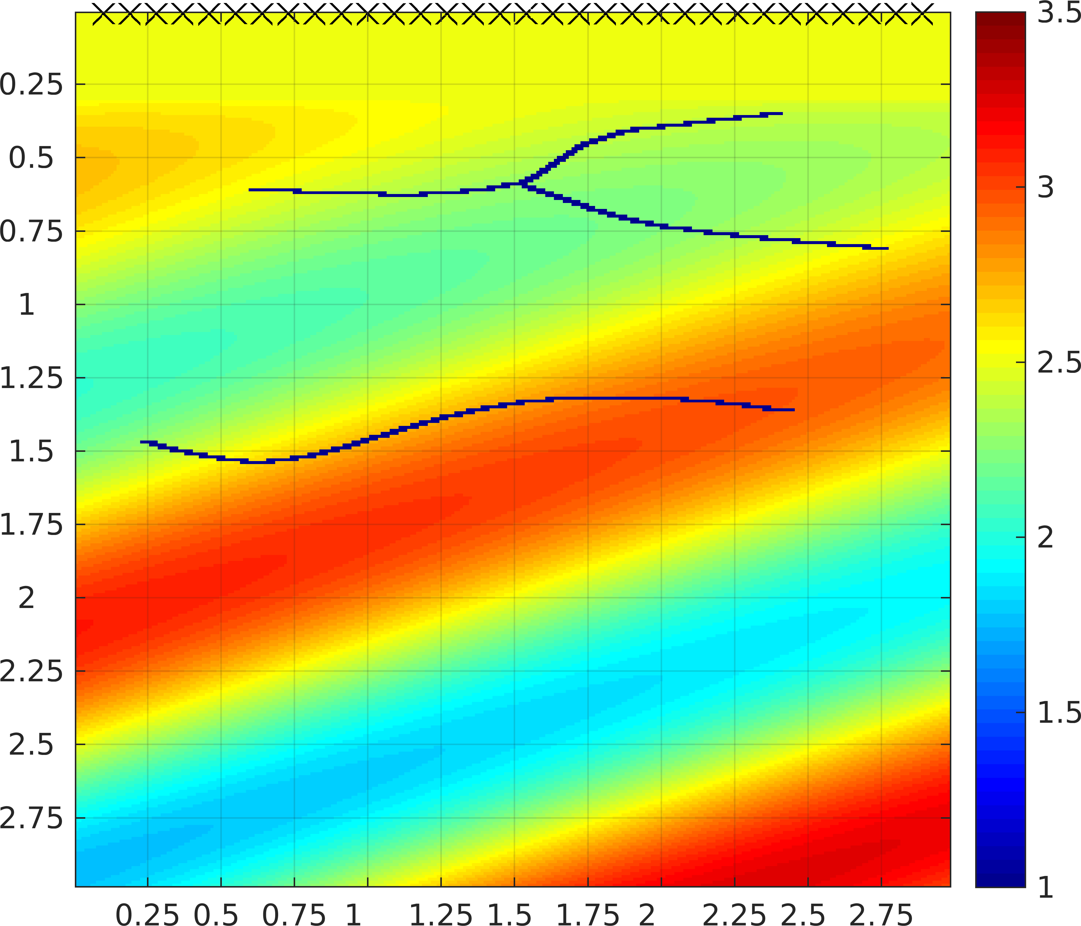 Figure 28
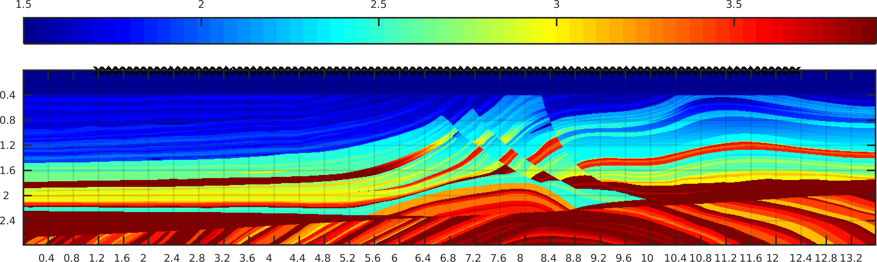 Figure 29
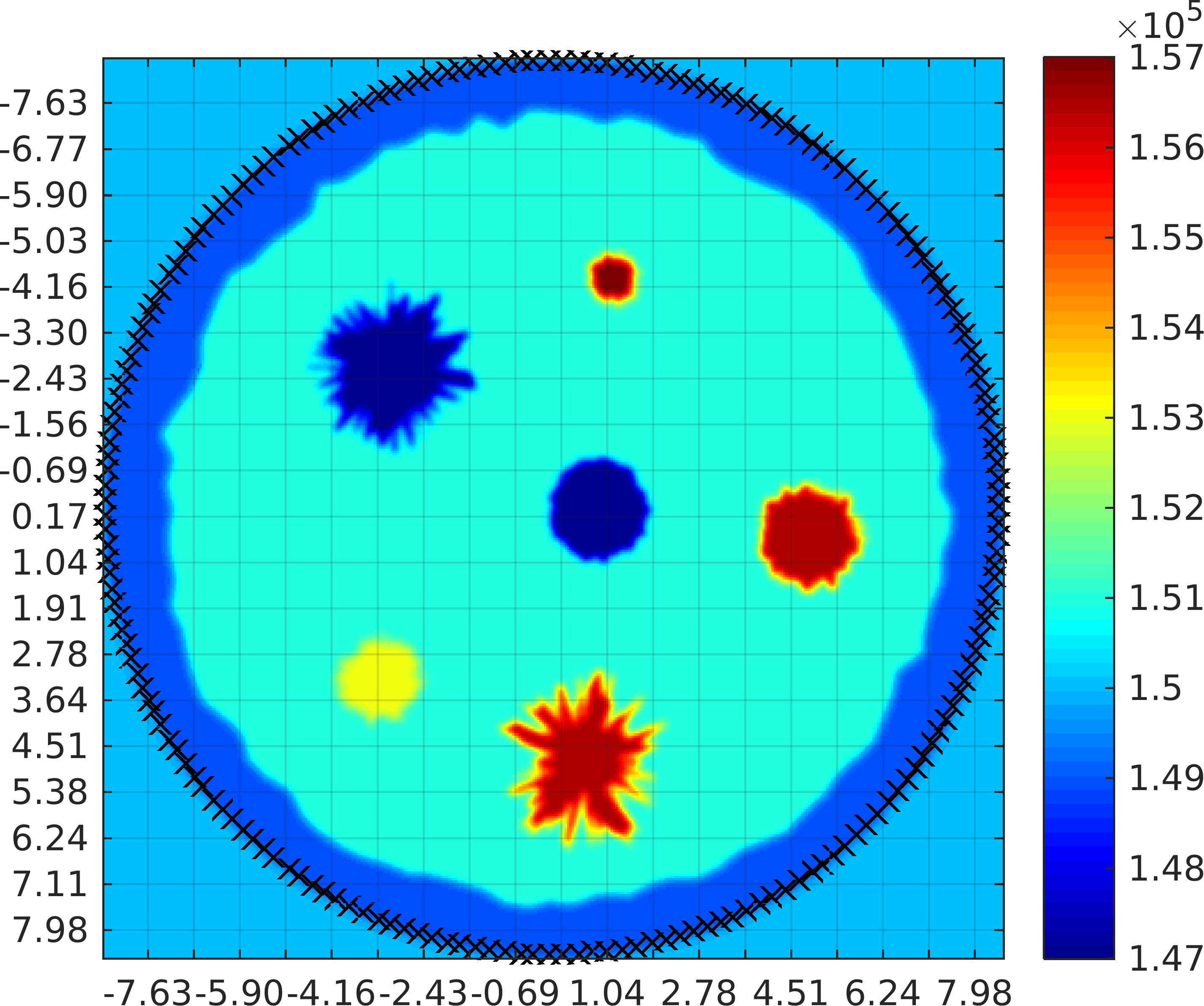 Figure 30
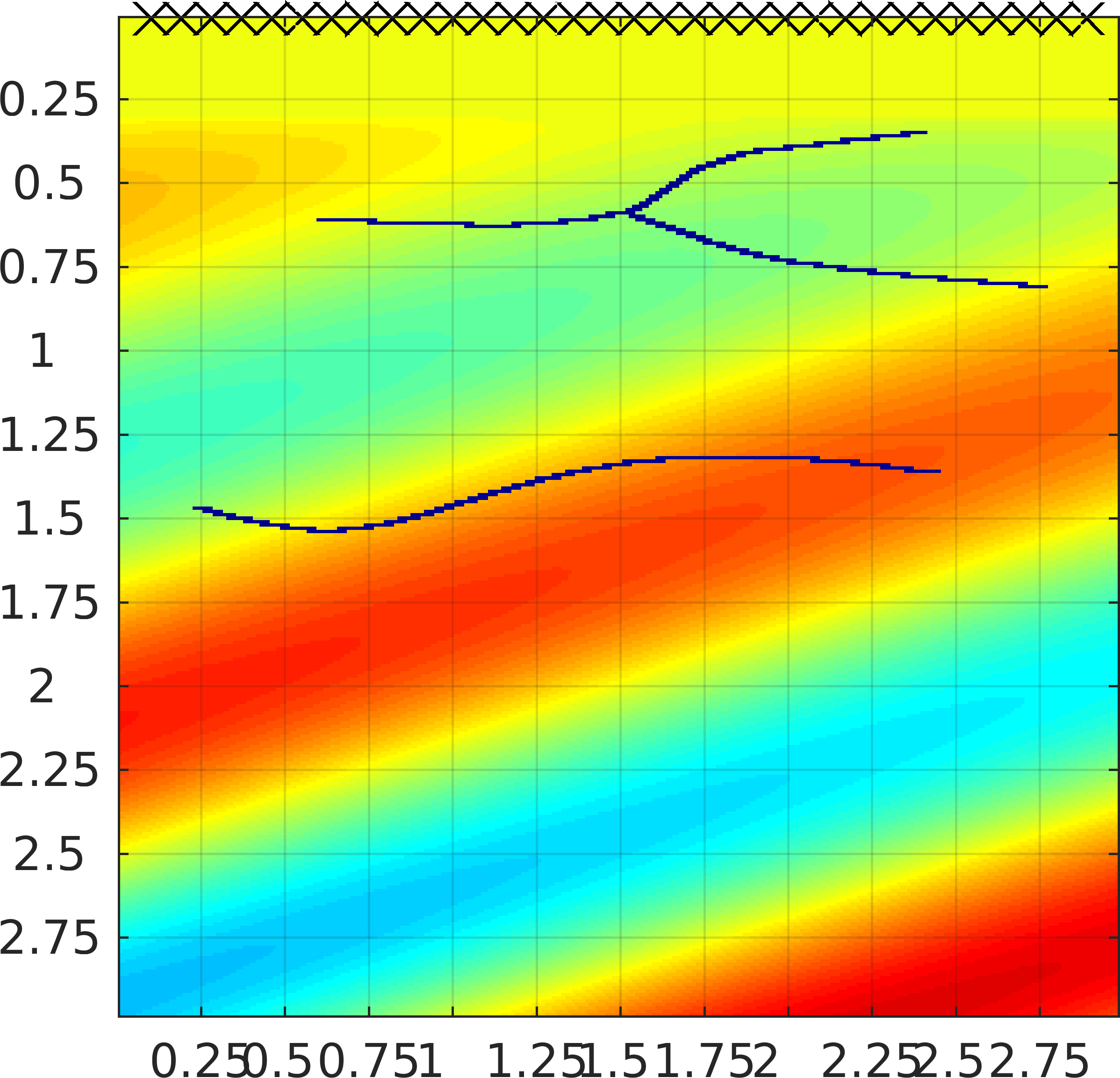 Figure 31
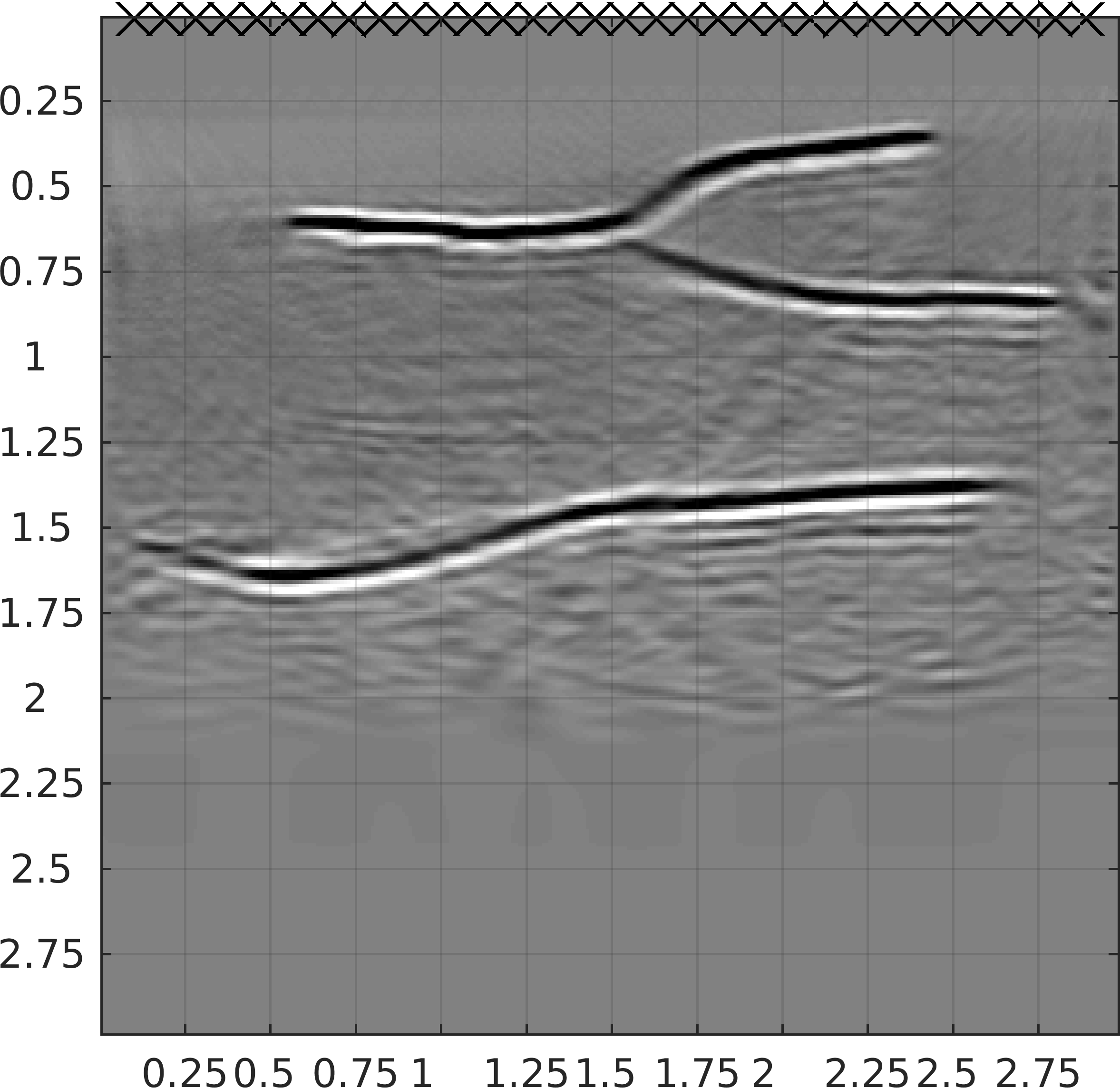 Figure 32
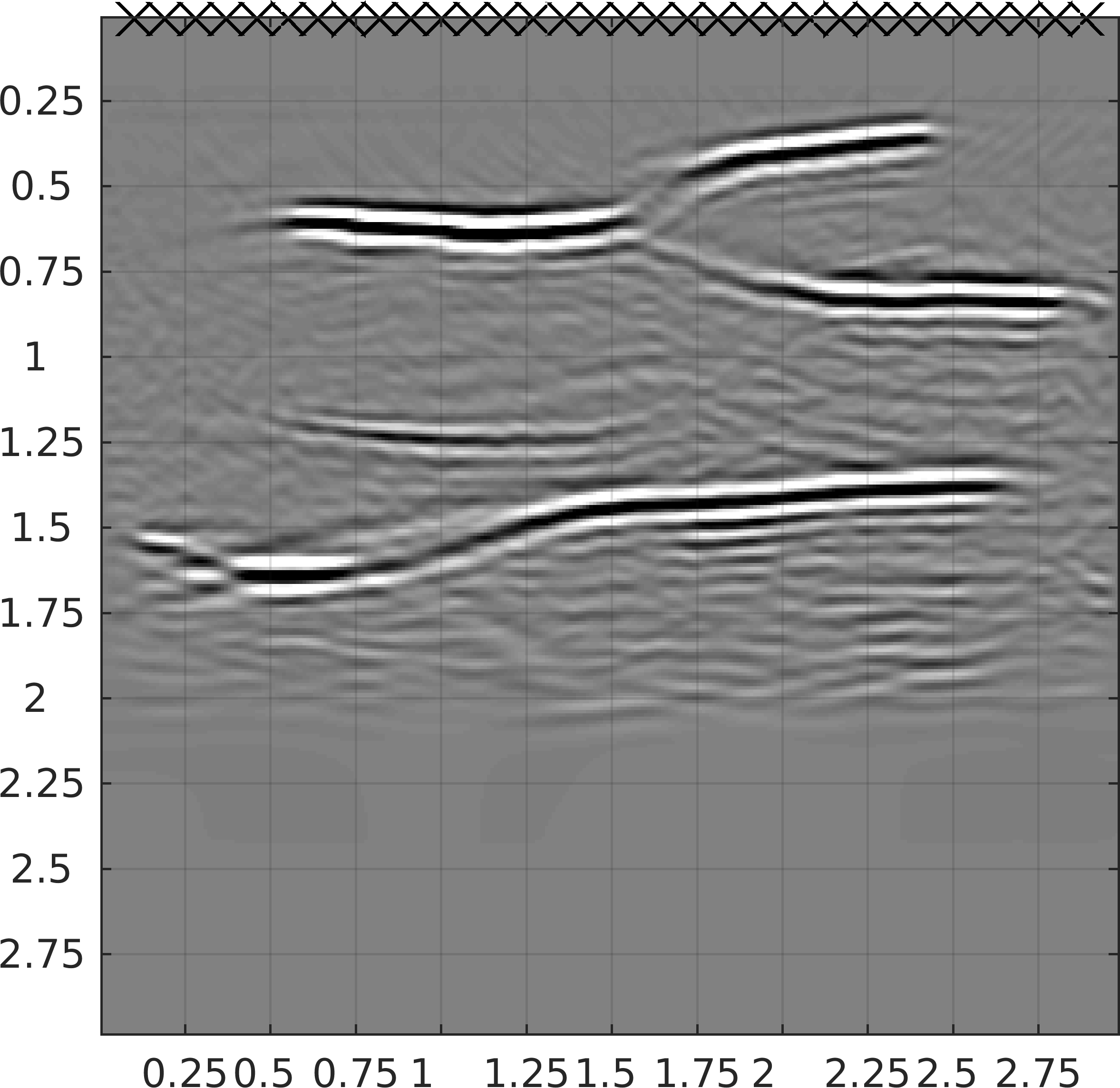 Figure 33
 Figure 34
 Figure 35
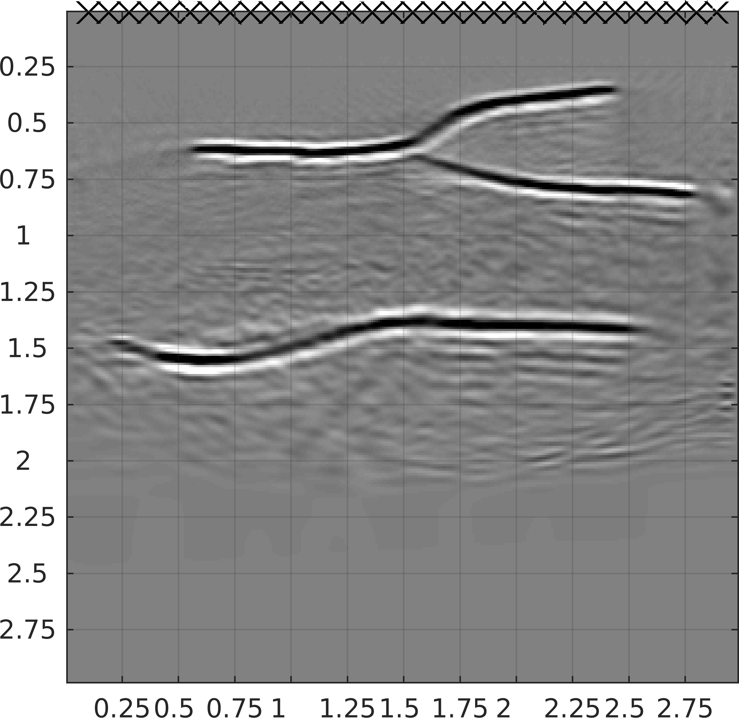 Figure 36
 Figure 37
 Figure 38
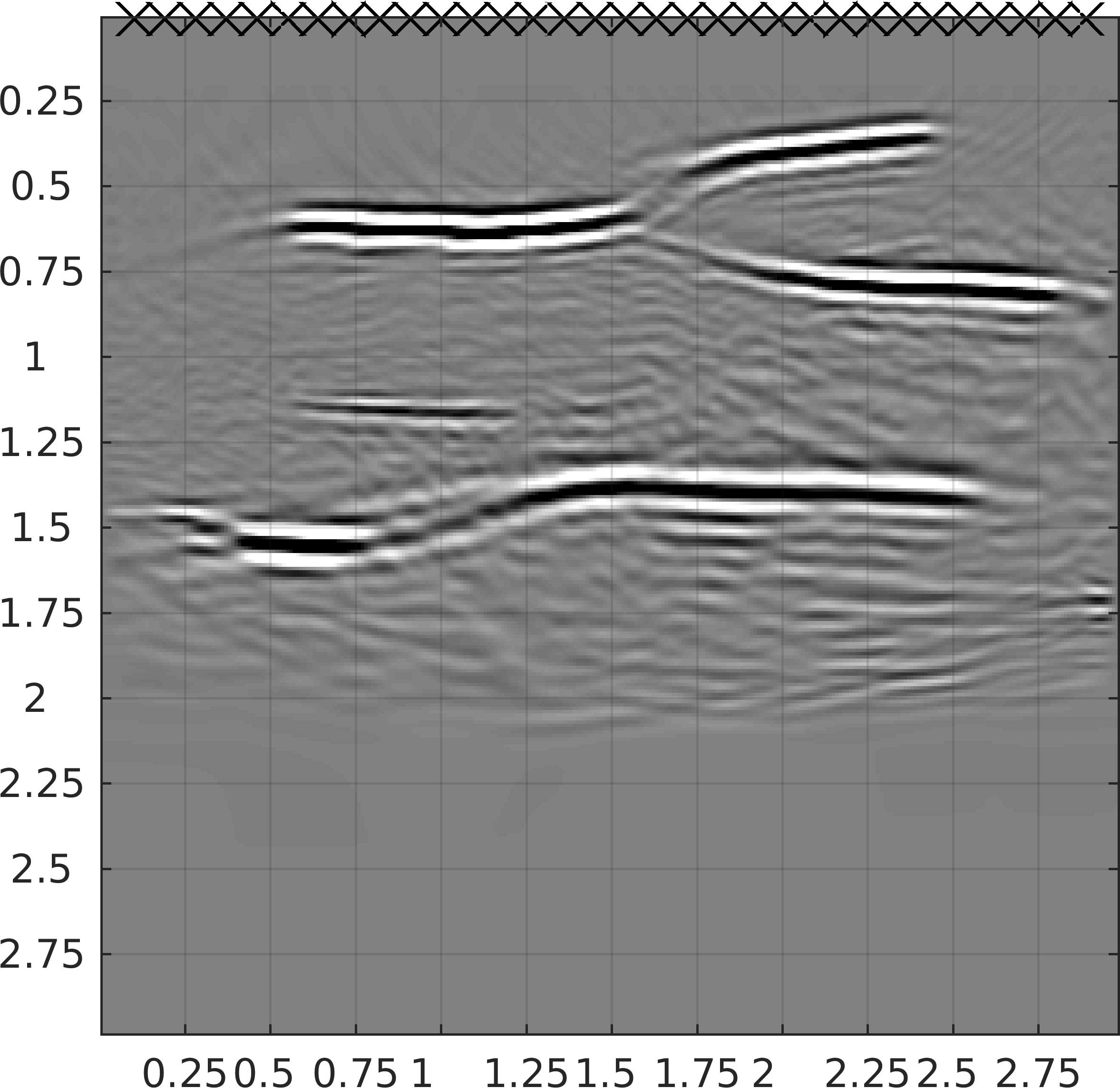 Figure 39
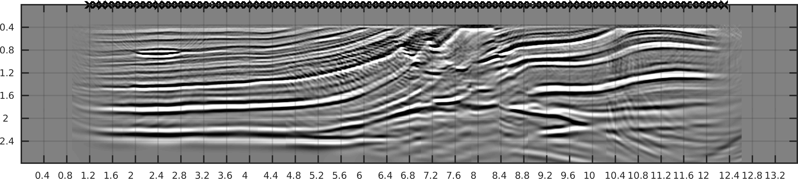 Figure 40
Peer Reviews
No public reviews on file for this paper yet. If you reviewed it on a platform where reviews are public (OpenReview, ICLR, NeurIPS, ICML), you can paste yours below so the community can read it here.
Videos
No videos yet. Explain this paper in a talk, walkthrough, or lecture? Add one.
A nonlinear method for imaging with acoustic waves via reduced order model backprojection
Vladimir Druskin111Schlumberger-Doll Research Center, 1 Hampshire St., Cambridge, MA 02139-1578 USA ()
Alexander V. Mamonov222University of Houston, Department of Mathematics, 3551 Cullen Blvd., Houston, TX 77204-3008 USA () and Mikhail Zaslavsky333Schlumberger-Doll Research Center, 1 Hampshire St., Cambridge, MA 02139-1578 USA ()
Abstract
We introduce a novel nonlinear imaging method for the acoustic wave equation based on data-driven model order reduction. The objective is to image the discontinuities of the acoustic velocity, a coefficient of the scalar wave equation from the discretely sampled time domain data measured at an array of transducers that can act as both sources and receivers. We treat the wave equation along with transducer functionals as a dynamical system. A reduced order model (ROM) for the propagator of such system can be computed so that it interpolates exactly the measured time domain data. The resulting ROM is an orthogonal projection of the propagator on the subspace of the snapshots of solutions of the acoustic wave equation. While the wavefield snapshots are unknown, the projection ROM can be computed entirely from the measured data, thus we refer to such ROM as data-driven. The image is obtained by backprojecting the ROM. Since the basis functions for the projection subspace are not known, we replace them with the ones computed for a known smooth kinematic velocity model. A crucial step of ROM construction is an implicit orthogonalization of solution snapshots. It is a nonlinear procedure that differentiates our approach from the conventional linear imaging methods (Kirchhoff migration and reverse time migration - RTM). It resolves all dynamical behavior captured by the data, so the error from the imperfect knowledge of the velocity model is purely kinematic. This allows for almost complete removal of multiple reflection artifacts, while simultaneously improving the resolution in the range direction compared to conventional RTM.
keywords:
Imaging, wave equation, acoustic, seismic, migration, model reduction, data-driven reduced order model, Krylov subspace, Gram-Schmidt orthogonalization, block Cholesky decomposition
AMS:
86A22, 35R30, 41A05, 65N21
1 Introduction
We consider here a problem of estimating a coefficient of a scalar wave equation, an acoustic velocity, in some domain of interest, from the measurements of its solutions, typically referred to as wavefields, on an array of transducers located on the boundary of said domain. Two aspects of this problem are typically considered. First, a quantitative reconstruction of the coefficient is the subject of the so-called full waveform inversion (FWI) [16, 13, 32]. Second, one may seek a qualitative estimate of the acoustic velocity, say its discontinuities. The discontinuities in the acoustic velocity lead to reflections of waves and thus may be referred to as reflectors or scatterers. The problem of estimating the reflectors (scatterers) from the measurements of the reflected (scattered) wavefields is often referred to as the imaging problem [23, 15, 21]. It is the imaging of reflectors with acoustic waves that is of interest to us here.
The dependency of wavefields on the acoustic velocity is highly nonlinear, which makes both the quantitative and qualitative estimation of the velocity very challenging. Most state-of-the-art imaging methods employed in seismic geophysical exploration and medical ultrasound diagnostics are linear in the recorded data. When more than one reflector is present, first reflections (primaries) from them are typically mixed together with multiply-reflected wavefields (multiples). This creates additional events in the data compared to linearized case with primaries only. Linear imaging methods may interpret these events as extra reflectors that are not present in the actual medium. This creates image artifacts known as multiples in geophysics [31, 33] or reverberation (“comet tail”) artifacts in medical ultrasound [25, 35]. Consequently, complex (and often computationally expensive) data pre-processing techniques are applied to filter the multiple reflection events out of the data before feeding it to imaging algorithms.
Many conventional methods for imaging with waves rely on the time-reversibility of the wave equation. In one form or another they back-propagate the data from the transducers using certain assumptions on the kinematics of the unknown medium. Such approaches are commonly known as migration [28, 18, 3, 14] or time-reversal [17, 11] methods. Here we propose a completely different approach. Instead of propagating the data, we use the theory of model order reduction [2, 1, 22] to construct an approximate wave equation propagator. The approximant is derived to satisfy certain data interpolation conditions, as explained later. If the data is discretely sampled in time, then the reduced order model (ROM) interpolating the data is an orthogonal projection of the propagator on the (Krylov) subspace spanned by the wavefield snapshots taken precisely at the data sampling instants. Computing the projection requires an orthogonalization of wavefiled snapshots to be performed. Since the wavefields are not known inside the domain of interest, the orthogonalization is performed implicitly. It is a nonlinear operation that is crucial to our approach, as it allows to suppress the effects of multiple reflections and probe the medium of interest with localized wavefields.
The use of ROMs in inversion and imaging is not an entirely new idea. Resistor network ROMs were used successfully to obtain quantitative reconstructions of conductivity in two-dimensional electrical impedance tomography (EIT) both directly and iteratively [4, 6, 7, 9, 5]. They were also employed in [10] to reconstruct Schrödinger potentials. While the resistor networks interpolate the EIT or Schrödinger data, they are not ROMs of projection type, unlike the ones considered here. Projection-based ROMs were first studied in the context of inversion for the coefficient of a parabolic equation in [20, 8]. Finally, in [19] reduced models interpolating the time domain wave equation data were introduced to obtain quantitative reconstructions of acoustic velocity. Here we consider ROMs of the same type as in [19], and their construction follows a similar procedure. However, the use of ROMs is different. While in [19] the information about the acoustic velocity is extracted directly from the matrix entries of the ROM, here we perform a backprojection operation on the ROM to go from the reduced model space back to the “physical” space of the domain of interest. This method was first introduced by the authors in a conference abstract [27], and we present here a thorough exposition of the approach briefly outlined therein.
The paper is organized as follows. We begin in section 2 with a forward data model and a formulation of inversion and imaging problems. To simplify the subsequent ROM construction, we symmetrize the data model in section 3. Then we define the time-domain interpolatory ROM and discuss some of its properties in section 4. An algorithm for computing the ROM from the data is given in section 5. After the ROM is computed, we introduce its backprojection and the corresponding imaging functional. Both questions are addressed in section 6. An interpretation of the imaging functional that explicitly separates the kinematic and reflective behavior is given in section 7. A thorough numerical study is performed in section 8. In particular, the orthogonalized wavefield snapshots that span the projection subspace are discussed in section 8.2. Approximations of delta functions by the outer products of orthogonalized snapshots are considered in section 8.3. We compare the proposed ROM backprojection imaging method to conventional reverse time migration (RTM) in section 8.4. Stability of ROM computation in the presence of noise and a regularization algorithm are addressed in section 8.5. The numerical study is concluded in section 8.6 with two large scale synthetic examples from geophysical exploration and medical ultrasound diagnostics. Finally, we conclude in section 9 and discuss the three main directions of future research.
2 Problem formulation
Consider a scalar wave equation for the acoustic pressure
[TABLE]
where is the domain of interest in , . Domain can be either infinite or finite. Here we assume is finite with boundary split into the accessible and inaccessible parts respectively. We also assume that the acoustic velocity is piecewise smooth in .
Wave equation (1) is driven by the source term comprised of a wavelet , source weighting function and a distribution . Source distribution is supported on the accessible boundary
[TABLE]
and is defined so that
[TABLE]
for any smooth test function , where is the surface element (arc length in the case ) at point .
Since (1) is defined for all , we enforce a decay condition for large negative times
[TABLE]
We prescribe reflective boundary conditions on the accessible boundary
[TABLE]
where is the unit outward normal at . We also prescribe zero Dirichlet conditions on the inaccessible boundary
[TABLE]
although zero Neumann conditions can be used instead.
Following [19] we assume that the source wavelet is an even, sufficiently smooth approximation of with a non-negative Fourier transform
[TABLE]
To simplify the exposition we assume that different sources correspond to varying and , while the wavelet remains the same, i.e. each source emits the same waveform.
All possible sources and receivers on provide the knowledge of the boundary measurement operator
[TABLE]
for all and satisfying (2).
To simplify the exposition it is beneficial to move the source term to the initial condition using a form of Duhamel’s principle, as explained in [19]. Using (7) and the fact that is even, we can work instead of the pressure with its even part
[TABLE]
It satisfies a homogeneous wave equation
[TABLE]
with initial conditions
[TABLE]
where we denote by the spatial part of the PDE operator in (10):
[TABLE]
The homogeneous boundary conditions (5)–(6) remain unchanged
[TABLE]
The knowledge of boundary measurement operator implies the knowledge of another operator
[TABLE]
In practice, we do not have the full knowledge of the boundary measurement operator . Instead, we take a finite sampling of it in both space and time.
First, consider the spatial measurement sampling. We place transducers on the accessible boundary that act simultaneously as sources and receivers. The corresponding source-receiver distributions are , with disjoint supports
[TABLE]
Since the supports are disjoint, we fix single source and receiver weighting functions and respectively. Their particular choice is discussed in section 3. Then the continuum time data that we can in principle measure with such transducer set-up is an matrix-valued function of time
[TABLE]
which can also be written using (3) and (14) as
[TABLE]
where satisfies initial conditions (11) with . Hereafter we denote matrices and matrix-valued functions by bold letters. Physically, the entry is the signal recorded at receiver at time while the medium is excited with source .
Second, in practice the temporal measurements are also sampled discretely at a certain rate. As explained later, our method relies on the temporal sampling being uniform. Hence, we introduce time instants , , where denotes the sampling interval and the total number of temporal samples is .
Once the measurements are sampled in both space and time, we can define the sampled data as
[TABLE]
We are now in position to state the following two problems.
Inversion problem. Given measured data (18) estimate the acoustic velocity in .
Imaging problem. Given measured data (18) and a smooth kinematic velocity model estimate the (location of) discontinuities of the acoustic velocity .
In [19] a method to solve the inversion problem in one dimension and its generalization to higher dimensions was considered. The method relies on the techniques of model order reduction. Here we use similar techniques to address the imaging problem. Unlike the quantitative inversion problem, where no a priori knowledge of the acoustic velocity is available, the imaging can be viewed as a problem of qualitative estimation of the velocity discontinuities on top of a known kinematic background. By referring to as the kinematic model or background, we assume that it captures sufficiently well the kinematics of the wave equation (10), i.e. the wave travel times between pairs of points in are approximately equal for and .
3 Symmetrized data model
Our imaging approach relies on the construction of a reduced order model of the sampled data (18). In order to understand the form which such a model has to take, it is beneficial to transform (17) and (18) further.
Denote by the solution of (10) with initial conditions
[TABLE]
i.e. the wavefield induced by source . In what follows it is convenient to work simultaneously with the wavefields induced by all sources. Thus, we define a row-vector-valued function of time by
[TABLE]
which solves
[TABLE]
where the action of operators on row-vector-valued functions is understood component-wise.
The initial conditions for (21) are
[TABLE]
with
[TABLE]
Using operator functions we can write the solution of (21) with initial conditions (22) as
[TABLE]
In the derivations below it is convenient to use the following notation for products of row-vector-valued functions. Suppose then by we denote
[TABLE]
where
[TABLE]
Then using (25) we can write (17) in matrix form as
[TABLE]
We notice that in (27) there is a certain asymmetry between the source and receiver terms. Since the sources and receivers are collocated, it is possible to transform (27) to a symmetric form which makes the subsequent derivation of the reduced model much simpler. To achieve this we introduce the symmetrized PDE operator
[TABLE]
a similarity transform of , since . Using the facts that operator functions of commute and that the Fourier transform of the source wavelet is non-negative (see section 2) we can rewrite (27) as
[TABLE]
To transform further we observe that similarity transforms commute with analytic operator functions, thus
[TABLE]
To write (30) in a fully symmetric form we need to make the following assumption on the source and receiver functions, namely
[TABLE]
for some known function . Since the source and receiver functions are always multiplied by distributions supported on the accessible boundary, assumption above only requires the knowledge of the acoustic velocity on which is not restrictive. Indeed, if one has access to to place the transducers, it should be possible to determine there as well.
Under assumption (31) we obtain the expression for the continuum time data in a fully symmetric form
[TABLE]
where
[TABLE]
is the row-vector-valued transducer function .
Note that is self-adjoint with respect to the standard inner product (26), and so are its operator functions including the one in (32). Since the transducer function enters (32) in a symmetric fashion, the continuum time data is also self-adjoint
[TABLE]
which is known as reciprocity, i.e. the data measured at receiver induced by source is the same as data measured at receiver induced by source .
4 Time-domain interpolatory reduced order model
At the core of our imaging approach is the construction of a reduced order model for the sampled data , . To that end we need to transform the symmetrized data (32) using the fact that the data is sampled uniformly in time. Specifically, since
[TABLE]
we can write
[TABLE]
where are Chebyshev polynomials of the first kind of degree and is the propagator
[TABLE]
We seek the reduced order model in the form (36), namely
[TABLE]
where is the reduced order propagator and is the reduced order transducer matrix.
To compute the reduced order propagator and transducer matrices we solve the following interpolation problem
[TABLE]
Note that since there are transducers, reduced order matrices and consist of blocks. In particular, consists of blocks, while is a block column matrix blocks tall. This allows to use block versions of results in [19] on the existence and construction of the solution to (39). This requires defining the following quantities.
First, following the procedure of section 3 we introduce the row-vector-valued function of symmetrized wavefields as solutions of
[TABLE]
with initial conditions
[TABLE]
Second, since the data is sampled uniformly in time, we also sample the symmetrized wavefields to obtain the symmetrized snapshots
[TABLE]
Obviously, the sampled data in terms of the symmetrized snapshots is given by
[TABLE]
Third, we introduce the following block Krylov subspace
[TABLE]
where by “block” we refer to the fact that each , is a row-vector-valued function of and thus the dimension of is . We can consider an orthonormal basis for (44) that we denote by , which we write as
[TABLE]
The basis is orthonormal in the sense of the following “matrix” product. Let be
[TABLE]
then
[TABLE]
where each is defined by (25) with the distinction that , do not depend on . The role of time is played by the indices and once the temporal sampling (42) is introduced. Then we can write the orthonormality conditions for as
[TABLE]
where and are identity matrices of sizes and respectively.
Now we can address solving interpolation problem (39) to obtain the reduced model , . The solution is characterized by the following lemma.
Lemma 1**.**
Reduced order propagator and transducer matrix that solve the interpolation problem
[TABLE]
are orthogonal projections
[TABLE]
of the true propagator (37) and transducer function (33) on Krylov subspace (44), where is an orthonormal basis for in the sense of (48), and the products in (50) are understood in the sense of (46)–(47), in particular
[TABLE]
The proof of the lemma is in Appendix A. We make the following observations regarding Lemma 1 the implications of which are addressed in detail in the subsequent sections.
Not surprisingly, in order to match the data at time instants , we project on the subspace of wavefield snapshots sampled at the same instants . However, the Krylov subspace is spanned by only snapshots, while the data is sampled at instants. This question is addressed in the proof in Appendix A.
We observe that and are not unique as defined by (50). This ambiguity comes from the choice of an orthonormal basis in . If and are solutions of (49) then and are also solutions for any unitary . We make use of this fact in the proof in Appendix A.
However, not all orthonormal basis choices are equally useful if one wants to use the reduced model for imaging (or inversion, see [19]). Inversion and imaging applications require the basis functions to be localized in which implies a certain structure of and . The exact structure of and is established in Lemma 4 in section 5.
While (50) characterizes the solution of (49), it does not provide a practical way of computing and . Indeed, it requires the knowledge of which comes from orthogonalization of symmetrized wavefield snapshots , . Obviously, when solving inversion and imaging problems we do not have the knowledge of for . The only measurements we make are those of , . Thus, we must find a way to compute projections (50) from the knowledge of the sampled data only. Algorithm 2 achieving that is derived in section 5.
5 Reduced order model computation
Let us introduce the following row-vector-valued function of symmetrized snapshots
[TABLE]
so that .
If we had the knowledge of , then one way to compute an orthonormal basis for is to apply block Gram-Schmidt orthogonalization procedure to . In matrix notation this can be written as a block QR decomposition
[TABLE]
where is a block lower triangular matrix
[TABLE]
with blocks . Note that multiplication of by a matrix from the right follows the standard rules of matrix multiplication.
While we do not have the knowledge of , relation (53) implies that
[TABLE]
which is a block Cholesky decomposition of the mass matrix
[TABLE]
The advantage of (56) over (53) is that it does not require the knowledge of wavefield snapshots in , but only the inner products between them.
Recall from (42) that the snapshots are expressed in terms of Chebyshev polynomials as . On the other hand, the products of Chebyshev polynomials satisfy
[TABLE]
and so the inner products between the snapshots are given by
[TABLE]
Combining (42) and (43) the data is , hence the blocks of the mass matrix can be expressed just in terms of the sampled data
[TABLE]
where , . Thus, in order to compute the block Cholesky factor of only the knowledge of the sampled data is required.
Note that the mass matrix notation for the Gramian that we use is not a coincidence. Indeed, if we want to approximate (42) on the Krylov subspace (44) with a Galerkin method, is the mass matrix and we can also define the stiffness matrix
[TABLE]
which we can also express in terms of the sampled data.
Let us consider the action of the propagator on the snapshot :
[TABLE]
i.e. takes the average of the symmetrized wavefield propagated by time forward and backward. Now we combine (61) with (42) and (57) to express the blocks of the stiffness matrix in terms of the sampled data
[TABLE]
where , .
Formulas (59)–(62) enable us to compute the reduced model , from the knowledge of the sampled data only. Indeed, for the reduced order propagator from (50) and (53) we obtain
[TABLE]
Similarly, for the reduced order transducer matrix
[TABLE]
We summarize the derivations above in the following algorithm.
Algorithm 2** (Reduced order model computation from sampled data).**
Given the sampled data , , to compute the reduced order propagator and transducer matrix that solve the interpolation problem
[TABLE]
perform the following steps:
Form the mass matrix consisting of blocks for according to
[TABLE] 2. 2.
Form the stiffness matrix consisting of blocks for according to
[TABLE] 3. 3.
Perform block Cholesky decomposition of the mass matrix
[TABLE]
to compute the block lower triangular Cholesky factor . 4. 4.
Compute and from
[TABLE]
Note that while the regular Cholesky factorization is defined uniquely, there is an ambiguity in defining block Cholesky factorization that comes from the computation of diagonal blocks . The particular version of block Cholesky algorithm that we use to compute (68) is given below.
Algorithm 3** (Block Cholesky decomposition).**
*To compute block Cholesky decomposition of a matrix with blocks, perform the following steps:
For *
[TABLE]
For
[TABLE]
Other choices can be used instead of (70) to compute the diagonal blocks , as long as they satisfy
[TABLE]
For example, one may use eigendecomposition or regular Cholesky factorization of the right hand side of (72) to obtain . No matter the choice, the reduced order propagator obtained by Algorithm 2 has the structure established in the following lemma.
Lemma 4**.**
Reduced order propagator computed by Algorithm 2 has a block tridiagonal structure
[TABLE]
while the reduced order transducer matrix has the structure
[TABLE]
where , .
The proof is given in Appendix B. Here we note that since defined by (63) is self-adjoint, so are its diagonal blocks , .
6 Backprojection imaging functional
Once the reduced order propagator is computed from the sampled data with Algorithm 2, we can use it for inversion and imaging. In order to construct an imaging functional from , we consider first the Green’s function for the symmetrized problem (40)–(41). Then satisfies
[TABLE]
with initial conditions
[TABLE]
where we denote by a delta function concentrated at .
Then similarly to (24) we can formally write the solution to (75)–(76) at time as
[TABLE]
in terms of the inner product (26). Alternatively, if we treat and as row-vector-valued functions with a single column, then we can use the notation of (25) to write
[TABLE]
If we could probe the propagator with delta functions, this would allow us to image the Green’s function (78). This is not possible if we only have access to the sampled data and thus to . However, we can probe with other functions. Let us consider
[TABLE]
a function of two variables
[TABLE]
As we will see later, approximates in a certain sense. Thus, we introduce an approximate Green’s function
[TABLE]
by replacing the delta functions in (78) with . Then we can transform
[TABLE]
or explicitly
[TABLE]
where the standard rules for matrix-vector multiplication apply.
While can be computed from the sampled data, it is not possible to obtain the orthonormal basis functions from the knowledge of only. Thus, we need to make another approximation in (82)–(83). Recall that when solving an imaging problem we are given the approximate knowledge of the travel times between pairs of points in in the form of a smooth kinematic model . For we can compute the symmetrized wavefield snapshots in the whole domain , as well as their orthogonalization
[TABLE]
and the projected propagator
[TABLE]
Hereafter we use the subscript to refer to all quantities associated with including the Green’s function and its approximation defined in (81).
If approximates the kinematics of the problem with unknown desired sufficiently well, we may expect that the orthogonalized snapshots for the two problems are also close
[TABLE]
Particular reasons for expecting such behavior are discussed later. Then we can make another approximation in (81)–(82) to obtain
[TABLE]
where all terms can be computed either from the knowledge of the sampled data or the kinematic model.
Finally, we have all the components to define the ROM backprojection imaging functional
[TABLE]
that approximates the difference between the Green’s functions for the unknown medium and the kinematic model , that is
[TABLE]
If in the vicinity of a point the unknown medium contains a reflector, then the difference (89) will be large. Otherwise, and .
The use of term “backprojection” should not be confused with the classical method in computed tomography [26]. The (filtered) backprojection formula for inversion of Radon transform in computed tomography is linear in the input data, while the computation of from the data , in Algorithm 2 is a highly nonlinear procedure due to block Cholesky factorization (68) and inversion (69).
7 Interpretation in terms of Schrödinger wave equation
Here we present an interpretation of the imaging formula (88) that goes beyond the approximate Green’s function perturbation (89). Note that the imaging procedure in section 6 makes a distinction between the kinematic part of that is assumed to be well approximated by , and the reflective part of that is imaged by . Meanwhile, the operator (12) has a single coefficient that does not allow for a clear separation between the kinematic and reflective parts. Thus, instead of the wave equation (10) with operator (12), in a slight abuse of notation we consider the wave equation
[TABLE]
with operator
[TABLE]
where is the wavespeed and is the acoustic impedance.
The operator (91) is symmetric with respect to the -inner product and nonnegative definite (positive definite for a bounded ). Thus, following section 3 we use to transform (90) into where the symmetrized operator is given by
[TABLE]
Furthermore, we can transform to Schrödinger form
[TABLE]
with
[TABLE]
and the Schrödinger potential
[TABLE]
where we omit the dependency on of , and to simplify the notation.
To obtain the separation between the kinematic and reflective parts we assume that the wavespeed is known exactly and we only image the perturbations of the Schrödinger potential
[TABLE]
where is the known background impedance. Note that the knowledge of is a rather reasonable assumption. Discontinuities of do not produce significant reflections observable for moderate apertures [29, Chapter 6], so typically the inexactness of does not introduce significant topological errors in the image, and may only result in a slight image deformation.
Similarly to (75) we introduce the Green’s functions and for the unknown and reference media respectively. They solve
[TABLE]
where , and {\mathcal{C}}_{o}=\sqrt{c_{o}}\nabla\cdot\Big{(}c_{o}\nabla\sqrt{c_{o}}\Big{)}.
According to (89) the functional is related to the perturbation
[TABLE]
It follows from (97)–(98) that it satisfies approximately
[TABLE]
if we assume
[TABLE]
If we also introduce the Green’s function solving
[TABLE]
we can express the solution of (100) as
[TABLE]
and so
[TABLE]
Thus, due to causality of (98) and (102), yields averaged in the travel time ball of radius centered at . Note that since (104) only relies on the solutions of (100) for , the assumption (101) is valid for small enough compared to the scale of inhomogeneities of (and thus ).
8 Numerical study and discussion
The proposed imaging method differs significantly from existing approaches. In this section we illustrate numerically and discuss its various aspects that distinguish it from conventional methods.
8.1 Numerical model
To study the performance of the proposed imaging method we consider the following numerical model. Let . The inaccessible boundary consists of the left, right and bottom sides of the square, while is the top side. The accessible boundary supports point-like transducers, i.e.
[TABLE]
where , are the transducer locations.
We use an acoustic velocity model consisting of a smooth background and two extended reflectors one of which is branching. The smooth part of is used as the kinematic model . Both and are shown in Figure 1. Reflectors are relatively high contrast with velocity of inside the reflecting inclusion, while the surrounding background velocities are about depending on the location.
The wave equation is discretized with second order finite differences on a uniform tensor product grid with nodes spaced apart. Each of the two reflectors has thickness of , two grid nodes.
The source wavelet is chosen so that its Fourier transform (7) is
[TABLE]
where determines the characteristic duration of the source wavelet in time. As discussed in [19], it is essential for the stability of ROM computation for the temporal sampling interval to be consistent with the Nyquist sampling limit for the source wavelet. Since the Gaussian (106) does not have a sharp frequency cutoff, its Nyquist limit is not precisely defined, but the choice works well in practice. In particular, in all numerical examples in this section we take . While it is mostly pointless to talk about the “frequency” of the broadband (infinite-bandwidth) source wavelet (106), we can characterize the source in terms of the sampling frequency . Here . The data is measured at time instants , with a terminal time of .
8.2 Orthogonalized wavefield snapshots
At the heart of our imaging approach is the implicit orthogonalization of the symmetrized wavefield snapshots , . This is an essentially nonlinear operation (due to the nonlinearity of block Cholesky factorization in (68) and Cholesky factor inversion in (69)) that makes possible accounting for such nonlinear phenomena as multiple reflections, as discussed later. Wavefield snapshots for the true medium and the kinematic model as well as their orthogonalized counterparts are shown in Figure 2. The following features can be observed.
First, when comparing orthogonalized snapshots to (and also to ) we observe the focusing in both the range and cross-range. Hereafter we refer to the direction orthogonal to the transducer array as the range and to the direction along the array as the range. The orthogonalized snapshots have a well pronounced peak below the corresponding source (up to the lateral bending of the wavefront due to variations). This peak becomes wider as the propagation time increases, i.e. we observe cross-range defocusing which is the consequence of the decrease of effective aperture as the wave travels away from the transducer array.
Second, a phenomenon closely related to focusing that can only be observed in the reflecting medium is the suppression of reflections in the orthogonalized snapshots . While the energy is spread out over reflections in , after orthogonalization the wavefield is concentrated around the peak of . This is an essential feature of the approach, since it allows to suppress the artifacts caused by multiple reflections that conventional linear imaging methods are unable to handle. No matter how complex the reflections in the true medium are, the propagator is probed in (63) with focused orthonormal basis functions that are localized around the same locations as . Note that the presence of reflections can actually improve the focusing, as we can see comparing to in Figure 2.
8.3 Approximations of delta functions
The imaging functional (88) can be written as
[TABLE]
which according to (77) and (89) should approximate
[TABLE]
Thus, in order for the imaging method to work, the following approximations of delta functions must hold
[TABLE]
Given the focused nature of orthogonalized snapshots observed in section 8.2, we expect that their “outer products” in (109) will be well localized, as expected from good approximations of delta functions. This conjecture is explored in Figure 3, where we plot and for a few fixed points as functions of . We observe indeed that both and are well localized and have a clearly pronounced peak for while being close to zero elsewhere. Moreover, we note that the focusing of the outer products and is much tighter than that of the orthogonalized snapshots .
The outer products can be seen as nonlinear analogues of point spread functions quantifying the resolution of the imaging functional . The nonlinearity comes in as dependency of in on the true medium . Note though that the dependency is kinematic in nature, that is if captures the kinematics of the true medium , we expect
[TABLE]
as observed in Figure 3.
8.4 Images and comparison to reverse time migration
Once the focusing and localization properties of orthogonalized snapshots and their outer product are established, we can finally assess the performance of the backprojection imaging functional on the model described in section 8.1 (see Figure 1). We compare our approach with reverse time migration (RTM) [3], a linear imaging approach that is the standard method for high quality imaging with waves in geophysics [14, 30, 34]. Here we use a particular version of RTM known as pre-stack migration, which is more accurate than the computationally cheaper post-stack migration. The pre-stack RTM imaging functional is hereafter referred to as .
Note that both and imaging functionals produce weaker images of reflectors that are further away from the array. This is particularly pronounced when the wave has to pass through reflectors closer to the array before reaching the far ones, thus losing energy in the process, as it gets reflected back to the array at each interface. To account for this behavior, in what follows we modify both imaging functionals by scaling them with a multiplier that depends linearly on the distance from the imaging point to the transducer array. In a slight abuse of notation we still refer to such modified functionals as and .
In Figure 4 we compare the images obtained with ROM backprojection formula (88) and with conventional pre-stack RTM for the model described in section 8.1 with two kinematic models: a kinematic model from Figure 1 consisting of the true smooth background without the reflectors; and a constant kinematic model with . We observe that in both cases our approach is clearly superior compared to its conventional linear counterpart. The main advantage of backprojection imaging is the automatic removal of multiple reflection artifacts. These artifacts appear inevitably in any linear imaging method due to the interaction of reflectors with reflective boundaries (here mainly with the top part of the boundary) and with each other. Each such interaction produces additional events in the data that linear migration methods image as extra reflectors that are not actually present in the true medium. We observe in Figure 4 that the RTM image has many such artifacts with magnitudes comparable to the actual reflectors. Moreover, the artifacts change their location and magnitudes depending on the kinematic model used. Meanwhile, ROM backprojection image is entirely free of such artifacts with the only features present being the actual reflectors.
We also observe in Figure 4 that reflector images produced by are thinner than those in RTM images. We conjecture that ROM backprojection has higher range resolution than RTM, but the detailed resolution analysis of ROM backprojection is outside the scope of this paper and remains a topic of future research.
8.5 Noisy data and regularization
As mentioned above, construction of the reduced model with Algorithm 2 is a procedure nonlinear in the data . While such approach allows for automatic removal of multiple reflection artifacts and improved resolution, as demonstrated in section 8.4, it also has downsides compared to conventional linear migration.
One particular issue that we address here is that of stability. The first nonlinear operation in Algorithm 2 is block Cholesky factorization (68) of the mass matrix . Unfortunately, the mass matrix is ill-conditioned. In Figure 5 we display the condition number of for the numerical example from section 8.1 as the half-number of data time samples increases from to , the value used to compute the images in section 8.4. The condition number increases rapidly from to for and the subsequent increase is rather slow.
Since is so large, the smallest eigenvalues of the mass matrix are very close to zero. Note that depends linearly on in (66), and even a small amount of noise in the data can push the eigenvalues of the perturbed mass matrix into the negative values. Thus, a regularization scheme is required for the imaging method to work with noisy data. Here we propose a simple regularization approach that is an analogue of Tikhonov regularization for linear inverse problems. The idea is to push the eigenvalues of the mass matrix computed from the noisy data back into the positive values. However, this has to be done consistently with the algebraic structure of the problem. This is achieved by the following simple algorithm.
Algorithm 5** (Data regularization).**
Given noisy data , , and an initial regularization parameter , to compute the regularized data , , perform the following steps:
Compute the regularized data
[TABLE] 2. 2.
Assemble the regularized mass matrix
[TABLE]
and find its smallest eigenvalue . 3. 3.
If , increase and go to step 1, otherwise quit.
We observe that the regularized data differs from the input noisy data at the initial time instant only. Note that is a positive definite matrix, moreover, for the sources (105)–(106) it is diagonally dominant. Since only enters the diagonal blocks of the mass matrix according to (112), for sufficiently large the regularized mass matrix also becomes positive definite. Obviously, the size of regularization parameter needed to achieve depends on the amount of noise present in .
It is important that Algorithm 5 modifies the data itself instead of just the mass matrix. When the regularized data is fed to ROM computation Algorithm 2 it will not only affect the mass matrix (66), but the stiffness matrix (67) as well. This makes the regularization scheme more consistent with the algebraic structure of the problem.
We illustrate the performance of Algorithm 5 in Figure 6, where we compare computed from noiseless data to computed from the noisy data that is regularized with Algorithm 5. The noisy data is obtained from the simulated noiseless data using a multiplicative noise model from [8] with a noise level parameter . Such model ensures that the signal-to-noise ratio is approximately . Here we take which results in the value of regularization parameter , as the minimum value for which robustly for many realizations of the noise.
We observe in Figure 6 a certain deterioration of the image obtained from the regularized noisy data. First, the reflectors become somewhat thicker which indicates a slight loss of resolution. Second, loses some of the contrast at the slanted parts of reflectors thus emphasizing the parts of reflectors that are nearly parallel to the transducer array. However, ROM backprojection still suppresses the multiple reflections very well. While we notice one weak artifact appearing above the bottom reflector, the image is still almost entirely artifact-free compared to RTM images in Figure 4.
8.6 Large scale numerical examples
We conclude the numerical study with two large-scale examples inspired by the applications of imaging with acoustic waves in geophysics and medical ultrasound tomography.
The first numerical example is the famous Marmousi model [12] that has become a standard synthetic test model in geophysics used to evaluate the performance of inversion and imaging algorithms. The model is discretized on a uniform grid with nodes. The temporal sampling interval with the corresponding sampling frequency . The data is measured for time instants at the array with transducers spaced uniformly every over the accessible boundary . The kinematic model is obtained by convolving the true velocity with a Gaussian kernel of width and height of , see Figure 7.
A large scale example like Marmousi allows us to illustrate a way to make ROM backprojection imaging more computationally tractable for large problems. Instead of computing the ROM from the whole data set , at once, we split the transducer array into (possibly overlapping) sub-arrays , . For each sub-array we compute the imaging functional from the restriction of the data to that sub-array, i.e. from , . Then the composite backprojection image is simply a weighted sum of individual images
[TABLE]
with some positive weights , . Note that such approach essentially discards the large offset data, since is a block of the full data matrix containing the entries at most positions away from the main diagonal. Nevertheless, if the sub-arrays are sufficiently large, the quality of such a composite image is still high, while the computational cost is substantially lower.
In Figure 7 we display two composite images for the Marmousi model. The first is computed for overlapping sub-arrays of transducers each, while the second one is for overlapping sub-arrays of transducers each. We observe no visible deterioration of the image when using smaller sub-arrays (which discards more far offset data), in fact one may argue that the image for is somewhat sharper than that for .
The second large-scale numerical example is a model for medical ultrasound diagnostics of breast cancer. The model consists of a circular phantom of the acoustic velocity distribution in a cross-section of a human breast, see Figure 8. The phantom was designed and provided to the authors by the Computational Bioimaging Laboratory at the Washington University in St. Louis, Department of Biomedical Engineering, in collaboration with TomoWave Laboratories, Inc. (Houston, TX).
The overall diameter of the phantom is . A homogeneous background corresponds to healthy breast tissue. Adjacent to the reflective boundary (skin surface) is a fatty layer with rough inner surface. Embedded into the background are six inclusions that represent both benign and malignant lesions. While four round-shaped inclusions represent benign lesions, two star-shaped inclusions (top left and bottom-most, see Figure 8) correspond to malignant tumors. The shape, dimensions and acoustic velocity of inclusions are chosen according to human physiology.
The model is discretized on a uniform grid with nodes and a fine grid (). The temporal sampling interval with the corresponding sampling frequency . The data is measured for time instants at the array with transducers spaced uniformly over the whole boundary. A composite image is formed with the transducer array split into overlapping sub-arrays of transducers each.
We observe in Figure 8 that the backprojection image gives a reasonably good characterization of the shape of inclusions. The star-shaped (malignant) lesions are imaged to have much rougher boundaries than their round-shaped (benign) counterparts. This feature of makes ROM backprojection imaging promising for medical ultrasound diagnostics. By comparison, the shapes of the inclusions in the RTM image are substantially more blurred, which makes the distinction between star-shaped and round-shaped lesions difficult. Partially, this is a consequence of lower resolution of RTM compared to ROM backprojection for the same source frequency. Note that the medical ultrasound imaging problem (for soft tissues) exhibits substantially less nonlinearity than geophysical imaging problem. While the contrast in acoustic velocity in geophysical applications can be as high as , a typical velocity contrast in human soft tissues is within .
9 Conclusions and future work
We presented a novel method for imaging the discontinuities of the acoustic velocity , a coefficient of the wave equation (1), from discretely sampled time domain data measured at an array of transducers. Unlike conventional migration methods, including time reversal approaches, the proposed ROM backprojection imaging method is nonlinear in the data. The nonlinearity comes from an implicit orthogonalization of time-domain wavefield snapshots that form a basis for the subspace on which the propagator is projected. This allows the method to handle the nonlinear interactions between reflectors that often lead to artifacts in linear migration images. In particular, ROM backprojection images are almost entirely free of multiple reflection artifacts that require special handling in conventional time reversal approaches. While ROM computation can become unstable in the presence of noise in the data, we propose a computationally inexpensive regularization procedure similar to Tikhonov regularization for linear inverse problems.
Although the numerical study in section 8 demonstrate the potential of ROM backprojection imaging approach and its advantages over conventional linear migration methods, there is a number of questions that must be investigated further for ROM backprojection imaging to become a viable alternative to migration in real world applications. We identify the following directions for future research:
- •
Resolution analysis. The numerical results in section 8.4 imply that ROM backprojection imaging may achieve higher resolution in the range direction compared to conventional RTM. This question requires a careful separate consideration. One may consider first the one-dimensional case from [19], where it might be possible to explicitly construct the orthogonalized snapshots and their outer products which characterize the resolution.
- •
Advanced regularization techniques. While the simple regularization procedure in Algorithm 5 provides reasonably good images from noisy data, more elaborate approaches can be studied. If one views the approach of Algorithm 5 as an analogue of Tikhonov regularization for linear inverse problems, then it is natural to also consider an analogue of truncated SVD regularization [24]. In the context of ROM computation this means projecting both mass and stiffness matrices on the appropriate subspace of singular vectors of the mass matrix. The subspace should be chosen so that the projected mass matrix is positive definite. Note that since the backprojection imaging formula (88) involves the difference between the projected propagators for the unknown medium and the kinematic model, there must be consistency in the choice of singular vector subspaces for the unknown medium and the kinematic model.
- •
Non-collocated sources and receivers. We assumed that the data is measured at an array of transducers that can act both as sources and receivers, thus allowing us to write the data model in the symmetrized form (32). Consequently, this lead to both left and right projection subspaces in interpolation relation (49) to be the same block Krylov subspace (44), which simplifies the method. While an assumption of collocated sources and receivers is not unreasonable for medical ultrasound imaging, it is often not valid in geophysical exploration, where the sources (shots) and receivers (geo-/hydro-phones) are almost always distinct, with the number of shots being significantly smaller than the number of receivers. This may require considering different left and right projection subspaces, which leads to implicit bi-orthogonalization of wavefield snapshots instead of implicit orthogonalization (48) used currently.
Acknowledgments
This material is based upon research supported in part by the U.S. Office of Naval Research under award number N00014-17-1-2057 to L. Borcea and A.V. Mamonov. The work of A.V. Mamonov was also partially supported by the National Science Foundation grant DMS-1619821 and by the New Faculty Research Program (2015-2016) of the University of Houston.
Appendix A Proof of Lemma 1
As mentioned in section 4, the choice of an orthonormal basis for does not affect the interpolation condition (49). Thus, we can work with any basis for . In particular, for the purposes of this proof it is convenient to take
[TABLE]
which is obviously orthonormal in the sense of (47)–(48). In what follows we use extensively
[TABLE]
where has block at the block position and zeros elsewhere.
We prove first that
[TABLE]
The proof is by induction with two base cases being .
If we notice that
[TABLE]
then the base case is established by
[TABLE]
For we have
[TABLE]
Now we apply the three term recurrence relation for Chebyshev polynomials
[TABLE]
to prove the general case using (61) and the induction hypothesis
[TABLE]
This establishes (116) which immediately implies the interpolation condition
[TABLE]
for .
To prove the interpolation condition (49) for we consider the following. From the product formula for Chebyshev polynomials (57) it follows that
[TABLE]
thus
[TABLE]
and
[TABLE]
Now suppose that , then by induction proof above, (116) holds for and also , so (122) holds for . Substituting both into (125) we find
[TABLE]
by (123), which proves the interpolation condition (49) for . So we have established (49) for all except .
The case follows from (125) and (123) because
[TABLE]
Appendix B Proof of Lemma 4
Since is self-adjoint, it is enough to consider
[TABLE]
to show that is block tridiagonal.
Let us denote , then from block QR decomposition (53) we have
[TABLE]
Now consider
[TABLE]
Using the action of the propagator on snapshots (61) we can rewrite (130) as
[TABLE]
But , hence , thus
[TABLE]
The blocks away from the main block diagonal and block sub-diagonal correspond to . Since we have and , but is block upper-triangular, thus . So we conclude
[TABLE]
i.e. is block tridiagonal.
For we simply have
[TABLE]
which shows (74) and concludes the proof.
The reference list from the paper itself. Each links out to its DOI / PubMed record.
- 1[1] Athanasios C Antoulas, Christopher A Beattie, and Serkan Gugercin , Interpolatory model reduction of large-scale dynamical systems , in Efficient Modeling and Control of Large-Scale Systems, Springer, 2010, pp. 3–58.
- 2[2] Athanasios C Antoulas, Danny C Sorensen, and Serkan Gugercin , A survey of model reduction methods for large-scale systems , Contemporary mathematics, 280 (2001), pp. 193–220.
- 3[3] Edip Baysal, Dan D Kosloff, and John WC Sherwood , Reverse time migration , Geophysics, 48 (1983), pp. 1514–1524.
- 4[4] Liliana Borcea, Vladimir Druskin, and Fernando Guevara Vasquez , Electrical impedance tomography with resistor networks , Inverse Problems, 24 (2008), p. 035013.
- 5[5] Liliana Borcea, Vladimir Druskin, Fernando Guevara Vasquez, and Alexander V Mamonov , Resistor network approaches to electrical impedance tomography , Inverse Problems and Applications: Inside Out II, Math. Sci. Res. Inst. Publ, 60 (2012), pp. 55–118.
- 6[6] Liliana Borcea, Vladimir Druskin, and Alexander V Mamonov , Circular resistor networks for electrical impedance tomography with partial boundary measurements , Inverse Problems, 26 (2010), p. 045010.
- 7[7] Liliana Borcea, Vladimir Druskin, Alexander V Mamonov, and Fernando Guevara Vasquez , Pyramidal resistor networks for electrical impedance tomography with partial boundary measurements , Inverse Problems, 26 (2010), p. 105009.
- 8[8] Liliana Borcea, Vladimir Druskin, Alexander V Mamonov, and Mikhail Zaslavsky , A model reduction approach to numerical inversion for a parabolic partial differential equation , Inverse Problems, 30 (2014), p. 125011.