Preconditioned warm-started Newton-Krylov methods for MPC with discontinuous control
Andrew Knyazev, Alexander Malyshev

TL;DR
This paper introduces preconditioned Newton-Krylov methods tailored for solving optimal control problems with discontinuous controls in model predictive control, demonstrating efficient computation and the benefits of warm-start strategies.
Contribution
The work develops and tests Newton-Krylov methods with preconditioning and warm-start techniques for discontinuous control problems in MPC, achieving near-optimal computational complexity.
Findings
GMRES with preconditioning achieves O(N) complexity.
Warm-starting along the horizon improves convergence.
Method successfully applied to a double integrator minimum-time problem.
Abstract
We present Newton-Krylov methods for efficient numerical solution of optimal control problems arising in model predictive control, where the optimal control is discontinuous. As in our earlier work, preconditioned GMRES practically results in an optimal complexity, where is a discrete horizon length. Effects of a warm-start, shifting along the predictive horizon, are numerically investigated. The~method is tested on a classical double integrator example of a minimum-time problem with a known bang-bang optimal control.
Click any figure to enlarge with its caption.
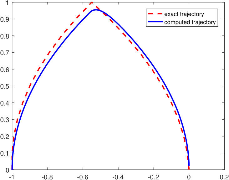 Figure 11
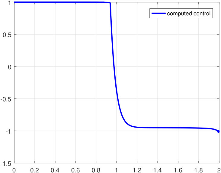 Figure 12
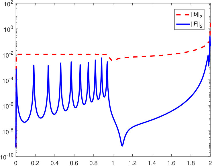 Figure 13
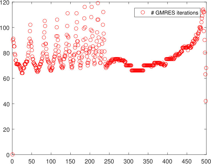 Figure 14
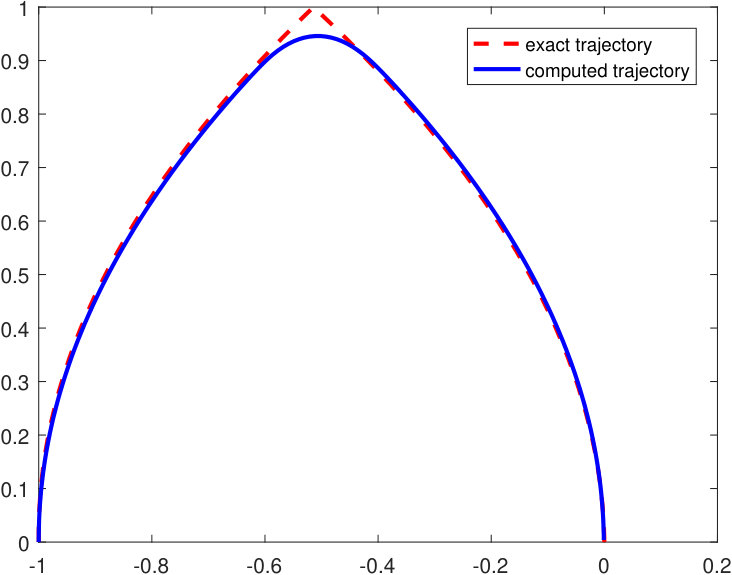 Figure 21
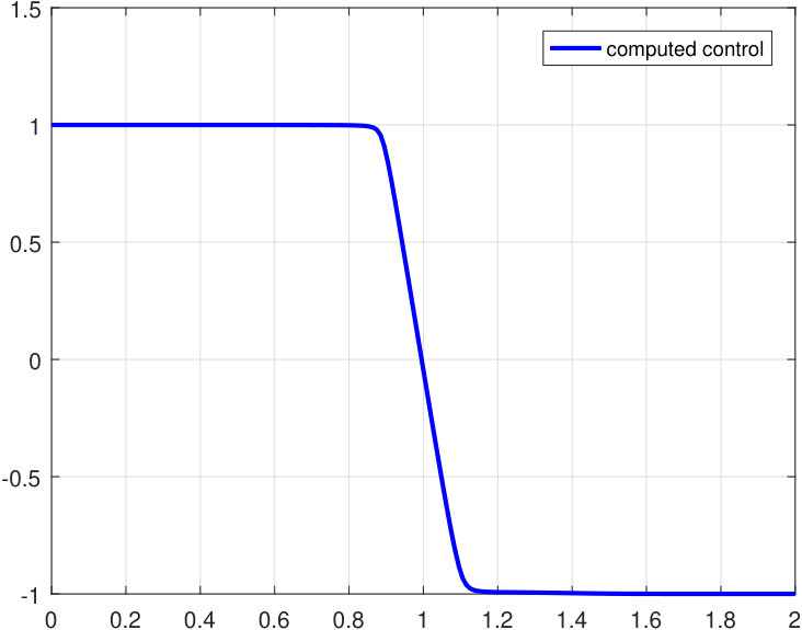 Figure 22
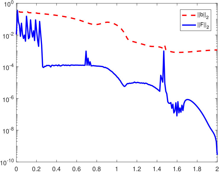 Figure 23
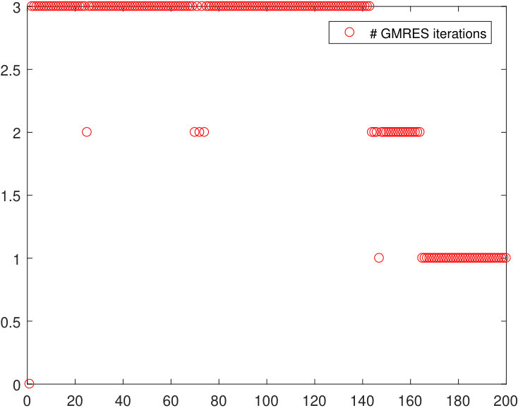 Figure 24
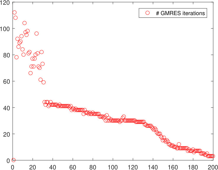 Figure 25
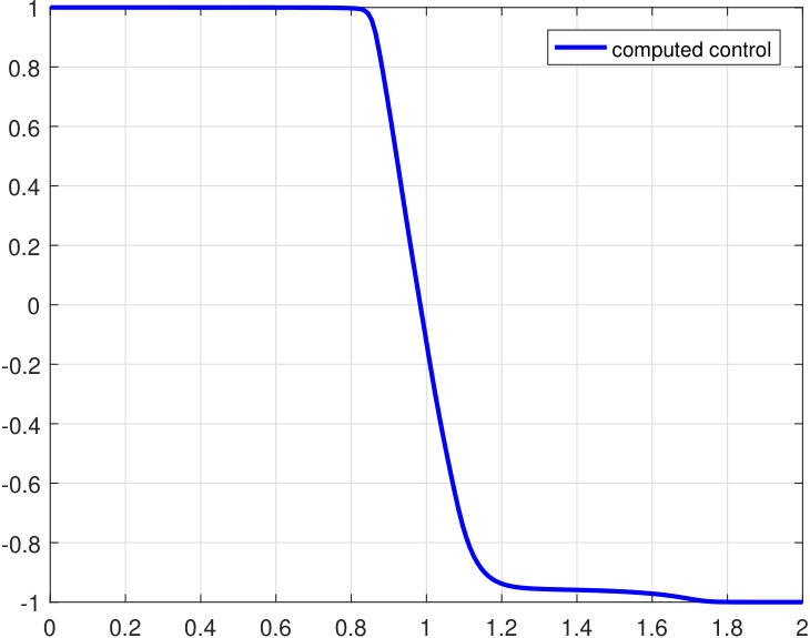 Figure 32
Peer Reviews
No public reviews on file for this paper yet. If you reviewed it on a platform where reviews are public (OpenReview, ICLR, NeurIPS, ICML), you can paste yours below so the community can read it here.
Videos
No videos yet. Explain this paper in a talk, walkthrough, or lecture? Add one.
Preconditioned warm-started Newton-Krylov methods for MPC with
discontinuous control††thanks: [email protected], [email protected]
Andrew Knyazev Mitsubishi Electric Research Laboratories (MERL) 201 Broadway, 8th floor, Cambridge, MA 02139, USA
Alexander Malyshev University of Bergen, Department of Mathematics, Postbox 7803, 5020 Bergen, Norway
Abstract
We present Newton-Krylov methods for efficient numerical solution of optimal control problems arising in model predictive control, where the optimal control is discontinuous. As in our earlier work, preconditioned GMRES practically results in an optimal complexity, where is a discrete horizon length. Effects of a warm-start, shifting along the predictive horizon, are numerically investigated. The method is tested on a classical double integrator example of a minimum-time problem with a known bang-bang optimal control.
1 Introduction.
We present and study numerically an approach to solution of minimum-time problems by the Model Predictive Control (MPC) method. The approach has been designed in our previous papers [9]-[13]. We apply it here to the double integrator problem, which is a classical example of the minimum-time optimal control problem. One of the main difficulties for numerical solution of this problem is caused by that the optimal control input is a function with large discontinuities, which makes the continuation procedures along the trajectories harder for accurate computation.
The minimum-time optimal control problems have been well studied; see e.g., [1, 2, 3, 6, 28]. In simple cases such as a double integrator with constraints on the control input [15], a closed-form of the feedback law can be found analytically. In general cases, obtaining a closed-form solution is a challenging task and a minimum-time open-loop trajectory is generated numerically by applying either direct methods, such as the direct shooting method, penalty function method, and SQP, or indirect methods such as the multiple shooting method and collocation method [4, 7, 14, 17, 18, 20],[23]-[27],[29]. To provide robustness to unmeasured uncertainties, the open-loop control can be augmented with a feedback stabilizer to the computed open-loop trajectory.
Applying the MPC philosophy to the minimum-time control involves recomputing the open-loop state and control trajectory subject to pointwise-in-time state and control constraints, terminal state constraint, and the current state as the initial conditions. The computed control trajectory is applied at the next time step; see, e.g., [16, 21, 30].
We use a time scaling linear transformation to obtain a fixed-end time problem, with the terminal time appearing as a multiplicative parameter in the dynamic equations. We then convert the model to a discrete time and formulate a prediction problem, where both the control input sequence and the horizon length, now appearing as a parameter, have to be optimized.
We use the continuation method for advancing the predictive horizon in time. Since the optimal control input is a piecewise continuous function and the discontinuities are severe, the perturbations of the unknown vectors during the continuation can be sufficiently large. There are two simple remedies for minimizing these perturbations: (1) application of the Newton-like iterations several times and (2) the use of suitable interpolations for current data when reusing them as a warm-start in the next horizon interval. In our numerical experiments, satisfactory results are obtained by the aid of both techniques. In some situations, the linear interpolation shows impressive improvements, in other situations, multiple application of the Newton-like iterations is the only tool for computations without failure.
In [13], we propose a new preconditioner technique for the Newton-like iterations. It works in the case, when the problem has only few state constraints, e.g., terminal state constraints. The double integrator problem satisfies these restrictions, and we present a construction of such preconditioner for this problem. The preconditioned iterations have the arithmetical cost , where is the number of grid points in the predictive horizon.
2 Formulation of the prediction problem
We want to develop a numerical method for solving the double integrator problem [2], where a bounded control input drives the dynamic system from an initial state to a final state in minimum time . We introduce the state variables , and convert the problem with the free terminal time to a problem with a fixed terminal time by the linear time scaling such that . The system dynamics after scaling becomes \frac{d}{d\tau}\left[\begin{array}[]{c}x_{1}\\ x_{2}\end{array}\right]=(t_{f}-t_{0})\left[\begin{array}[]{c}x_{2}\\ u\end{array}\right]. We also replace the inequality by the equality constraint , , where is a dummy (or slack) argument. Our goal is to minimize the performance index by choosing a suitable control input .
A general continuous-time model for the minimum time problem after time scaling reads as follows: given a performance index , find subject to the equality constraints
[TABLE]
where and are the state and control input, respectively. The vector function determines equality constraints, where possible dummy arguments correspond to inequality constraints. For instance, an inequality constraint can be replaced by the equality constraint or by , and then a suitable penalty term, e.g., must be added to the performance index , where is a small constant required by the interior point method [29].
Let us consider a discretization of the continuous-time model on the uniform grid , where . The adjustable variables are the control time sequence , , …, and the parameter that need to be simultaneously optimized. The discrete-time optimal control problem can be recast in the following form: given a performance index
[TABLE]
find
[TABLE]
subject to a fixed initial value and the equality constraints
[TABLE]
[TABLE]
[TABLE]
From several choices for the functions , and in the double integrator problem. we have tried two: (1) , , , and (2) , for a small and large .
To solve the discrete-time optimal control problem by the classical Lagrange multiplier method, we introduce the costate for the dynamics equations, the Lagrange multiplier for the equality constraints, and Lagrange multiplier for the terminal constraint and derive necessary optimality conditions are by means of the discrete Lagrangian
[TABLE]
where
[TABLE]
and
[TABLE]
The optimality conditions are given by the stationarity conditions
[TABLE]
Further derivations use the Hamiltonian function
[TABLE]
The optimality conditions are reformulated below as a system of nonlinear equations
[TABLE]
with respect to the unknown vector . We recall that in the MPC method denotes the current measured state vector, which serves as the initial value in the prediction problem, and is the current system time. The vector function is obtained from the optimality conditions after elimination of all states and costates by the following procedure.
Having the current measured state , set and compute , , by the forward recursion
[TABLE]
Then starting with the value
[TABLE]
compute the costate , , by the backward recursion
[TABLE] 2. 2.
Using the values and , , computed by the forward and backward recursions, compute the vector function as the vector . Explicit formulas for the components of can be found in [13].
3 The Newton-Krylov method
The system of nonlinear equations (2.1) with respect to must be solved in real time at each instance of the discrete system time. Assume that is an approximation to the exact solution . Then . Let us denote and . For a sufficiently small scalar , e.g. , which may be different from the system time step and from the horizon time step , we introduce the finite difference operator
[TABLE]
Equation (2.1) is then equivalent to the operator equation
[TABLE]
We suppose that is sufficiently small such that the operator is almost linear in the sense that with a tiny constant . Thus, solution of (2.1) is reduced to solving the operator equation
[TABLE]
for a given approximation and setting .
Given formulas for computing the vector function , we want to solver equation (2.1) at the points of the uniform grid , by using the above proposed approach.
At the initial state , we find an approximate solution to the equation by a suitable optimization procedure. The dimension of the vector is denoted by . Since
[TABLE]
the first block entry of , formed from the first elements of , is taken as the control at the state . The next state is either measured by a sensor or computed by the formula .
The computation of for is as follows. By , we denote the -th column of the identity matrix, where is the dimension of the vector . At time , we arrive with the state and the vector . The vector serves as the approximation , and such an approximation is often called the warm start. The difference operator
[TABLE]
implicitly determines an matrix with the columns
[TABLE]
which approximates the symmetric Jacobian matrix so that . At the current time , our goal is to solve the equation
[TABLE]
Then we set and choose the first components of as the control . The next state either comes from a sensor, estimated, or computed by the formula .
Equation (3.2) can be solved approximately by generating the matrix and then solving the system of linear equations using a direct method, e.g., the Gaussian elimination.
An alternative method of solving (3.2) is by a Krylov subspace iteration, e.g., by GMRES method [22], for which we do not generate the matrix explicitly. Namely, we simply use the operator instead of computing the matrix-vector product , for arbitrary vectors ; cf., [8]. The arithmetic cost of the alternative method can be often less than that of the direct method because the matrix is not generated and the cost due to the Gaussian elimination is avoided.
We refer to the Newton-like refinement by solving equation (3.2) with the GMRES method as the Newton-Krylov method.
Remark 1.
The above numerical procedure uses the so-called warm start. Specifically, the operator and the right-hand-side are computed at time using the value from the previous time as an approximation . This approximation does not take advantage of the structure of the underlying problem. In our case, the vector contains the components , , , , and computed in the prediction horizon . It is possible to apply, e.g., the linear interpolation of the variables , , from the previous horizon interval to the current horizon interval , where equals from and . Such an interpolation is referred to as the shifting along the predictive horizon; see a related discussion in [4].
Remark 2.
The shifting along the predictive horizon, described in Remark 1, is a light improvement, which may help in some situations. A more cardinal improvement of the warm start is solving the operator equation and subsequent correction several times, say, 2-3 Newton-like iterations instead of one.
4 Sparse preconditioner
Convergence of the GMRES iteration can be rather slow if the matrix is ill-conditioned. However, the convergence can be improved by preconditioning; see e.g. [22]. A matrix that approximates a matrix and such that computing the product for an arbitrary vector is relatively easy, is referred to as a preconditioner. The preconditioning for the system of linear equations formally replaces the original system with the equivalent preconditioned linear system . If the condition number of the matrix is small, convergence of iterative solvers for the preconditioned system become fast. Instead of , its inverse is often called a preconditioner.
Our specific optimization problem over a predictive horizon admits construction of efficient preconditioners with a sparse structure. These preconditioners have been introduced in [13], and we refer to this paper for a more detailed description.
The construction of is based on several observations. The first one is the fact that the Jacobi matrix is the Schur complement of the Jacobi matrix for the Lagrangian . If we denote the result of the forward and backward recursions by , then most entries of are approximated by the matrix due to the second fact, which affirms that the states , computed by the forward recursion, and the costates , computed by the subsequent backward recursion, satisfy the following property: , , and . The second fact is a corollary of theorems about the derivatives of solutions of ordinary differential equations with respect to a parameter; see, e.g., [19, 5]. The matrix is very sparse and easily computable. We have to generate explicitly by the formula only the last columns and rows of , where the integer denotes the sum of dimensions of and .
As a result, the setup of , computation of its LU factorization, and application of the preconditioner all cost floating point operations. The memory requirements are also of order .
5 Simulations of a Double Integrator System
To evaluate the effectiveness of the Newton-Krylov method, we compute a solution to the double integrator system with control input constraints: subject to , , , , , . We consider two discrete-time models of this problem and solve both numerically by the MPC approach, where the predictive horizon is the interval , being the current system time.
Model 1 of the predictive problem on the scaled horizon has the form
[TABLE]
subject to
[TABLE]
[TABLE]
[TABLE]
Model 2 of the predictive problem on the scaled horizon has the form
[TABLE]
subject to
[TABLE]
[TABLE]
[TABLE]
We choose and in Model 2. The initial state is , , and the terminal state is , in both models. The interior point penalty parameter and is fixed as suggested, e.g., in paper [29].
Below we give detailed formulas for an implementation of Model 1. Similar formulas can be easily derived for Model 2.
The components of the discretized problem on the predictive scaled horizon are as follows:
- •
, ;
- •
the unknown variables are the state \left[\begin{array}[]{c}x_{i}\\ y_{i}\end{array}\right], the costate \left[\begin{array}[]{c}\lambda_{1,i}\\ \lambda_{2,i}\end{array}\right], the control , the dummy variable , the Lagrange multipliers and \left[\begin{array}[]{c}\nu_{1}\\ \nu_{2}\end{array}\right], the parameter ;
- •
the state is determined by the forward recursion
[TABLE]
where ;
- •
the costate is determined by the backward recursion (, )
[TABLE]
where ;
- •
the system of equations , where
[TABLE]
has the following rows from the top to bottom:
[TABLE]
[TABLE]
[TABLE]
The sparse preconditioner is a symmetric matrix with the sparsity structure
[TABLE]
where is a block diagonal matrix with the nonsingular diagonal -blocks, ,
[TABLE]
The matrix block \left[\begin{array}[]{c}M_{12}\\ M_{22}\end{array}\right] consists of 3 columns and is computed by means of the operator as
[TABLE]
where are the columns , and of the unit matrix of order . The block is transpose to , .
The LU factorization of can be computed with floating point operations, e.g., as
[TABLE]
where . The setup and application of the preconditioner also cost operations.
6 Numerical results
All the plots are computed by the GMRES method with the absolute tolerance .
Figures 1, 2, 3, 4 show the numerical results for Model 1, where the horizon length equals 20. The exact and computed time to destination is . The system time between and is uniformly partitioned into 500 subintervals with the time step . Our MATLAB implementation fails when only 1 Newton’s refinement is used at each time instance , and it works with 2 Newton’s refinements per step. The failure is not cured by the shifting along the predictive horizon described in Remark 1. When the interval is partitioned into 1000 subintervals, our MATLAB program works with 1 Newton’s refinement at each step .
Figure 3 shows the Euclidean norm of the residual denoted by and the Euclidean norm of the residual after all Newton’s refinemens at time (2 refinements in Figure 3).
Figure 4 displays the total number of GMRES iterations at each time when the GMRES method is applied without preconditioner. The average number of GMRES iterations per step is about 77. The GMRES method with preconditioning uses only 2 iterations per step thus demonstrating more than the 35x speedup. We recall that our preconditioning provides the complexity of the prediction problem.
The interpolation by shifting along the predictive horizon from Remark 1 does not give an essential improvement in accuracy for Model 1 with the chosen time steps in the horizon and the system time. The multiple application of Newton’s refinements, however, provides an essential improvement in accuracy and computation without failure.
Figures 5–9 show the numerical results for Model 2. Again, the computed time to destination equals , but the system time between and is partitioned into 200 subintervals. The predictive horizon has the length . Our MATLAB program succeeds in computing the control input and trajectory with only 1 Newton’s refinement per step by using the shifting along the predictive horizon. The program fails without the shifting interpolation. The number of GMRES iterations without preconditioning is shown in Fig. 9 and its average value per step is about 35. The number of GMRES iterations with preconditioning shown in Fig. 8 is about 2.5 per step. Hence the speedup is about 14x.
We have run our program for Model 2, when , the time interval is partitioned into 200 subintervals, and only 1 Newton’s refinement is used. The program fails to compute without the shifting interpolation and works with the interpolation. Figure 10 displays the computed control input.
Models 1 and 2 demonstrate different behavior in our numerical experiments. Model 2 produces the control input with a smoother approximation of the discontinuity than Model 1 in spite of that its predictive horizon contains 70 grid points against 20 grid points in Model 1. Model 1 requires application of several Newton’s iterations per time step and the shifting interpolation is not enough for the work without failure. Model 2 works perfectly with the shifting interpolation and fails with it. The multiple Newton refinements help for Model 2 but the number of required refinements is not small. Thus, Model 1 with the chosen set of parameters requires multiple Newton iterations, and Model 2 with its own set of parameters requires the shifting interpolation along the horizon.
7 Conclusion
Our numerical experiments demonstrate that the Newton-Krylov method successfully works even in the cases, when the control input is discontinuous. Both the multiple Newton refinement and the interpolation by shifting along the predictive horizon can essentially improve accuracy of the computed solution and avoid failure during computations. The sparse preconditioner gives very good acceleration, e.g., a speedup about 15-30 times. A future research may include more advanced numerical examples and deeper study of the interpolation by shifting along the predictive horizon.
Acknowledgements.
We are very grateful to Ilya Lashuk for his guidance and help in using Model 2.
The reference list from the paper itself. Each links out to its DOI / PubMed record.
- 1[1] M. Athans and P. Falb, Optimal control: an introduction to the theory and its applications , Dover Publ., 2006.
- 2[2] A. E. Bryson, Jr. and Yu-Chi Ho, Applied optimal control: optimization, estimation, and control , Taylor & Francis, 1975.
- 3[3] D. Chen, L. Bako and S. Lecoeuche, The minimum-time problem for discrete-time linear systems: a non-smooth optimization approach , IEEE Int. Conf. Control Appl. (CCA), Dubrovnik, Croatia, pp. 196–201, 2012.
- 4[4] M. Diehl, H. J. Ferreau, and N. Haverbeke, Efficient numerical methods for nonlinear MPC and moving horizon estimation , in L. Magni et al. (eds.) Nonlinear Model Predictive Control, LNCIS 384, pp. 391–417, Springer, Heidelberg, 2009.
- 5[5] A. F. Filippov, Differential equations with discontinuous righthand sides , Springer Netherlands, 1988.
- 6[6] Z. Gao, On discrete time optimal control: a closed-form solution , in Proc. American Control Conf., pp. 52–58, Boston, MA, 2004.
- 7[7] P. Giselsson, Optimal preconditioning and iteration complexity bounds for gradient-based optimization in model predictive control , in Proc. American Control Conf., pp. 358–364, Washington D.C., USA, 2013.
- 8[8] C. T. Kelly, Iterative methods for linear and nonlinear equations , SIAM, Philadelphia, PA, 1995.