Renormalization Analysis for Degenerate Ground States
David Hasler, Markus Lange

TL;DR
This paper analyzes how the ground state properties of a finite quantum system with degeneracies change analytically with coupling strength, using operator renormalization techniques under mild infrared conditions.
Contribution
It extends operator theoretic renormalization methods to handle degenerate ground states in quantum systems coupled to relativistic bosons.
Findings
Ground state projection and energy are analytic functions of coupling constant.
Analyticity holds under mild infrared assumptions.
Operator renormalization is successfully extended to degenerate cases.
Abstract
We consider a Hamilton operator which describes a finite dimensional quantum mechanical system with degenerate eigenvalues coupled to a field of relativistic bosons. We show that the ground state projection and the ground state energy are analytic functions of the coupling constant in a cone with apex at the origin, provided a mild infrared assumption holds. To show the result operator theoretic renormalization is used and extended to degenerate situations.
Click any figure to enlarge with its caption.
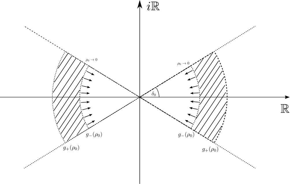 Figure 1
Peer Reviews
No public reviews on file for this paper yet. If you reviewed it on a platform where reviews are public (OpenReview, ICLR, NeurIPS, ICML), you can paste yours below so the community can read it here.
Videos
No videos yet. Explain this paper in a talk, walkthrough, or lecture? Add one.
Renormalization Analysis for Degenerate Ground States
David Hasler and Markus Lange
Department of Mathematics, Friedrich Schiller University Jena
Jena, Germany
Abstract
We consider a Hamilton operator which describes a finite dimensional quantum mechanical system with degenerate eigenvalues coupled to a field of relativistic bosons. We show that the ground state projection and the ground state energy are analytic functions of the coupling constant in a cone with apex at the origin, provided a mild infrared assumption holds. To show the result operator theoretic renormalization is used and extended to degenerate situations.
1 Introduction
Models of quantum field theory which describe low energy phenomena of quantum mechanical matter interacting with a quantized field of massless particles have been mathematically intensively investigated (see for example [27] and references therein, for an early work see [14]). These models are used to study non relativistic matter interacting with the quantized radiation field or electrons in a solid interacting with a field of phonons. Physical properties such as existence of ground states, dispersion relations, and resonances have been treated mathematically rigorous. In particular, the method of operator theoretic renormalization, introduced by Bach Fröhlich and Sigal [7, 8], has been used in the literature to study ground states and resonances [3, 16, 25, 22, 20, 21, 13, 12, 4, 11]. However, the application of operator theoretic renormalization usually requires that the unperturbed eigenstate is non degenerate or at least protected by a symmetry. In this paper we extend operator theoretic renormalization to situations where the unperturbed eigenvalue is degenerate and the degeneracy is lifted after the interaction is turned on. We note that degenerate situations do occur in physically realistic models, see for example [1]. To keep notation simple we treat the ground state. Resonances can be treated by the same ideas as used in this paper with additional notational complexity. This is planned to be addressed in a forthcoming paper.
More precisely, we consider a quantum mechanical atomic system described by a Hamilton operator acting on a so called atomic Hilbert space. For simplicity we assume that the atomic Hilbert space is finite dimensional (we expect that this assumption is not essential and can be relaxed in a straight forward way). Furthermore, we assume that the atomic system interacts with a quantized field of massless bosons by means of a linear coupling. The resulting Hamiltonian describing the total system is also referred to as generalized spin boson Hamiltonian. We assume that the interaction satisfies a mild infrared condition. The infrared condition is needed for the renormalization analysis to converge. It can be shown to include realistic models of non relativistic quantum electrodynamics by means of a so called generalized Pauli Fierz transformation [25]. We assume that the Hamiltonian of the atomic subsystem has a degenerate ground state, which is lifted by formal second order perturbation theory in the coupling constant (first order perturbation theory does not affect the ground state energy for models which we consider). We show that the ground state exists for small values of the coupling constant, a result already known in the literature [15, 17, 23, 26]. Furthermore, we show that the ground state projection as well as the ground state energy are analytic as a function of the coupling constant in an open cone with apex at the origin. This result is new and it is in contrast to non degenerate situations, where it has been shown that the ground state projection and the ground state energy are analytic functions of the coupling constant [16]. We do not assume that this is an artefact of our proof. In fact, we conjecture that in the degenerate case there may be situations in which the ground state projection and possibly the ground state energy are not analytic in a neighborhood of zero. In a related model, where a hydrogen atom is minimally coupled to the quantized electromagnetic field, non analyticity in the fine structure constant has been shown [9].
Although we do not obtain analyticity in a neighborhood of zero, analyticity in a cone is of interest in its own right. It is for example a necessary ingredient to show Borel summability. Borel summability methods allow to recover a function from its asymptotic expansion. An asymptotic expansion may for example be obtained using the techniques employed in [2, 10, 18, 6, 5].
In the following section we state the model and the main result. The subsequent sections are devoted to the proof of the main result.
2 Model and Statement of Results
We consider the following model. Let the atomic Hilbert space be modeled by
[TABLE]
and equipped with the standard scalar product. Furthermore we equip with the operator norm, which we denote by . Let the Fock space
[TABLE]
with model the quantized radiation field. We denote the Fock vacuum by and the Hilbert space of the total system by
[TABLE]
We assume that is self adjoint. To simplify our notation we define for
[TABLE]
and denote by and the usual creation and annihilation operator satisfying canonical commutation relations. For formal definitions of the annihilation and creation operator and associated field operators we refer the reader to B. For we define
[TABLE]
which are densely defined closed linear operators in the Hilbert space. We define the free field operator by
[TABLE]
which is defined in the sense of forms. For we shall study the following operator
[TABLE]
where the so called interaction is given by
[TABLE]
We note that is infinitesimally bounded with respect to if . Let denote the ground state of , and let denote the projection onto the eigenspace of with eigenvalue , and let . Define
[TABLE]
which is a selfadjoint mapping on the ground state space of . For we denote the open disk in the complex plane by
[TABLE]
In order for the renormalization analysis to be applicable we shall need an infrared condition. For this we define for
[TABLE]
where we defined
[TABLE]
Theorem 2.1**.**
Let . Suppose and let be given by (2.3). Let denote the smallest eigenvalue of . Assume that is simple. Let , and let
[TABLE]
Then there exists a such that for all the operator has an eigenvector and an eigenvalue such that
[TABLE]
The eigenvalue and eigenprojection are continuous on and analytic in the interior of . Furthermore for real the number is the infimum of the spectrum of .
Remark 2.2**.**
Let denote the projection onto the vacuum vector . We note that
[TABLE]
which is exactly the second order energy correction in formal perturbation theory. **
Remark 2.3**.**
If is the number operator we have the symmetry . This implies that eigenvalues do not depend on the sign of . And if they happen to have an asymptotic expansion it cannot depend on odd powers of .**
Remark 2.4**.**
Generically one can assume that either a degeneracy of an eigenvalue remains after the interaction is added (which happens if the degeneracy is protected by a symmetry, e.g., spin degeneracy) or it is lifted at some finite order. In this paper we assume that the degeneracy of the ground state is lifted at second order. We believe that the methods used in this paper are also usefull to treat degeneracies which are lifted at higher than second order, by possibly inserting several initital Feshbach maps, with energy cutoffs depending on the coupling constant. **
Remark 2.5**.**
Borel summability methods allow in certain situations to recover a function from its asymptotic expansion, provided it satisfies a strong asymptotic condition. Theorem 2.1 together with Remark 2.3 can be used to show that the ground state energy as a function of satisfies the analyticity requirement of a strong asymptotic condition [24]. Suppose and are as in Theorem 2.1. Define the function with and . Then is analytic in the interior of the cone and extends continuously onto the boundary. Moreover satisfies the analyticity requirement for a strong asymptotic condition. Now suppose there were and such that
[TABLE]
for all and all . Then could be recovered uniquely by the method of Borel summability, see [24, Watson’s theorem]. **
The remaining part of the paper is devoted to the proof of Theorem 2.1. First we give an overview of the proof, before we comment on the organization of the paper. As already mentioned in the introduction, the proof is based on an operator theoretic renormalization analysis. Such an analysis is based on the so called smooth Feshbach map and its isospectrality properties. Let us introduce the relevant definitions and properties. For additional details we refer the reader to [3, 16].
Suppose and are commuting, nonzero bounded operators, acting on a separable Hilbert space and satisfying . We shall refer to and as smoothed projections. By a Feshbach pair for we mean a pair of closed operators in with the same domain such that the following properties hold:
- (i)
and commute with ,
- (ii)
, are bijections with bounded inverse.
- (iii)
is a bounded operator.
Given a Feshbach pair for , we call the operator
[TABLE]
the Feshbach operator. The mapping is called Feshbach map. Central for our proof is the isospectrality property of the Feshbach map, stated in the following theorem. To formulate it one introduces the so called auxiliary operator
[TABLE]
Theorem 2.6** ([16]).**
Let be a Feshbach pair for on a separable Hilbert space . Then
[TABLE]
are linear isomorphisms and inverse to each other.
The renormalization analysis is based on a carefully designed iterated application of the smooth Feshbach map. Before one can start this machinery, we need to control the degeneracy. For this, we perform two so called initial Feshbach maps. The first Feshbach map uses a smoothed projection given as a tensor product. The first factor acts on the atomic Hilbert space and projects orthogonally onto , the degenerate ground state eigenspace of the atomic Hamiltonian. The second factor acts on Fock space and is given by a smooth cutoff function of the free field energy, such that its range is contained in a spectral subspace of field energies between zero and . The second Feshbach map uses a smoothed projection given again as a tensor product. The first factor now projects onto the subspace of belonging to the lowest energy eigenvalue of . The second factor is given again by a smooth cutoff function of the free field energy, with range contained in a spectral subspace of even smaller field energies between zero and . This procedure will resolve the degeneracy and hence allows us to initiate the usual renormalization analysis in Fock space as introduced in [3].
In the proof we will choose larger than but smaller than . More precisely, we will show the following. For any there exists a and positive numbers with , uniformly in the model parameters, such that for all coupling constants in a sectorial region of the complex plane with
[TABLE]
both Feshbach maps are isospectral and respect necessary Banach space estimates needed for operator theoretic renormalization to be applicable, see Figure 1. Then for in a sectorial region of an annulus we shall obtain analyticity of the ground state projection and ground state energy by invoking an analyticity result of Griesemer and Hasler [16]. Moreover, we show that we can choose such that as (at the same time but this is no problem as long as ). Hence the analyticity in a cone with apex at the origin will follow as tends to zero.
The remaining part of the paper is organized as follows. In Section 3 we define the first Feshbach map with parameter and prove the Feshbach pair criterion, which establishes isospectrality. In Section 4 we define Banach spaces of matrix valued integral kernels. These Banach spaces parametrize subspaces of operators in Fock space and allow to control the flow of the operator theoretic renormalization analysis. Thereby we extend the Banach spaces of integral kernels introduced in [4] to include matrix valued integral kernels, in order to adapt degenerate situations. In Section 5 we introduce polydiscs around the free field energy in a subspace parametrized by a Banach space of integral kernels, (5.2). We then show in Theorem 5.1 that the first Feshbach operator lies in such a polydisc, where the radii of the polydisc can be made arbitrarily small for sufficiently small . In Section 6 we define the second Feshbach map with parameter , which will be responsible for lifting the degeneracy. We establish necessary estimates, which will be used to show the Feshbach pair criterion for the second step. We note that for these estimates, in particular Lemma 6.3, we need the coupling constant to lie in a cone. We conclude the section with an abstract Feshbach pair criterion. In Section 7 we prove an abstract Banach space estimate for the second Feshbach step, which will be used to show that the second Feshbach operator lies in a suitable polydisc around the free field energy. Section 8 is devoted to the proof of the main result Theorem 2.1. Having the abstract results of the previous two sections at hand, we will finally choose as a function of , such that the second Feshbach map satisfies indeed the Feshbach pair criterion, establishing isospectrality, and such that the second Feshbach operator lies in a suitable polydisc, allowing the application of the analyticity result [16]. In particular, we rigorously justify (see (8.4)) the situation outlined in Figure 1 together with (2.11).
3 Initial Feshbach Step
Without loss we assume that the distance of from the rest of the spectrum of is , i.e.,
[TABLE]
This can always be achieved by a suitable scaling. In this section we define the initial Feshbach operator. For definitions and conventions we refer to [3, 16] and collect for the convenience of the reader basic notions in the appendix. We will show for in a neighborhood of and for sufficiently small, that and are a Feshbach pair for a generalized projection, which we will now introduce. We fix two functions and in satisfying the following properties:
- (i)
, if , and , if ,
- (ii)
.
For we define the following operator valued functions
[TABLE]
and we define by means of the spectral theorem the linear operators in
[TABLE]
It is easily verified that .
The following proposition provides us with conditions for which the initial Feshbach operator will be defined.
Theorem 3.1** (Feshbach Pair Criterion for 1st Iteration).**
Let , and . The operators and are a Feshbach pair for , if
[TABLE]
Furthermore one has the absolutely convergent expansion
[TABLE]
Let us now provide proof of Theorem 3.1. For this we shall make use of the following two lemmas.
Lemma 3.2**.**
Let . Then for we have
[TABLE]
Proof.
This follows from (A.2). For the annihilation operator we find for
[TABLE]
and likewise we estimate the corresponding expression involving a creation operator. ∎
Lemma 3.3**.**
Let and . The operator is invertible on the range of and we have the bound
[TABLE]
and for all the bound
[TABLE]
Proof.
First we show that is bounded invertible on the range of . It follows for a normalized that
[TABLE]
and it follows from (3.1) that for a normalized we have
[TABLE]
Thus from the above two inequalities it follows that is bounded invertible on the range of and that (3.4) holds. We estimate further,
[TABLE]
and if we set
[TABLE]
Now the above two inequalities show (3.5). ∎
Proof of Theorem 3.1. To prove the invertibility, we note that and leave the range of invariant and that is bounded invertible on the range of . We use Lemmas 3.3 and 3.2. We write
[TABLE]
and we use the following identity
[TABLE]
Thus the bounded invertibility follows from Neumanns theorem provided
[TABLE]
Now using Lemma 3.2, note that commutes with , and (3.5) of Lemma 3.3, we obtain
[TABLE]
Thus, if we choose , then the proposition follows. ∎
4 Banach Space of Integral Kernels
To control the renormalization transformation, in particular proving its convergence, we introduce the following Banach spaces of integral kernels. We note that the choice of these spaces is not unique. We choose the Banach spaces such that they are suitable for the model which we consider. Specifically, the Banach spaces which we introduce below are a straight forward generalization of the spaces defined in [3] or [16] to matrix valued integral kernels. A generalization to matrix valued integral kernels seems to be a canonical choice to accommodate degenerate situations.
For we define the Banach space as the space of continuously differentiable matrix valued functions
[TABLE]
with norm
[TABLE]
where stands for the derivative. Let . For a set we write
[TABLE]
where we recall the notation of Eq. (2.1). For we write
[TABLE]
[TABLE]
[TABLE]
Moreover, we shall use
[TABLE]
For with and let denote the space of measurable functions satisfying the following three properties.
- (i)
are symmetric with respect to all permutations of the arguments from and the arguments from , respectively;
- (ii)
for , we have , provided ;
- (iii)
The following norm is finite
[TABLE]
where
[TABLE]
Remark 4.1**.**
We note that is given as the subspace of
[TABLE]
consisting of elements satisfying Conditions (i) and (ii) above. Note that the norm is equivalent to the natural norm of (4.1) (given by the theory of Banach space valued -functions), which is the norm chosen in [16]. Moreover, we will identify (4.1) as a subspace of by means of
[TABLE]
Henceforth we shall use this identification without comment. Furthermore, we remark that
[TABLE]
with the natural convention that for the empty Cartesian product consists of a single point and that there is no integration in that case.**
For given and we define the Banach space
[TABLE]
with norm
[TABLE]
for .
Next we define a linear mapping , where and . For this we will use the notation
[TABLE]
If define . For and define the operator on
[TABLE]
The following lemma is proven in [3, Theorem 3.1]
Lemma 4.2**.**
Let and with . For we have
[TABLE]
Using our notation above and the convention that for it is trivial to extend this lemma to the case .
For sequences we define the operator as the sum
[TABLE]
where the sum converges in operator norm, which can be seen using (4.4).
A proof of the following theorem can be found in [3] with a modification explained in [19].
Theorem 4.3**.**
Let and . Then the map is injective and bounded. For and for with we have
[TABLE]
The renormalization transformation will involve a rescaling of the energy. This rescaling is described by means of a dilation operator, which we shall now define.
Definition 4.4**.**
Let . We define the operator of dilation on the one particle sector by
[TABLE]
where we use the notation We define the operator of dilation on Fockspace by
[TABLE]
We define the mapping called rescaling by dilation by
[TABLE]
Remark 4.5**.**
We note that that by definition Moreover, one can show that
[TABLE]
The following lemma relates the scaling transformation to a scaling transformation of the integral kernels. It is straight forward to verify by the substitution formula.
Lemma 4.6**.**
For define the scaling transformation of the integral kernel by
[TABLE]
Then
[TABLE]
Remark 4.7**.**
For one finds
[TABLE]
This illustrates that after a renormalization step, which will be introduced below, the relative size of the perturbative part , , will shrink compared to the unperturbed part . **
5 Banach Space Estimate for the first Step
In Section 3 we showed that the operators , are a Feshbach pair for , provided the coupling constant is in a sufficiently small neighborhood of zero and the spectral parameter is sufficiently close to the unperturbed ground state energy. In particular, if the assumptions of Theorem 3.1 hold, we can define the operator
[TABLE]
which we call the first Feshbach operator. The goal of this section is to show that the first Feshbach operator is close to the free field energy. The distance will be measured in terms of the norms introduced in the previous section. More precisely, we define the following polydiscs of the free field energy. For given we define by
[TABLE]
We shall denote the dimension of the space of ground states of by
[TABLE]
Moreover, we introduce the following global constant
[TABLE]
[TABLE]
which will be used in various estimates. For the renormalization analysis to be applicable, we need a stronger infrared condition, which is expressed in terms of the norm . We note that as a consequence of the definition we have
[TABLE]
This inequality shows that the criterion for the Feshbach pair property obtained in Section 3 can be expressed in terms of . We can now state the main theorem of this section.
Theorem 5.1** (Banach Space Estimate for 1st Feshbach Operator).**
Let , and . Then there exist constants , such that, if , and
[TABLE]
the pair of operators is a Feshbach pair for , and
[TABLE]
for
[TABLE]
Remark 5.2**.**
We note that the explicit form of the constants , , and can be read off from Inequalities (5.27)–(5.29). Only depends on . **
The remaining part of this section is devoted to the proof of Theorem 5.1. First observe that in view of (5.5) and (5.3) we see that assumption (5.6) implies the assumption (3.2) of Theorem 3.1 holds. Thus is a Feshbach pair for provided is in a neighborhood of zero and is in a neighborhood of the unperturbed ground state energy. Thus by Theorem 3.1 we can expand the resolvent in the Feshbach operator in a absolutely convergent Neumann series (3.3). We shall bring the resulting Neumann series into normal order by using the pull-through formula, see Lemma A.3, and applying a generalized version of Wicks theorem, see Theorem C.1. First we use an alternative notation for our original Hamiltonian and we define
[TABLE]
We set and use the notation
[TABLE]
We note that the expression is analogous to (4.3), apart from the fact that the domain of integration is different and there is no projection. To distinguish this difference we use a superscript zeroth order. In the new notation the interaction reads
[TABLE]
For the bookkeeping of the terms in the Neumann expansion we introduce the following multi-indices for
[TABLE]
Now inserting the alternative expression for the interaction, (5.9), into the convergent Neumann Series (3.3), and using the generalized Wick theorem, Theorem C.1, we obtain a sum of terms of the form
[TABLE]
where the definition of is given in (C.6), and where we used the definitions
[TABLE]
[TABLE]
We use the natural convention that there is no integration if and that the argument is dropped if . Note that the appearance of the ’s in the arguments on the r.h.s. of (5.10) is due to the scaling transformation in eq. (5.1). Thus we have shown the algebraic part of the following result.
Proposition 5.3**.**
Suppose the assumptions of Theorem 3.1 hold, i.e., let , and (3.2). Define
[TABLE]
and for with define
[TABLE]
Assume that the right hand sides converge with respect to the norm for some and . Then for the symmetrization we have
[TABLE]
Proof.
Let be defined as the integral kernel obtained by the right hand sides of (5.13) and (5.12), if we sum only up to . Then by the absolute convergence of the Neumann Series (3.3) and the application of the generalized Wick theorem, Theorem C.1, as discussed above, we find
[TABLE]
A detailed description how to obtain the integral kernels is given in Appendix A of [16], see also [3]. The assumption that the right hand sides of (5.13) and (5.12) converge with respect to the norm imply in view of Theorem 4.3 that
[TABLE]
Our next goal is to show Inequalities (5.27), (5.28), and (5.29), below. These estimates will on the one hand imply that right hand sides of (5.13) and (5.12) converge with respect to the norm , and on the other hand establish a proof of Theorem 5.1. To obtain the desired estimates we will use the bounds, collected in the following lemma.
Proposition 5.4**.**
For all , , , , and we have
[TABLE]
and
[TABLE]
where .
Remark 5.5**.**
We note that in contrast to Eq. (7.5) in Lemma 7.3 (see also [3] Lemma 3.10) we have an additional factor , which yields an improved estimate. The proof of of Theorem 5.1, which we present, will need this improved estimate.**
To show the above proposition we will use the estimates from the following lemma.
Lemma 5.6**.**
For let .
- (a)
Let . Then for all , with , all , and
[TABLE]
[TABLE]
[TABLE]
- (b)
For all , and we have
[TABLE]
Proof.
Eq. (5.17) follows from the proof of Lemma 3.2. Eqns. (5.18) and (5.19) follow also from the proof of Lemma 3.2 and (A.1). Estimate (5.20) follows from Lemma 3.3. To show Estimate (5.21) we calculate the derivative
[TABLE]
To estimate the terms on the right hand side we use again Lemma 3.3 together with
[TABLE]
Proof of Proposition 5.4. Let . We estimate using
[TABLE]
where denotes the operator norm, and Inequalities (5.17)–(5.21). First we have for
[TABLE]
To calculate the derivative we use Leibniz rule and we obtain similarly using again equation (5.23) and Inequalities (5.17)–(5.21). We find for
[TABLE]
Now we can estimate inserting (5.24) and (5.25), respectively,
[TABLE]
[TABLE]
Adding above estimates yields (5.14). Eqns. (5.15) and (5.16) follow similarly noting that and can only occur if is even and on the very left we have a annihilation operator and on the very right a creation operator. ∎
Proof of Theorem 5.1. It suffices to establish inequalities (5.27)–(5.29), below. Let denote the set of tuples with , , and
[TABLE]
Such tuples obviously satisfy . Using this identity, we now estimate the norm of (5.13) using (5.14) and (5.5). This yields
[TABLE]
where in the last inequality we estimated the summands , separately and summed over the terms with , as we now outline. First we note that (5.26) implies that is empty unless , and that the number of elements with is bounded above by . Specifically for , we have only two terms: equal or equal . For we use that implies . For we use . These considerations establish (5.27). We now estimate the norm of (5.12) using (5.16), by means of a similar but simpler estimate
[TABLE]
Analogously we have using (5.15)
[TABLE]
The series on the right hand sides in (5.27)–(5.29) converge if (5.6) holds. Thus Theorem 5.1 now follows in view of equations (5.27)–(5.29). ∎
6 Second Feshbach Step
In this section we perform our second Feshbach step. We want to note that the field energy cutoff of the first Feshbach step will be henceforth denoted by while the field energy cutoff of the second Feshbach step will be denoted by . First we approximate , which is the content of the following lemma. We recall the mapping , which was defined in (2.5), and that its ground state energy, , is by assumption a simple eigenvalue.
Lemma 6.1** (Free Approx. to 1st Feshbach).**
There exists a constant such that the following holds. Let , , and suppose
[TABLE]
If , then the defining series of , i.e., the r.h.s. of (5.12), converges absolutely and
[TABLE]
Remark 6.2**.**
We note that if we replaced the in front of by one, then the proof given below would yield a bound only of order . **
Proof.
From (5.12) we see that
[TABLE]
From the definition (5.10) we see, that the summand with is only non-vanishing if and and that summands with odd vanish. Using this we can write
[TABLE]
where we introduced the notation
[TABLE]
The second term can be estimated similarly to (5.29), i.e., using (5.15) we find
[TABLE]
In order to obtain a suitable estimate for we use that has a natural decomposition into a sum of two terms and we calculate the vacuum expectation using the pull-through formula
[TABLE]
First we estimate the relative error if we replace by , that is we show for
[TABLE]
To estimate the first term in (6.4) we use common denominators
[TABLE]
This yields
[TABLE]
This explains the first contribution on the right hand side of (6.5). We estimate the second term in (6.4) similarly. For we write
[TABLE]
This yields
[TABLE]
This explains the second contribution on the right hand side of (6.5). Next we show that
[TABLE]
To estimate the first term in (6.4) with we use
[TABLE]
and make use of
[TABLE]
We estimate the second term in (6.4) with using for that
[TABLE]
This gives (6.8). Finally, inserting estimates of (6.3), (6.5), and (6.8) into (6.2) shows the lemma. ∎
Let denote the projection onto the one dimensional eigenspace of with eigenvalue and let . We mention that the superscript originates from the fact that these expressions are obtained by formal second order perturbation theory. For define
[TABLE]
and
[TABLE]
Recall that we assumed that the distance, , from the lowest to the second lowest eigenvalue of is one. By the assumption the following expression is positive
[TABLE]
which follows from an easy minimization problem, yielding
[TABLE]
Let . We shall assume the following inequalities
[TABLE]
and
[TABLE]
hold. Next we show the following lemma, which will establish the required invertibility.
Lemma 6.3** (Invertibility of Free Approx to 1st Feshbach).**
Suppose . Let satisfy (6.12) and (6.13). Then for we have
[TABLE]
Proof.
For notational simplicity we shall write
[TABLE]
For normalized in the range of we have
[TABLE]
where in the last inequality we used on the one hand that for we have by (6.11)
[TABLE]
and that on the other hand we used that for we have
[TABLE]
by (6.12). Using (6.13) in (6.15) it now follows that
[TABLE]
Next we consider for normalized in the range of
[TABLE]
where we used that on the one hand side we have for
[TABLE]
and on the other hand we have for
[TABLE]
by (6.12). Thus we can invert the operator on the range of . ∎
In order to perform a second Feshbach iteration, we choose the following decomposition
[TABLE]
where
[TABLE]
where
[TABLE]
Remark 6.4**.**
We note that decomposition (6.16) into free part and interacting part is not unique. The isospectrality property of the smooth Feshbach merely requires that the free part commutes with the smoothed projections. This issue is pointed out in Remark 2.4 in [3]. Alternatively, we could use the decomposition according to
[TABLE]
The proof given in this paper would carry through also with this decomposition, with only notational modifications. **
Thus we can now prove the main result of this section.
Theorem 6.5** (Abstract Feshbach Pair Criterion for 2nd Iteration).**
Assume that the smallest eigenvalue of is simple. Let . Suppose
[TABLE]
and . Then the operators and are a Feshbach pair for , provided
- (i)
* is invertible on the closure of and*
[TABLE]
- (ii)
the following inequality holds
[TABLE]
In this case we have the absolutely convergent expansion
[TABLE]
Proof.
First observe that commutes with . The Feshbach pair property follows from (i) and (ii) and Neumanns theorem. The second claim follows again by Neumanns theorem. ∎
Remark 6.6**.**
In the proof of the main theorem, in Section 8, we will determine an explicit relation among and and . Using this relation we will verify assumption (i) and (ii) of the above theorem by the help of Lemmas 6.1 and 6.3 . **
7 Banach Space Estimate for the second Step
Using estimates of the previous section we will show in Section 8 that is indeed a Feshbach pair for . For the moment we will assume that the Feshbach property is satisfied. In that case we can define
[TABLE]
provided the right sides exist. Similar to Section 5 we now want to show that there exists a sequence of integrals kernels such that
[TABLE]
This will follow as a conclusion of the following theorem.
For notational compactness we introduce in this section the following constant
[TABLE]
Theorem 7.1** (Abstract Banach Space Estimate for 2nd Feshbach Operator).**
Let and assume that the smallest eigenvalue of is simple. Let . Suppose
[TABLE]
and .
- (i)
* is invertible on the closure of and *
,
- (ii)
.
Then and are a Feshbach pair for . Moreover, suppose
[TABLE]
and
[TABLE]
Then
[TABLE]
where
[TABLE]
In order to prove Theorem 7.1 we first use the Neumann expansion given in (6.21) and we normal order the resulting expression using the generalized Wick Theorem, stated in the appendix. The result is given in Proposition 7.2 below, and can be obtained as in [3, Theorem 3.7]. To state it we recall the following notation
[TABLE]
for . We define
[TABLE]
For we defined
[TABLE]
where we use the natural convention that there is no integration if and that the argument is dropped if . Moreover we defined for the expressions and for we have set
[TABLE]
and is defined as in (C.6). We note that we used similar notation as in the previous section.
Proposition 7.2**.**
Define
[TABLE]
and for define
[TABLE]
Assume that the right hand side converges with respect to the norm . Let be the symmetrization w.r.t. and of . Then
[TABLE]
The proof of this proposition is analogous to the proof of Proposition 5.3. To prove Theorem 7.1, we shall need the estimate given in the following lemma.
Lemma 7.3**.**
Suppose the assumptions of Theorem 7.1 hold. For fixed and and we have
[TABLE]
with and the convention that for .
Remark 7.4**.**
We note that in contrast to [3] we do not have in (7.2) and (7.3) the conditions and , respectively. The proof of Lemma 7.3 is still similar to the proof of Lemma 3.10 in [3] however we have to take into account more terms. These terms are hidden in our notation, see Chapter 4.**
Proof of Lemma 7.3.
We start by estimating the resolvents. Let for . Then for and we have
[TABLE]
and for ,
[TABLE]
[TABLE]
where we used a similar equation as (5.22).
Now we estimate and using a variant of (5.23).
[TABLE]
Similarly we get with Leibniz’ rule
[TABLE]
To estimate the norm we shall use the following estimate
[TABLE]
where the first equality follows by the substitution formula for integrals, the second line follows from the estimate in Lemma 4.2, and the last line follows from Fubini’s theorem. Using (7.6) together with (7.8) we find
[TABLE]
Similarly using (7.7) together with (7.8) we find
[TABLE]
Adding Inequalities (7.9) and (7.10) establishes the estimate in (7.5). ∎
The proof of Theorem 7.1 is similar to the proof of Theorem 3.8. given in [3].
Proof of Theorem 7.1. The operators and are a Feshbach pair for by Theorem 6.5. First we use Lemma 7.3 to estimate (7.2). We shall write Since and , we have . Moreover, we use that . With this we find for
[TABLE]
Inserting this in we obtain the following bound
[TABLE]
where in the second last inequality we used a substitution of summation variables and in the last inequality we used that since . By the assumptions of the theorem we have
[TABLE]
Inserting this into (7) we find
[TABLE]
where we used that by assumption
[TABLE]
and moreover we used that for .
It remains to estimate (7.3). To this end we recall that for we see from Lemma 7.3 that
[TABLE]
Using this we find for the derivative
[TABLE]
where we used that by assumption
[TABLE]
Analogously we estimate
[TABLE]
provided (7.16) holds. The claim now follows from Equations (7), (7.15) and (7.17). ∎
8 Proof of the Main Theorem
Let denote the closed ball with radius .
Theorem 8.1** (Analyticity Theorem of Griesemer-Hasler [16]).**
*Let , and let be sufficiently small. Then for sufficiently small there exist positive constants , and such that the following holds.
Let be an open subset of and let be an analytic function. Let be an open subset of such that for all we have*
[TABLE]
Suppose is an valued analytic function on , such that for all
[TABLE]
Then there exist analytic functions and , nowhere vanishing, such that for all
[TABLE]
If furthermore on , then for real the operator has a bounded inverse for all .
The proof of this theorem follows directly from the proof of Theorem 1 in [16, pp. 610-611]. The only difference being that the theorem given above does not involve the initial Feshbach step and has therefore a shorter proof. In the application of Theorem 8.1, which we have in mind, the parameter in the theorem will be played by the coupling constant . Furthermore the energy cutoff will be an order one quantity, i.e., independent of the coupling constant. Now we are ready to prove the main result of this paper.
Proof of Theorem 2.1. Fix . Let and by chosen sufficiently small such that the assertion of Theorem 8.1 holds. The idea will be to choose energy cutoffs, and , at the first and second Feshbach step so that for in a sectorial region of an annulus, we can apply Theorem 8.1. As we let the outer and inner radius of the annulus tend to zero we will obtain the desired result.
[TABLE]
Choose and . For we define
[TABLE]
We shall assume that
[TABLE]
We consider the following sectorial region of an annulus, determined by the conditions and
[TABLE]
In view of the upper bound in (8.4), we conclude from Theorem 5.1 (Banach Space Estimate for 1st Feshbach Operator) that there exists a finite constant such that for satisfying (8.3) and all with (8.4) and we have
[TABLE]
Next we want to use Theorem 6.5 (Feshbach Pair Criterion for 2nd Iteration). Observe that by (8.3) the assumptions on the ’s and by (8.3) the assumptions (6.12) and (6.13) of Theorem 6.5 are satisfied for with (8.4). To apply the theorem we consider the decomposition defined in (6.16) where
[TABLE]
By Lemma 6.1 (Free Approx to 1st Feshbach) we see that for the difference to the free approximation (6.19) there is some constant such that
[TABLE]
where we used the upper bound in (8.4). By (8.2) we see that the right hand side of (8.6) is less than provided is sufficiently small. Thus by Neumann’s theorem and Lemma 6.3 we see that is invertible on and
[TABLE]
Furthermore, we see from (8.7) and (8.5) that
[TABLE]
We note that
[TABLE]
tends to zero for . In view of (4.6) we see that condition (6.20) of Theorem 6.5 is satisfied for small. Thus and are a Feshbach pair for , provided , (8.4) holds, and . It now follows from Theorem 7.1 (Banach Space Estimate for 2nd Feshbach Operator) that for some constant we have
[TABLE]
for all and with (8.4).
Now we want to apply Theorem 8.1 (Analyticity Theorem of Griesemer-Hasler). To this end we express the Hamiltonian in terms of the variables and . We define the function on and the function
[TABLE]
for . Since we expressed in terms of uniformly convergent Neumann series (Theorems 3.1 and 6.5), one concludes that is jointly analytic on and that the conjugation property holds, since each term in the convergent expansion has that property. We conclude now by Theorem 8.1 (Analyticity Theorem of Griesemer-Hasler) (if is less than , then (8.1) holds) that there exist analytic functions
[TABLE]
for with (8.4) such that
[TABLE]
and moreover . Expressed in terms of the original variables we obtain from the isospectrality of the Feshbach map, that
[TABLE]
where
[TABLE]
are eigenvalue and eigenvector of . It now follows that and are analytic functions of with (8.4) since and are analytic functions of and , as they are given by convergent expansions of jointly analytic functions. Furthermore in terms of the original spectral parameter we have , which implies (2.8). The conjugation property of , the last statement in Theorem 8.1, and the isospectrality property of the Feshbach map imply that is the ground state energy of . As we take to zero, the theorem follows. ∎
Remark 8.2**.**
We note that the choice for and in the proof corresponds to being larger than and being smaller than such that their product is smaller than .**
Acknowledgements
D.H. wants to thank I. Herbst and M. Westrich for valuable conversations. Furthermore we want to thank G. Bräunlich for helpful discussions.
Appendix A Elementary Estimates
Lemma A.1**.**
We have the following estimate
[TABLE]
Proof.
This follows from the following estimate
[TABLE]
In [16] the following Lemma is shown.
Lemma A.2**.**
For we have
[TABLE]
Proof.
We will use the notation of eq. (2.1). We set and let for some . To prove the first inequality we estimate
[TABLE]
To prove the second we use the commutation relations
[TABLE]
The following lemma states the well known pull-through formula. For a proof see for example [8, 22].
Lemma A.3**.**
Let be a bounded measurable function. Then for all
[TABLE]
Appendix B Field Operators Associated to Integral Kernels
In what follows we shall give a precise meaning to field operators defined by integral kernels. Let . For having finitely many particles we have
[TABLE]
for all , and using Fubini’s theorem it is elementary to see that the vector valued map is an element of . For measurable functions on with values in the linear operators of we define the sesquilinear form
[TABLE]
defined for all and in , for which the integrand on the right hand side is integrable. This yields by the representation theorem a densely defined linear operator, which can easily be shown to be closable. We denote by the closure of the operator. By adjusting the notation this also provides a precise definition of the field operators and . To define field operators which depend on the free field energy we consider measurable functions on with values in the linear operators of . To such a function we associate the sesquilinear form
[TABLE]
defined for all and in , for which the integrand on the right hand side is integrable. If the integral kernel decays sufficiently fast as a function of the free field energy, the sesquilinear form defines a bounded operator. For this we can use the following lemma and the identification in (4.2).
Lemma B.1**.**
For measurable , define
[TABLE]
Then for all with finitely many particles
[TABLE]
In particular if the form determines uniquely a bounded linear operator such that
[TABLE]
for all in . Moreover, .
Proof.
We set and insert 1’s to obtain the trivial identity
[TABLE]
The lemma now follows using the Cauchy-Schwarz inequality and the following well known identity for and ,
[TABLE]
where . A proof of (B.3) can for example be found in [22] Appendix A. The last statement of the lemma follows from the first and the representation theorem. ∎
Appendix C Generalized Wick Theorem
For let denote the space of measurable functions on with values in the linear operators of . Let
[TABLE]
Then using the notation introduced in Section 5 we define for
[TABLE]
Moreover for we define, similar to (4.5),
[TABLE]
The following Theorem is from [8]. It is a generalization of Wick’s Theorem.
Theorem C.1**.**
Let or and let resp. . Then as a formal identity
[TABLE]
where is the symmetrization w.r.t. and of
[TABLE]
with
[TABLE]
In the case (C.1) we set
[TABLE]
which was defined in (5.11) and in case (C.2) we use (7), i.e.
[TABLE]
A proof can be found in [8]. We note that the proof is essentially the same as the proof of Theorem 3.6 in [3] or Theorem 7.2 in [22].
The reference list from the paper itself. Each links out to its DOI / PubMed record.
- 1[1] Laurent Amour and Jérémy Faupin, Hyperfine splitting in non-relativistic QED: uniqueness of the dressed hydrogen atom ground state , Comm. Math. Phys. 319 (2013), no. 2, 425–450. MR 3037583
- 2[2] Asao Arai, A new asymptotic perturbation theory with applications to models of massless quantum fields , Ann. Henri Poincaré 15 (2014), no. 6, 1145–1170. MR 3205748
- 3[3] Volker Bach, Thomas Chen, Jürg Fröhlich, and Israel Michael Sigal, Smooth Feshbach map and operator-theoretic renormalization group methods , J. Funct. Anal. 203 (2003), no. 1, 44–92. MR 1996868
- 4[4] , The renormalized electron mass in non-relativistic quantum electrodynamics , J. Funct. Anal. 243 (2007), no. 2, 426–535. MR 2289695
- 5[5] Volker Bach, Jürg Fröhlich, and Alessandro Pizzo, Infrared-finite algorithms in QED: the groundstate of an atom interacting with the quantized radiation field , Comm. Math. Phys. 264 (2006), no. 1, 145–165. MR 2212219
- 6[6] , Infrared-finite algorithms in QED. II. The expansion of the groundstate of an atom interacting with the quantized radiation field , Adv. Math. 220 (2009), no. 4, 1023–1074. MR 2483715
- 7[7] Volker Bach, Jürg Fröhlich, and Israel Michael Sigal, Quantum electrodynamics of confined nonrelativistic particles , Adv. Math. 137 (1998), no. 2, 299–395. MR 1639713
- 8[8] , Renormalization group analysis of spectral problems in quantum field theory , Adv. Math. 137 (1998), no. 2, 205–298. MR 1639709