
TL;DR
This paper investigates the conditions for steady galactic dynamos, analyzing spiral magnetic field modes and predicting observable magnetic sign changes in galaxy halos, supported by recent survey data.
Contribution
It introduces a scale-invariant analysis of galactic dynamo equations with spiral modes and predicts magnetic sign changes consistent with observations.
Findings
Multiple magnetic sign reversals predicted in galaxy halos.
Analysis of spiral dynamo modes using scale invariance.
Predictions align with recent CHANG-ES survey observations.
Abstract
We seek the conditions for a {\it steady} mean field galactic dynamo. The parameter set is reduced to those appearing in the and dynamo, namely velocity amplitudes, and the ratio of sub-scale helicity to diffusivity. The parameters can be allowed to vary on conical spirals. We analyze the mean field dynamo equations in terms of scale invariant logarithmic spiral modes and special exact solutions. Compatible scale invariant gravitational spiral arms are introduced and illustrated in an appendix, but the detailed dynamical interaction with the magnetic field is left for another work. As a result of planar magnetic spirals `lifting' into the halo, multiple sign changes in average rotation measures forming a regular pattern on each side of the galactic minor axis, are predicted. Such changes have recently been detected in the CHANG-ES survey.
Click any figure to enlarge with its caption.
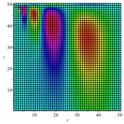 Figure 1
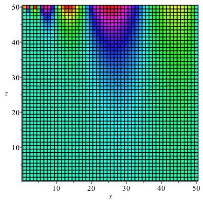 Figure 2
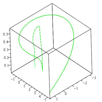 Figure 3
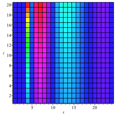 Figure 4
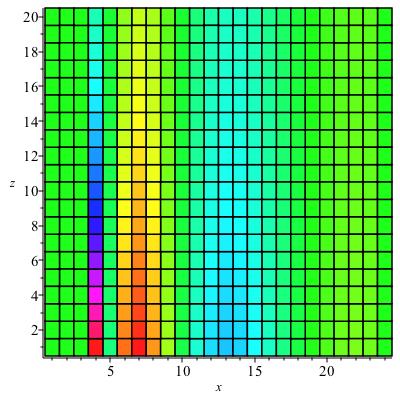 Figure 5
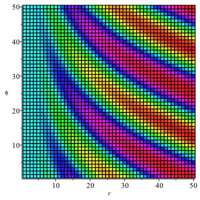 Figure 6
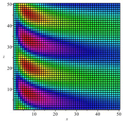 Figure 7
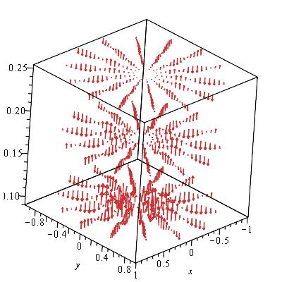 Figure 8
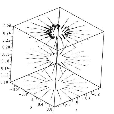 Figure 9
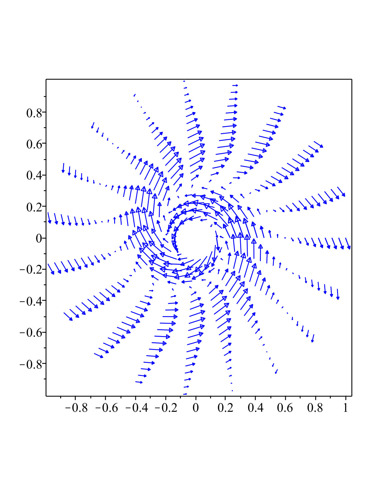 Figure 10
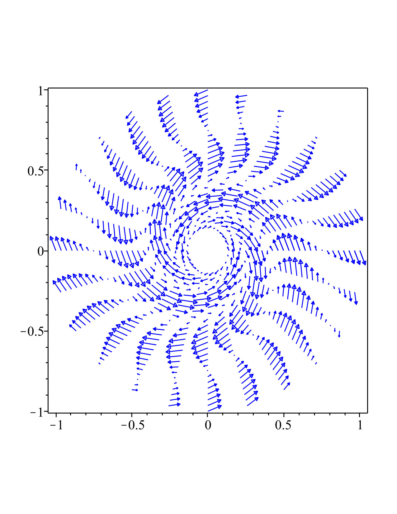 Figure 11
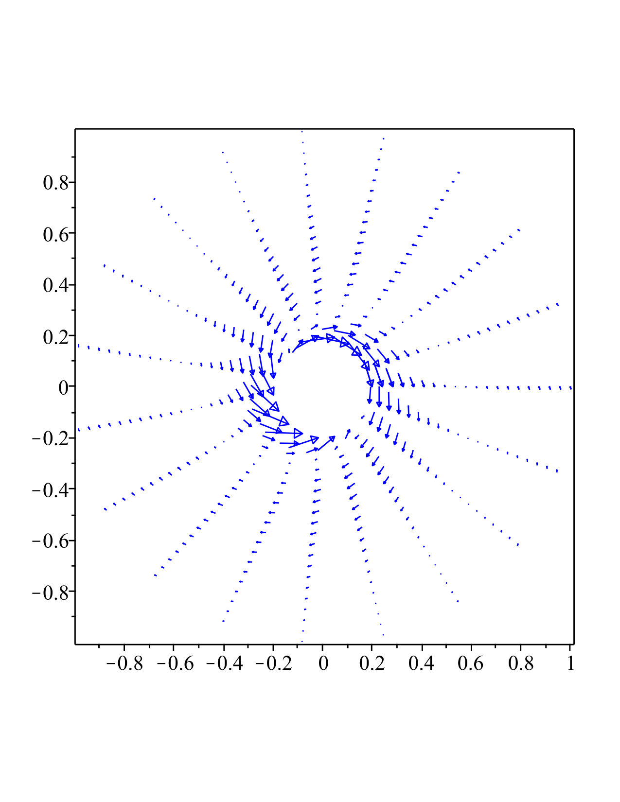 Figure 12
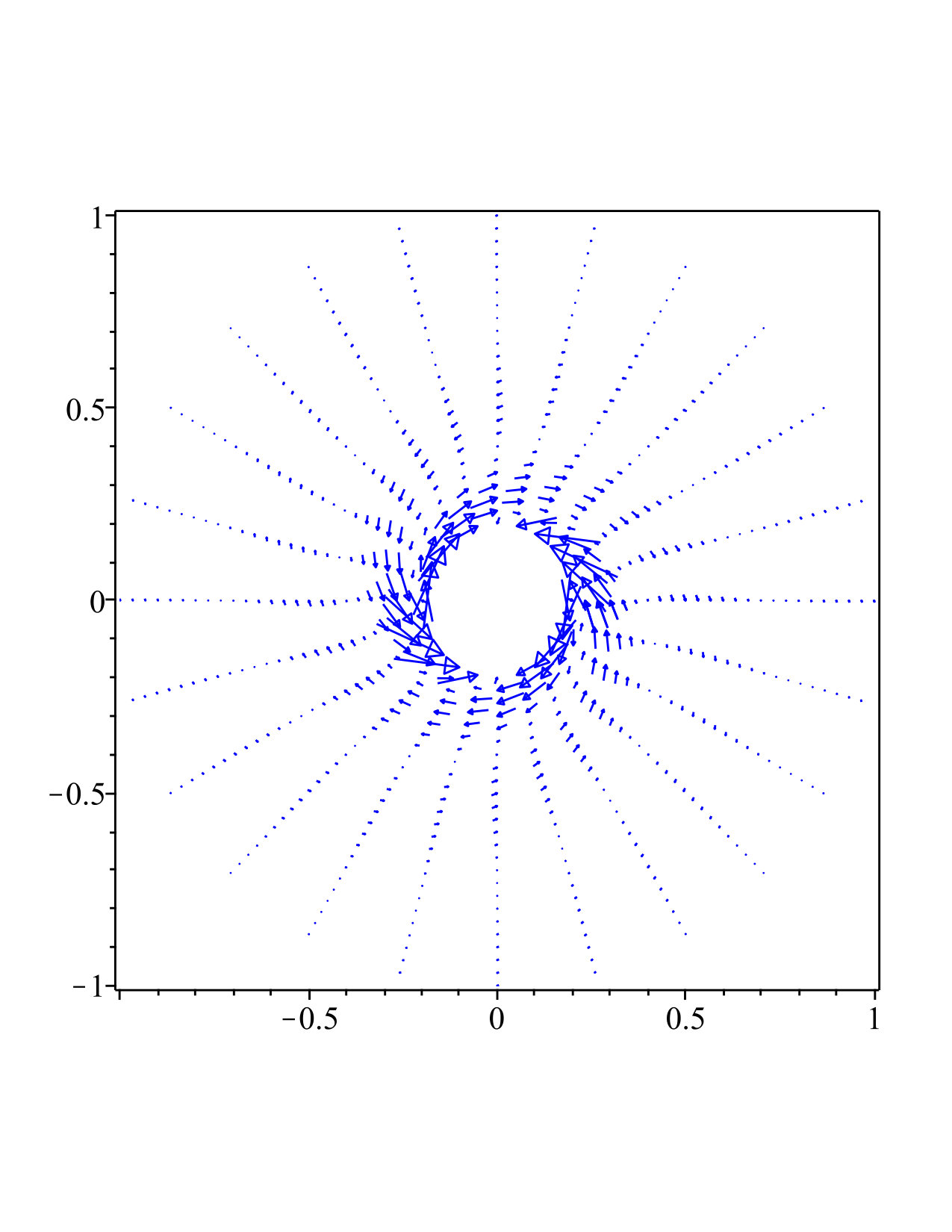 Figure 13
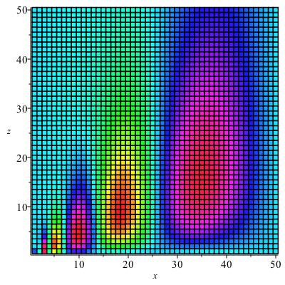 Figure 14
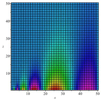 Figure 15
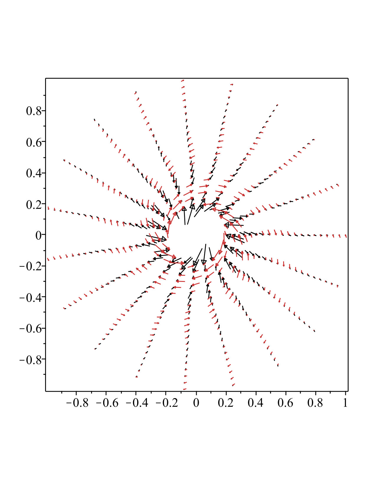 Figure 16
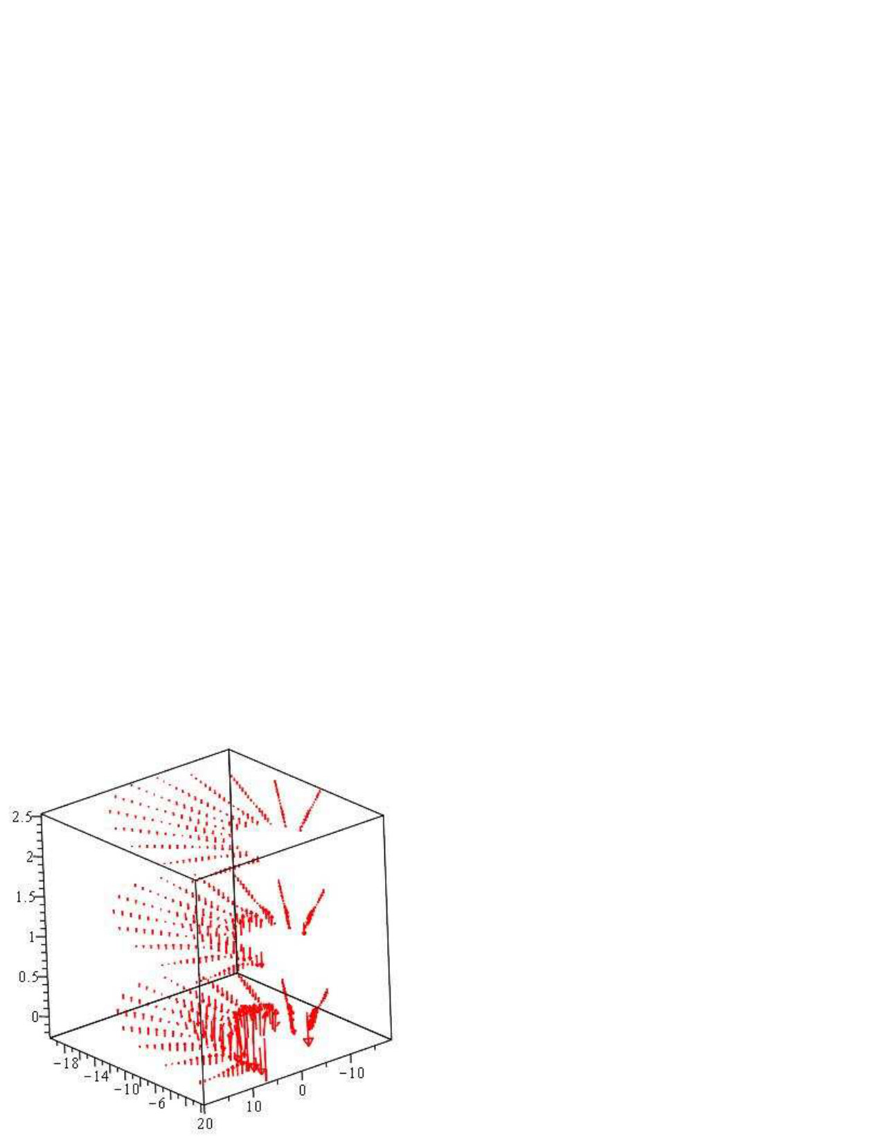 Figure 17
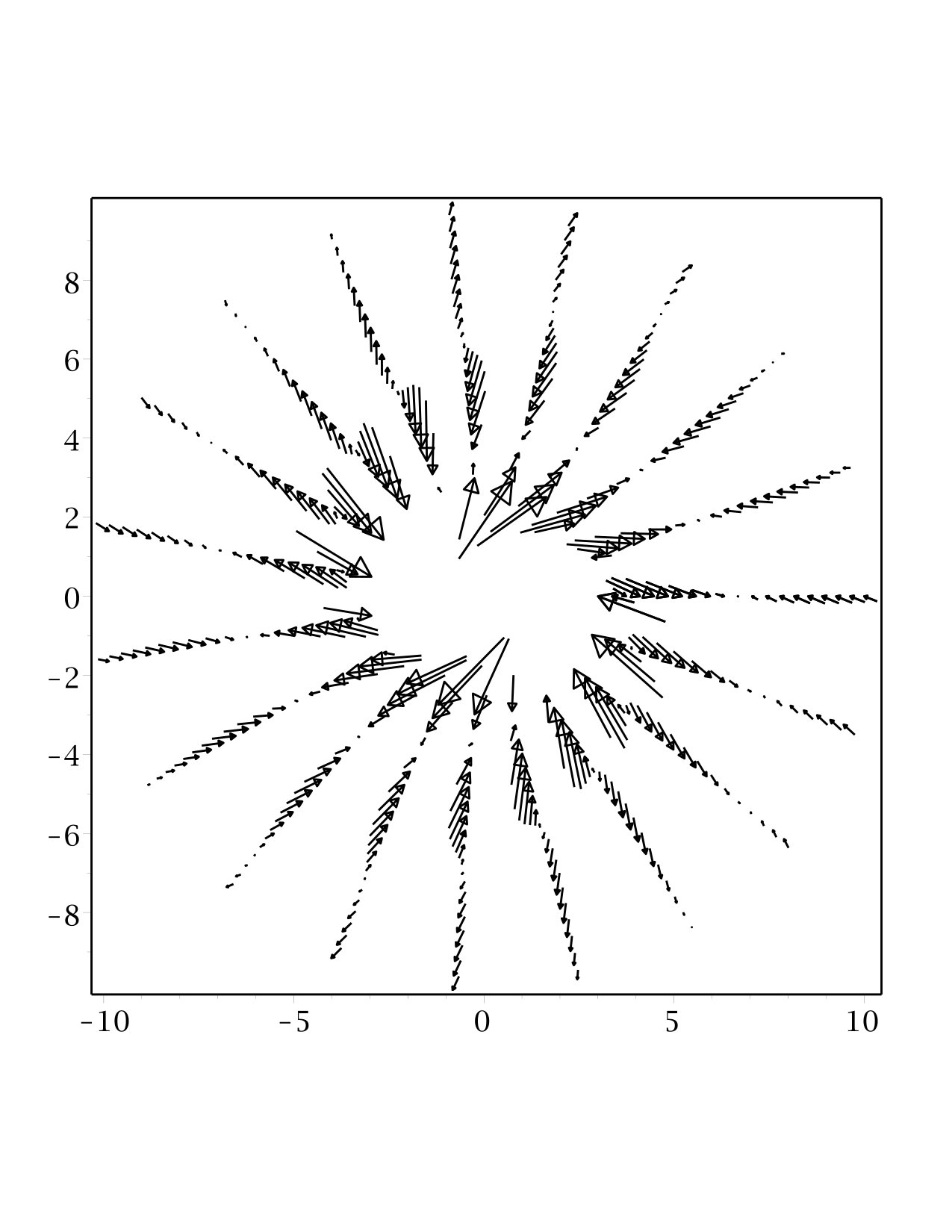 Figure 18
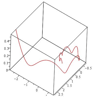 Figure 19
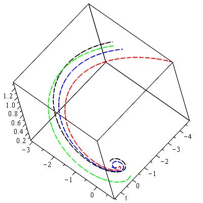 Figure 20
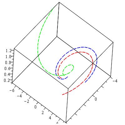 Figure 21
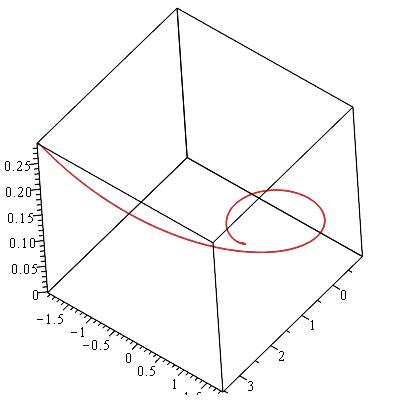 Figure 22
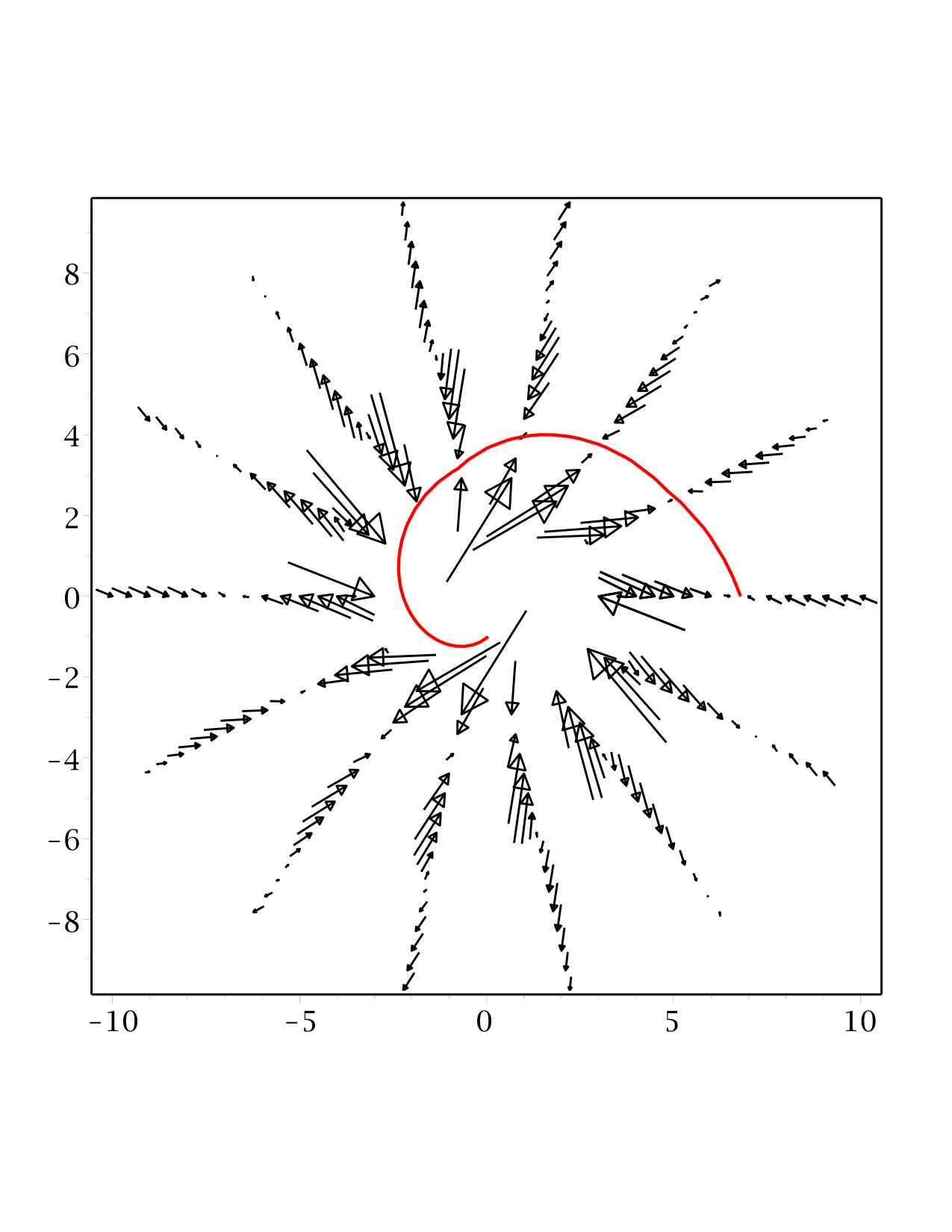 Figure 23
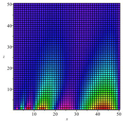 Figure 24
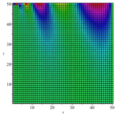 Figure 25
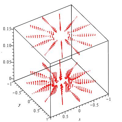 Figure 26
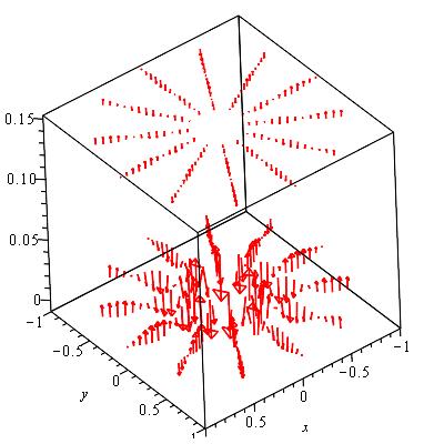 Figure 27
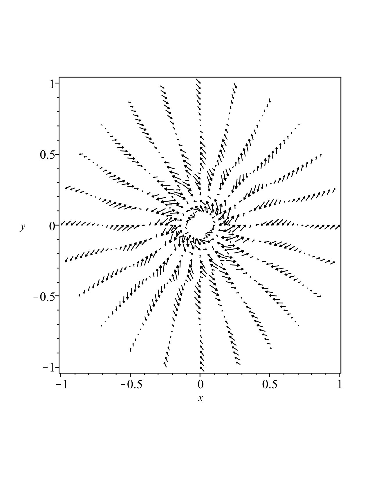 Figure 28
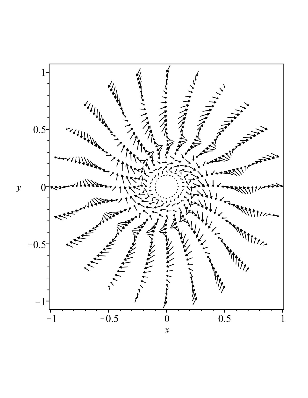 Figure 29
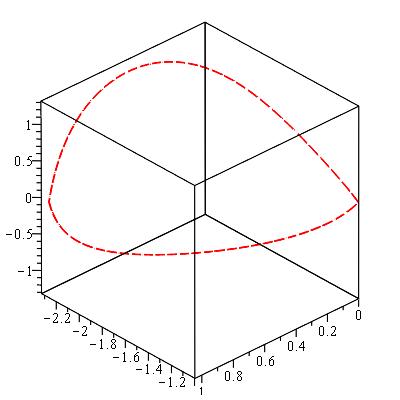 Figure 30
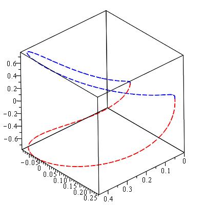 Figure 31
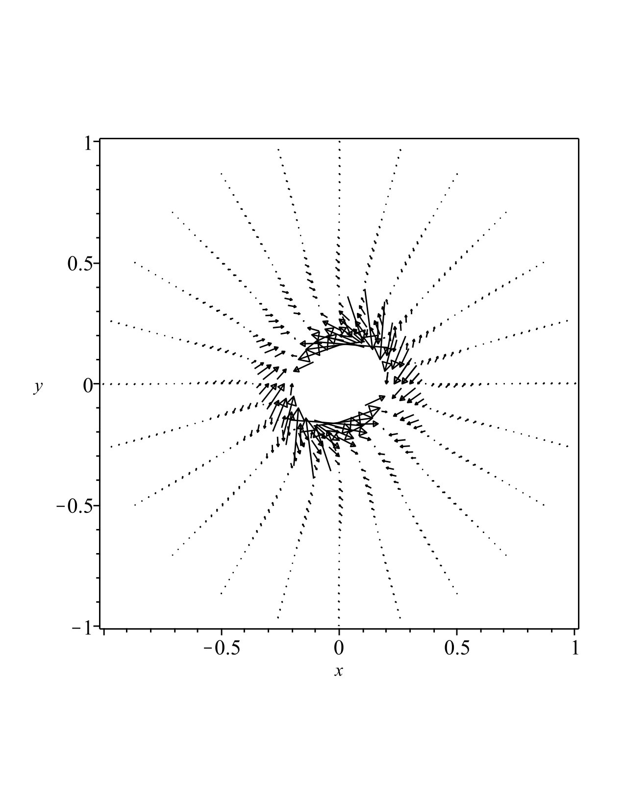 Figure 32
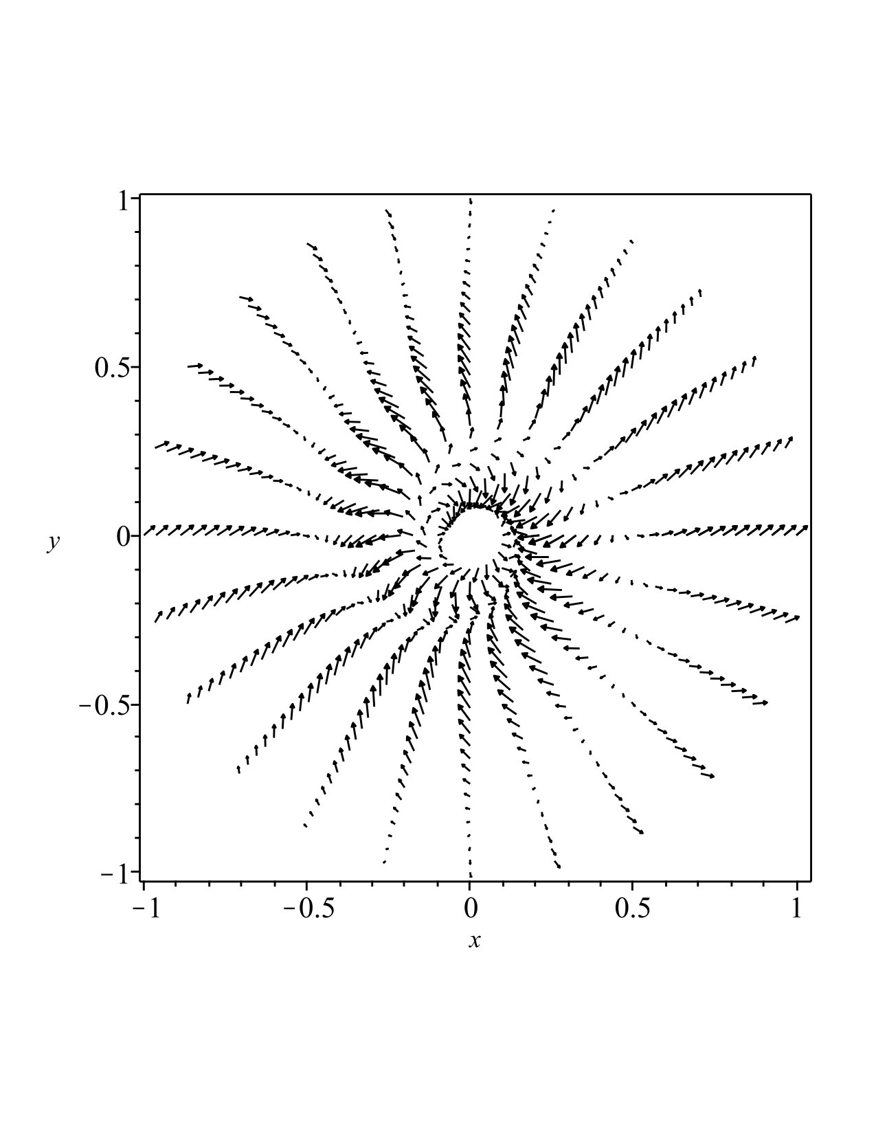 Figure 33
Peer Reviews
No public reviews on file for this paper yet. If you reviewed it on a platform where reviews are public (OpenReview, ICLR, NeurIPS, ICML), you can paste yours below so the community can read it here.
Videos
No videos yet. Explain this paper in a talk, walkthrough, or lecture? Add one.
Magnetic Spiral Arms in Galaxy Halos
R.N. Henriksen1
1Dept. of Physics, Engineering Physics & Astronomy, Queen’s University, Kingston, Ontario, K7L 3N6, Canada [email protected]
(Accepted XXX. Received YYY; in original form ZZZ )
Abstract
We seek the conditions for a steady mean field galactic dynamo. The parameter set is reduced to those appearing in the and dynamo, namely velocity amplitudes, and the ratio of sub-scale helicity to diffusivity. The parameters can be allowed to vary on conical spirals. We analyze the mean field dynamo equations in terms of scale invariant logarithmic spiral modes and special exact solutions. Compatible scale invariant gravitational spiral arms are introduced and illustrated in an appendix, but the detailed dynamical interaction with the magnetic field is left for another work. As a result of planar magnetic spirals ‘lifting’ into the halo, multiple sign changes in average rotation measures forming a regular pattern on each side of the galactic minor axis, are predicted. Such changes have recently been detected in the CHANG-ES survey.
keywords:
galaxies:general, galaxies: magnetic fields, galaxies:kinematics and dynamics
††pubyear: 2016††pagerange: Magnetic Spiral Arms in Galaxy Halos–References
1 Introduction
Magnetohydrodynamic dynamo theory has a long history and a rather rigorous foundation. Reviews of early pioneering fundamental work may be found in (Roberts & Soward, 1992; Kulsrud, 1999) and for astrophysical applications in Ruzmaikin,Shukurov &Sokoloff (1988).
The theory has found perhaps its most testable astrophysical application in the explanation of large scale magnetic fields in spiral galaxies (e.g. Chamandy et al. (2014)). The extended, quasi-transparent nature of these objects allows the components of the galactic dynamo to be observed. This is especially true when a combination of face-on and edge-on spiral galaxies (e.g. Beck (2016) and Krause (2015)) is considered. The systematic study of a sample of edge-on galaxies in the CHANG-ES survey Wiegert et al. (2015) has reinforced the belief in an intimate connection between halo and disc magnetic fields. Such a connection has long been advocated for external galaxies by Krause (e.g.Krause (2015)), and it has been brilliantly demonstrated recently for the Milky Way (Farrar (2015)).
That lagging haloes may be an indication of a magnetic connection to the galactic environment, has recently been argued in Henriksen& Irwin (2016) for a special case ( equal to the Alfvén speed) of the axisymmetric mode. There is in that work a kind of simple ‘dynamo’ acting, which is effected by shearing the magnetic field between the disc and the distant environment. Such lags may also be produced by classical dynamo action. We find here that dynamo action can (but not always) produce magnetic spirals on conical surfaces that extend into the halos of galaxies with decreasing amplitude, just as in Henriksen& Irwin (2016). If the velocity field is simply proportional to the magnetic field, then lags will arise. The dynamo action will also be revealed by oscillations in the sign of rotation measures and/or in the oscillation of polarization intensities, particularly when this occurs in a regular pattern on the same side of the galactic minor axis.
The observations of face-on galaxies imply the existence of magnetic spiral arms (e.g. Krause (1993), Beck & Hoernes (1996) and Beck (2015)). There has been an intensive effort to explain the origin of these arms (e.g. Moss et al. (2013), Chamandy,Shukurov & Subramanian (2015) and references therein) including their location, which is often different from that of the gravitational spiral arms. This effort has been conducted largely numerically, but it has led to a number of innovative physical ideas.
These physical ideas involve among others the variation of vertical outflow and turbulence with respect to the gravitational spiral arms, the notion of a relaxation delay in the ‘alpha’ effect, and the disc/halo interaction. The numerical models have also had to deal with ‘quenching’ of the turbulent alpha effect and dynamical effects due to gravity and magnetohydrodynamical back reaction. Despite these efforts, there does not seem to be a consensus as yet as to the physical origin of the magnetic spiral arms, in part due to the rich collection of parameters.
The present work does not attempt to deal directly with these questions. Rather it provides a simple model for the existing magnetic spiral arms in the hope of minimizing the number of parameters essential to their existence. We assume a steady state and we look for spiral arm solutions by expanding the magnetic field in logarithmic spiral modes. This avoids the ‘quenching’ problem associated with unlimited growth of the field, and by insisting on spiral modes, addresses directly the conditions necessary for their existence. An expansion of these fields into galactic halos is found, although the description is limited to moderate heights above the disc in our general approach. An exact analytic solution extends this behaviour to arbitrary heights.
There are some physical gaps due to our assumptions. Because of the assumed steady state and the modal analysis, there is always an arbitrary constant in our solutions. Hence we can not predict the strength of observed fields, although in principle one can try to fit them globally (or locally in a peculiar region) with that one parameter. We clearly can not discuss growth rates of the magnetic field. Moreover we are forced to discuss the axisymmetric mode (both magnetically and gravitationally) separately, because of the form of the scale invariance assumed. However such behaviour can be added when necessary, and is studied for example in Henriksen& Irwin (2016).
In addition we have to ask in what reference frame is the magnetic spiral steady. We will usually assume that it is steady in a frame rotating rigidly with a pattern angular velocity , which might be that of the gravitational arms should these have a distinct pattern speed. Subsequently, the rotation velocity would be added to the dynamo velocity to yield the observed velocity. In the local inertial or ‘systemic’ frame, the boundary condition on the dynamo velocity is that of the rotating disc at the disc and zero at infinity. In the disc frame the boundary conditions would be rather the reverse, zero at the disc and negative disc velocity at infinity. When the velocity is taken parallel to the magnetic field , we suppose that both quantities are in the pattern frame, which may also be the systemic frame.
Unless the pattern rotation is zero, the magnetohydrodynamics should also be analyzed in the rotating frame. The simplest possibility is to take the peculiar mean velocity in the rotating frame to be Alfvénic and the halo gas to be incompressible Henriksen& Irwin (2016)). A macroscopic equilibrium due to pressure, magnetic, gravitational and inertial forces can then be found straightforwardly. The incompressibility assumption is quite reasonable if the cosmic ray (CR) pressure is dominant in the halo, since the sound speed () implies a wave crossing time that is short on a galactic time scale. This is still true for the hot halo component. However we will not discuss the rotational dynamics in detail in this work. Some discussion of Faraday’s law in a rotating frame is required however, since this is at the origin of the dynamo equation.
Ignoring explicit gas dynamics is a means of surveying rapidly the effects of different flow topologies on dynamos. Although scale invariance is often the asymptotic state of a complex physical system, no rigorous prediction for the velocity field should be expected in this survey. For simplicity we have used a scale invariant class () that corresponds to conservation of specific angular momentum. This implies the somewhat uncomfortable velocity and magnetic field dependence in a pattern frame.It would be more realistic in future work to use the class , which implies a velocity and magnetic field constant in radius in the pattern frame of reference. If however the vertical scale height is much smaller than the radial disc scale, then even for the velocity tends to a constant (e.g. appendix of Henriksen (2017),).
The previous work most similar to our own in spirit is that of Subramanian & Mestel (1993), since they assume a steady state in the pattern reference frame. However it is reassuring that previous numerical work on the time dependent version of our equations has uncovered similar results. These are found for example in Donnor& Brandenburg (1990) and Moss et al. (1993), which are discussed briefly with our conclusions. The steady state and scale invariance together replace many of the parameters adopted in these papers.
In the next section we formulate the equations of the problem under our assumptions. This includes the modal and scale invariant ansätze. In the following section we find the conditions on physical quantities required for an exact scale invariant example. Subsequently we illustrate the steady magnetic dynamo field in and above the galactic disc for several cases depending on the nature of the velocity.
In appendix A we discuss at length the exact scale-invariant equations expressed both in terms of the vector potential and of the magnetic field. These are used to show the transition to the approximate equations that we use for modal analysis in the text.
In Appendix B we introduce the scale invariant Kalnajs (Kalnajs, 1971) model of the gravitational spiral arms, and indicate how these might eventually be coupled to the magnetic spiral arms. Illustrative figures are included in that appendix, as is also a speculation regarding the separation of gravitational and magnetic arms.
2 Kinematic Dynamo Theory
It is worth remembering that the classical isotropic mean-field dynamo theory relies on an inertial electric field that is due to flux-freezing, plus subscale ‘turbulent’ diffusion and generation. This takes the form in Gaussian Units (e.g. Moffat (1978))
[TABLE]
where is proportional to the mean magnetic field and is the mean velocity field. It is convenient to regard the vectors and to be the true mean fields divided by , where is some fiducial gas density. Accordingly, each of these vectors has the Dimension of velocity in electromagnetic Units (emu). We have labelled the subscale alpha and beta effects by and respectively, but subsequently we absorb the beta effect into the subscale diffusion by letting
[TABLE]
Note that there is no electrostatic field included, since that would require charge separation.
In a true steady state in an inertial frame of reference the integral of the electric field around an arbitrary stationary contour is zero by Faraday’s law. Consequently the electric field itself may be taken zero, but for an unlikely electrostatic term. After introducing the vector potential and multiplying equation (1) by , we obtain our working equation in the form
[TABLE]
This is equivalent to the standard form involving the curl of this equation, provided that the electrostatic field is neglected.
One should note that setting equation (1) equal to zero yields the dynamo equations directly in terms of the magnetic field. These equations do not automatically contain the solenoidal constraint unless the substitution in terms of vector potential is made.
The above argument holds strictly only in an inertial frame. In a frame rotating with the pattern speed (primed), Faraday’s law becomes, to first order in ,
[TABLE]
where we have moved to the right hand side of the equation and calculated it explicitly there. Thus, so long as is much larger than a typical scale in the galactic disc and halo, we can neglect the new term on the right compared to the curl of the electric field. The argument above will thus apply approximately to a steady state in a uniformly rotating frame. One assumes that equation (1) and hence equation (3) holds in the rotating frame.
We proceed by seeking a scale invariant solution for the vector potential. Following the procedure advocated in Henriksen (2015). We use the symbols and for reciprocal temporal and spatial scales, each of which may be taken to have Dimension of reciprocal length in a steady state. Then we transform from cylindrical coordinates (referred to the galactic axis) to self-similar or ’Lie invariant’ coordinates according to
[TABLE]
We note that
[TABLE]
so that it is constant on cones whose generators pass through the centre of the galaxy.
The quantity may also be written as
[TABLE]
which shows each constant value of to define a logarithmic spiral having as the tangent of its (negative) pitch angle. If is positive the spirals are trailing relative to the positive sense of . This sense is that of the pattern speed, normally given by the rotation of the galaxy. One can describe trailing spirals with by taking the sense of increasing to be opposite to the sense of galactic rotation.
Strictly speaking our transformed coordinates should be , but the scale invariance reduces them to partial differential equations in and . We give these equations in their exact form in appendix A for possible future use. We also give the equations in terms of the magnetic field in the Appendix, because these allow exact ‘toy’ models to be found.
Our approximate treatment lies in merging the separate and dependence into as in equation (5) and ignoring any other dependence. This is reasonably accurate so long as is small. We have inserted the square root of (i.e. ) in the dependence of the scale invariant quantity , in order that our spiral modes (see subsequently) may have an exponential decline (or increase) with . If is suppressed each node will have a periodic behaviour in and it would require a Fourier sum to obtain a reasonable behaviour in . Although this remains formally a viable option, the exponential decline (and occasionally growth) with distance from the disc for each node at fixed seems more physical and indeed appears naturally in sample analytic solutions. We note that the vertical scale height of the magnetic field is given by the radius at each point.
According to the scale invariant ansätz, we are required to assign a scaling to each physical variable depending on its Dimension. For example, the Dimension co-vector of the vector potential is in the scaling space. This gives its exponential scaling factor as so that (Henriksen, 2015)
[TABLE]
For scale invariance, the dependence on in the scaled vector potential must not appear, since we have chosen it to be along the (Lie) symmetry direction (Henriksen, 2015). Taking into account the various Dimensional co-vectors 111The Dimension of is the same as that of a velocity while that of is the same as that of specific angular momentum and of A and summarizing, our scale invariant ansätz is
[TABLE]
Here we have set the ratio of the arbitrary scales equal to , that is
[TABLE]
which defines the self-similar ‘class’(Carter& Henriksen, 1991; Henriksen, 2015).
We proceed here with spatially isotropic scaling, but different scalings parallel and perpendicular to the disc are possible (e.g. Appendix in Henriksen (2017)). It allows slightly generalized power laws to be the radial power law dependences.
There remains now some tedious algebra in order to transform equation (3) into a useful form using the scale invariant quantities. We give the result for general (after approximation but see appendix A for the complete equations) for reference, but we do not analyze the general case in this work. The equations have only one physical parameter in addition to the similarity class and the velocity components . We take this parameter to be
[TABLE]
which is essentially a Reynolds number ( of the sub-scale turbulence) and is essentially the dynamo number used elsewhere Brandenburg (2014). The velocity components are now in Units of , that is
[TABLE]
Letting a prime denote differentiation with respect to the steady dynamo equations for the vector potential components become at sufficiently small (see Appendix A)
[TABLE]
where
[TABLE]
We proceed by taking the dependence on to be the modal form
[TABLE]
where is a constant vector and . We note that if we wish the magnetic field to decrease with increasing , then and should have the same sign above the plane and opposite signs below the plane. The reverse sign assignment will produce a field increasing into the halo, which we do not exclude ab initio.
In order to reduce the problem to this set of three ordinary equations for the vector potential as a function of , approximation has been necessary. All terms proportional to occurring in the equations (3) if written out in full in terms of the variables and , are neglected (see Appendix A). Moreover a term in has been neglected in the diffusion part of the radial equation (see AppendixA).
One can allow the diffusion coefficient and the Reynolds parameter to depend on , provided the functional dependence is the same for each. That would allow azimuthal anisotropy in the turbulence e.g Subramanian & Mestel (1993). If and have the same dependence on , the equations will not be affected since remains constant. If the velocity terms are present, equation (15) shows that in order for the velocity parameters to be constant (which leaves the equations unchanged), one must have the scaled physical velocity component proportional to . This allows for a velocity that is a power law in radius and varies on cones and logarithmic spirals. It makes physical sense to have all of these functions the same on cones and spirals (near the plane), if all quantities refer to the turbulence generating the dynamo.
In any case we proceed by assuming the parameters to be independent of . Rather than attempt a general solution for , we use the linearity of the equations to make the spiral modal ansätz
[TABLE]
Here is the mode number and the form of is required for azimuthal periodicity.
We will only study the similarity class in this work. This implies a global constant with Dimensions equal to that of specific angular momentum (Henriksen (2015)). Equations (9), (10), (11) and (12) consequently indicate the assumed radial dependences. These are, including the modal ansätz and remembering equations (5) and (7),
[TABLE]
Substituting these dependences into the equations for we obtain the homogeneous modal equations
[TABLE]
which are invariant if and are negative together. The vector constant may be complex at this stage as it contains both phase and amplitude information.
Setting the determinant of the coefficients of these last equations to zero yields the conditions on the parameters for a steady dynamo to exist. An advantage of taking is that only in this case is the divergence of the velocity zero, provided that the set is independent of . This allows the background density to be considered uniform in the steady state if the velocity is non-zero. However we do not solve the dynamical problem in this paper.
We will proceed with the approximate modal analysis of the steady dynamo in the section below. In appendix A we show the exact equations and the nature of our approximation. In Appendix B we introduce the spiral modal analysis of gravitational arms. This analysis is well known (Binney& Tremaine, 2008), but not as a scale-invariant class.
3 Steady Dynamo Examples
An Exact Analytic Example
We find an exact analytic solution of the scale invariant magnetic field equations given in Appendix A. The solution is solenoidal and is easily stated implicitly in its complex form, but the real parts are complicated so that we omit these explicit expressions for brevity . Our main concern is to show that this exact solution contains similar behaviour to that which we find below in our approximate treatment with more general parameters.
The solution is found with and the scaled radial velocity . Moreover we anticipate our approximate results by setting . This gives radial infall in a pattern frame according to . We remove the dependence from equations (A68), (A69) and (A70) by setting . Then these equations yield:
[TABLE]
These equations are linear and are readily solved for the complex forms. Here we consider only the azimuthal equation, for which the exact solution is
[TABLE]
where is a complex constant. If we treat as small, expand this result, and restore the dependence we obtain
[TABLE]
Thus on taking the real part, the exact solution reduces in this limit to modes that are either exponentially damped or growing (depending on whether is positive or negative) with . Moreover these oscillate in and , which suggests twisted loops near the plane. This is form that we find also in our approximate procedure, which procedure allows a more general choice of parameters.
The general Approximate Case
We have to solve the homogeneous equations (26). (27) and (28) for the amplitudes of the dynamo vector potential. In fact we can only find two ratios, which leaves us with the expected arbitrary constant. This is only possible if the determinant of the coefficients of these equations is zero, which gives us the restriction on our parameters for a steady state to exist. The determinant condition takes the form of a cubic for with complex coefficients depending on the velocity components, namely
[TABLE]
We recall that and may be the same arbitrary function of , given this dispersion relation. From equations (10) and (15) we see that the physical velocity may also be the same function of multiplied by , provided that the scaled velocity components are constant.
The general case is found by setting the real and imaginary parts of equation (34) equal to zero and requiring a real solution. These conditions become
[TABLE]
Combining these two equations yields finally another equation for in the form
[TABLE]
which must hold in order that the from first of equations (35) be a root of the second of these equations. It is not necessarily a root of the equation (36) however. For that to be true there is a restriction on the velocities found by inserting the value of from equation (35) into equation (36), which takes the form
[TABLE]
This consistency condition must be checked in each special case below. One has also to insist on an integer mode number.
We note that the combination is proportional to the velocity parallel to the magnetic spiral arm in the plane ( is proportional to the velocity perpendicular to the magnetic arm). Both signs of the square root are possible. Rather than pursue the solution for the coefficients in the general case, we look at some simpler limits in this work. One should recall at this point that the velocities are in a pattern frame of the magnetic structure. Only if we place ourselves in the systemic frame will the azimuthal velocity correspond to the galactic rotation velocity.
All velocities are zero or parallel: Case A.
Here either is zero in the pattern frame or . Equation (36) gives immediately that (as in our sample analytic solution), but the first of equation (35) shows that we must extract the positive root here so that
[TABLE]
Hence a steady, stationary (zero velocity in the pattern frame), dynamo requires the turbulent (helical) Reynolds number to be equal to plus or minus the mode order. This corresponds to magnetic field that is either decreasing or increasing with respectively. A mode determination would thus give directly the value of this quantity, which can be expected to be of order unity.
The helicity will change sign across the disc with the mode number , if a direction is assigned to this quantity by (say) a right-hand rule relative to the positive direction of . A change in sign then yields the same handedness relative to the rising direction on crossing the galactic plane. We assume a positive diffusion coefficient.
Only an azimuthal velocity is present: Case B
This case allows for an dynamo in the pattern frame of reference. Formally equations (35) and (36) give
[TABLE]
However reconciling the two values of is found to require ()
[TABLE]
which is not possible for real ,,. We conclude that there is no steady pure dynamo (identifying with the background disc velocity in the pattern frame), unless
[TABLE]
The helicity will again change sign across the plane with the change in .
Only a vertical velocity is present: Case C
This case has some considerable interest since a vertical velocity is often required to quench the evolution of a turbulent dynamo.
Conditions (35) and (36) become
[TABLE]
Eliminating between these two expressions gives ()
[TABLE]
so that the ratio of alpha velocity to diffusion velocity is again
[TABLE]
One can change from infall to outflow by taking above the galactic plane. However then we find the strength of the magnetic field increasing with positive . This is effected below the plane by taking . Antisymmetry for the tangential magnetic fields applies to both infall and outflow (see below) on crossing the plane. The vertical velocity is scaled by the diffusion velocity , which has a certain arbitrariness due to the choice of turbulent scale .
Only a radial velocity is present: Case D
In this case we have from equations (35) and (37) that ()
[TABLE]
Therefore we have only a very restricted steady dynamo wherein and the radial velocity is slower when directed radially outward. The excluded case satisfies all of the requirements with . It corresponds to our exact example.
We turn in the next section to the form of the magnetic field in terms of the complex coefficients . In this section we have found general conditions on the parameter and the scaled velocities under which a steady dynamo (‘kinematic’, because the velocities are used as parameters) can exist.
4 Magnetic Field Structure
We calculate the magnetic field from equation (22) and . We take the real part. We usually take the arbitrary constant to be real and equal to . In that case we find the field (divided by for arbitrary density ) in the form
[TABLE]
The real and imaginary parts of the coefficients are indicated explicitly. It is readily shown numerically that this magnetic field is divergence free to one part in for any particular set of parameters and any particular location in space. The behaviour crossing the galactic disc depends on the behaviour of the coefficients at this transition. In many cases however we find that the tangential magnetic field changes sign with and changing together, while the vertical field remains continuous. This changes the handedness of the magnetic field across the plane.
4.1 Zero Velocity Steady Dynamo Field Structure: Case A
This is the pure dynamo with diffusion. It stands in contrast to the dynamo with diffusion that arises with non-zero .
In the general modal analysis, the exponential decline (or growth) from is only one way in which the disc is present. There is also the question of boundary conditions. Two possibilities arise. In one case all components of the magnetic field are considered to be continuous. The magnetic field at is then identical to that at . This is the symmetric boundary condition. We do not find this possibility in this pure example.
In the second case the vertical field is continuous but the tangential magnetic field is anti-symmetric across the disc such that at . In order to arrange this with spiral modes we find that one must hold the switch constant at while changing the sign of and (hence also ). This is because the determinant that yields the coefficients and when (or zero) is invariant when crossing the plane under this condition. The vertical component of the field is properly continuous, but its derivative changes sign according as the plane is approached from ‘above’ or ‘below’ the plane. In an average sense , which one expects with this boundary condition on averaging the continuity equation.
A closed magnetic field loop can be constructed for the anti-symmetric boundary condition by calculating the arc above the plane from a first crossing of the galactic plane to a second crossing. Then one changes the symmetry of the field (which reverses the direction of increasing arc length) and computes the arc below the plane that returns to the first crossing of the plane. We illustrate this in the figures.
Having confirmed that the determinant of the coefficients is zero, equations (26), (27) and (28) are readily solved for and as
[TABLE]
By taking the real and imaginary parts of these expressions, we determine from equations (46), (47) and (48) the magnetic field at any point to within an arbitrary multiplicative quantity . We recall that is an amplitude of the azimuthal vector potential and has the Dimensions of this potential. Figure (1) shows some aspects of the magnetic field structure in the galactic disc at .
In figure (1) we show vectors near but above the plane, for on the left and on the right. In each case . We see that the fields vary rapidly in , radius and azimuth. The variations in radius and azimuth are correlated with the location of the arms, as may be seen by examining the arms in figure (2). There is a suggestion that the field must connect in loops over the arms, but the tangential field is concealed in the figure by the stronger vertical component. Nevertheless, a careful inspection of the figure does show rapid variation in the sign of the field vector associated with loops near the plane. We illustrate these loops in figure (2).
We observe that the field strength falls off faster in at smaller as expected from the scale height in the self-similar form. The mode falls off generally more quickly in than does the mode. The extent to which spiral structure is ‘lifted’ into the halo is important for the rotation (and polarization) measures of edge-on galaxies. Normally the complete field will include an axially symmetric () component, which has been treated in a companion paper.
The bottom left image in this figure shows a two-armed spiral with positive helicity () at . This produces magnetic ‘polarization arms’ wherein the magnetic vector is at a considerable angle to the spiral arm axis. The figure at bottom right differs from bottom left only in having a negative mode number. The arms are still mainly polarization arms at large radius.
At upper left in figure (2) we show a cut through the magnetic halo at , as produced by the dynamo. The pitch angle is . At upper right the image shows the same cut for , , and the same pitch angle. This illustrates a case where the magnetic field is increasing with increasing , most rapidly at small .
In all cases the strongest magnetic structures are not magnetic arms in the sense that the magnetic field lies along the arm. They are rather ‘polarization’ arms where the linear polarization (for a face-on galactic view) would be strong in a spiral pattern. Since some of the vectors must lie on loops above the plane, we can also expect variations in Rotation Measure (RM) over the plane. The loops calculated in the lower part of the figure extend over large regions of the plane and over the arms. Such loops manifest zero divergence. There should be RM variations on the same scale.
The field line loops shown in the lower part of figure (2) are calculated according to
[TABLE]
where is along the field line. The sense of increasing arc length () will coincide with the increasing direction of the tangential coordinates, when the tangential field components are positive. These loops must be regarded only as illustrative since the full magnetic field comprises an infinity of such loops. Their existence seems certain, but because of our approximation we can not really follow them to heights greater than a kiloparsec or so above the plane. The loops shown in the figure are pushing the approximation. Nevertheless this structure seems to be characteristic of a pure ‘alpha squared’ turbulent dynamo as discussed in this section. The topology has observational consequences.
Additional observational consequences follow especially for edge-on galaxies (e.g. Mora Partiarroyo (2016); Schmidt, Partiarroyo & Krause (2016)). We take a simple model of a cylindrical halo that has the same radius as the galactic disc. We assume the inclination of the galaxy to be and calculate (using the dynamo magnetic field)
[TABLE]
along the line of sight, distributed over the halo. In order to isolate the effect of the dynamo magnetic field, we take the electron density to be constant. This is easily changed in order to deal with observed cases. The radial variation of the electron density is probably the most important additional parameter, because we are constrained to be near to the plane. We show the first and second quadrants (the galactic minor axis is the ordinate) in figure (3) for the mode with the pitch angle of .
This quantity that we call rotation measure (RM) is only truly relevant to a Faraday screen with no internal sources. This is not the quantity that is found by the application of rotation measure synthesis. One should ultimately integrate the equation of radiative transfer through the halo and calculate (, are the Stokes parameters) for the exiting radiation. For an optically thin halo this is quite feasible, but we must leave it to a more observationally oriented work. Small pitch angles approach axial symmetry, and in that case the RM may be considered as that produced on emission at the tangent point to a true magnetic spiral arm.
We see the anti-symmetry across the disc in figure (3) that is characteristic of these ‘zero velocity’ modes. The mode has fewer reversals, but these extend to larger so we have not shown them here in view of our approximation.
The second and third quadrants are readily generated by rotation about the galactic axis (on the left edge and upward) using the left-hand rule. Subsequently the colours must be interchanged. This produces diagonal symmetry over the whole halo. The positive or negative sense of the colours can also be interchanged by changing the sign of the amplitude constant .
In figure (3) the abscissa gives , so that one Unit radius is the radial extent of the disc. The ordinate shows , so that the halo extends to only half the disc radius and the structure lies within our approximate region. The absolute magnitude of this Faraday screen RM requires fitting a multiplicative constant to the data. However the contrast in amplitude of peaks of different signs varies along the disc in the range from to . Corresponding variations in the polarized intensity in the halo should also occur, with peaks anti correlated with theRM peaks. Observing such variations can vastly improve our knowledge of galactic halo magnetic fields.
In cases where at positive , the contrast in RM between the arms can be very great, as seen at upper right in figure (2). Detectable RM oscillations may only be visible at large radius.
4.2 Dynamo with Azimuthal Velocity only: Case B
This case comprises a simple mean field dynamo. It is particularly simple to find the complex coefficients that determine the mean magnetic field. These are
[TABLE]
The calculations reveal that it is with and that true magnetic arms are produced. The positive mode number and positive give only polarization arms. There is a case with the magnetic field increasing with wherein and . Should one obtains very strong true magnetic arms only at small radius. The contrast in the RM oscillation amplitude that results is very large, so that one sign is likely to be undetectable. The , case gives only strong polarization arms.
The RM produced by the mean field when and is rather similar to forms found below in case C. In particular the , mode RM is almost identical to that of figure (9) regarding oscillation on the same side of the galactic minor axis, so that we do not repeat it here.
Moreover the magnetic field above the disc forms high loops in our calculations. Figure (4) shows a loop extending to large radius (solid line) for the , mode, plus a smaller loop (dashed line) present in the , mode. The latter field increases with increasing . Both field lines start at the disc at the same azimuth and radius, but the dashed loop rather quickly moves to the centre of the galaxy, where it crosses the plane. We do not pursue this case further here, but when fitting data it should be combined with case C as studied below.
As a corollary to this section, the assignment also allows a dynamo that includes vertical outflow. The parameters are :
[TABLE]
The coefficients required in order to calculate the magnetic field are
[TABLE]
This case is likely to be prominent when fitting observed data, but in the interests of brevity we do not study it in this introductory paper.
4.3 Dynamo with Velocity Perpendicular to the Galactic Plane: Case C
This case includes the effect of gas either falling onto or ejected from the galactic plane (above or below the plane), according to and . That is, taking , and allows gas to be flowing out of the plane, while describes accretion onto the plane with. Below the plane we must have for outflow and the reverse for inflow.
Once again, having first set the determinant of the coefficients equal to zero, equations (26), (27) and (28) are readily solved for and in the form
[TABLE]
We are now able to find the magnetic field by taking the real and imaginary parts of these quantities and substituting these into equations (46), (47) and (48).
Figure (5) illustrates the behaviour of the magnetic field when only a vertical velocity field is present (recall that it falls off as ). The magnetic spiral, resulting from a cut through the halo magnetic field at , shown at upper left is strikingly well defined as a ‘magnetic arm’ . The mode is and . so that and hence the helicity is also negative. The gas is flowing into the galactic plane in this example. The contrast with the polarization arm from the same cut seen at upper left in figure (2) is marked. True magnetic arms are never globally produced in the zero velocity case, whatever the sign of the helicity. This appears to be an important physical distinction favouring an dynamo.
On the right of the figure we show the two-armed spiral (, ) resulting from the same cut and having the same parameters. The accretion and the negative helicity ( ) has produced again very well defined magnetic arms . The cut is at , where is the disc radius. In the two bottom figures of figure (5) we find one and two-armed spiral cuts with outflow ( but for ). In these cases the magnetic field is increasing with increasing , perhaps being carried up by the outflowing wind. The helicity is positive. They are true magnetic spiral arms. The major difference from accretion fuelled arms, is that these arms vary extremely rapidly in strength with radius. Rotation measure variations would then be very difficult to detect as we illustrate ultimately in figure (10) for the edge-on outflow.
The difference between two-armed halo magnetic fields with inflow or outflow is explored in three dimensions in figure (6). On the left we have the field vectors for the mode at to . The pitch angle is as usual and there is accretion with negative helicity. The field is complicated in the extreme, with what appear to be looping field lines over the arms seen in the cut shown at upper right in figure (5). We show this complicated behaviour for one line in figure (7) near the disc.
The contrast with the outflow (and positive helicity) case on the right of figure (6) is of considerable interest. The outflow field is simpler but grows rapidly with height at small radius. This is the source of excessive contrast in the rotation measure. This is in general agreement with the idea that the outflow removes magnetic flux from the galactic disc. Although it may not be evident at this angle in the figure, there is an ‘X type’ projected magnetic field in this image. It is likely to be the field that dominates ‘X type’ behaviour however.
Figure (7) integrates some magnetic field lines using the same field line equations as in the zero velocity example, but with the magnetic fields adapted to this case. At upper left we show a cluster of field lines for the mode , inflow. All of the lines begin at a height of (in Units of the disc radius) . Three of the lines begin at at angles [math], and . The fourth line begins at and . Even though the full height reached by the lines exceeds our approximation limit, the indication is of a smooth spiralling magnetic field rising from the disc and wrapped on cones.
At upper right the cluster of field lines is for the two-armed accretion and . They are identified passing through the height . Two begin at radii at angles [math] and , and the third begins at at zero angle. Once again the indication is of a magnetic field rising smoothly on conical helices. This holds even if one begins the field line very close to the disc, as is demonstrated for this mode at lower right. This is in remarkable contrast to the field line at lower left, which is found in the , ( ) inflow mode. The line begins at , and , the same height as for the image at lower right. Here the change in mode sign has produced a magnetic field close to the disc that loops over the disc extensively, before moving off to greater heights. The loops are sufficiently near to the disc that our approximation should hold. Thus loops of this type would give small scale oscillating rotation measures, which can imitate Parker instability. It may actually physically imitate the Parker instability because we do not detect this behaviour without inflow.
The field lines for the outflow modes are rather complicated and need an expanded study to do them justice. Low loops starting near the galactic plane seem common, however.
We look once again at the ‘rotation measure’ (RM) produced in the halo by this dynamo magnetic field. As in case A we really calculate the isolated effect of the dynamo magnetic field in a Faraday screen with constant electron density. Figure (8) shows the two-armed halo with , infall. As before the halo is cylindrical with the disc radius, and the inclination of the galaxy is . The second and third quadrants maybe found by rotating about the left edge of the figure according to the left-hand rule. Subsequently the colours are interchanged. The electron density is constant, but it should be used to cut off the behaviour in , which rises to the limits of our approximation. The horizontal axis runs from to as before, while the vertical axis runs from to . The antisymmetry is evident on crossing the plane.The Unit is one disc radius.
In figure (9) we show the rotation measure for the two-armed inflow mode , . The peak RM is much closer to the plane compared to the positive mode in figure (8). The same interchange symmetry and rotation allows the construction of the second and third quadrants as previously.
Compared to the mode , mode found in case A, figure (8) shows smaller azimuthal magnetic field near the disc. This is consistent with the low altitude looping field seen in figure (2) and with the smooth, slowly spiralling field lines seen in figure (7).
Finally having the halo magnetic fields consistent with a steady dynamo with outflow allows us to consider the ‘rotation measure’ (i.e. Faraday screen) as seen for a face-on galaxy. We assume it to be perfectly face-on and integrate over from to , taking into account the symmetry of the vertical field above and below the plane. The calculation essentially sees a halo Faraday screen produced by the halo in front of the disc emission. We show a preliminary plot in figure (10) of the inflow mode , . The abscissa is again the radius running from to . The vertical axis however is the azimuthal angle running from radians to radians. The image is then approximately topologically periodic with top edge to be joined to the bottom edge. This can be done by rolling the figure about the horizontal mid-line. Each half of the figure in the vertical sense corresponds to half the galaxy on the sky.
The spiral magnetic structures of alternating sign run from large azimuth at small radius to large radius and smaller azimuth. However the location of the zero azimuth on the galaxy is an arbitrary choice. The cause must be attributed to the looping magnetic field associated with the spiral arms. One expects then an anti correlation with the polarized intensity, and indeed with the location of the magnetic arms as seen in face-on galaxies. Distinct rotation measure patterns such as these are likely to be confused by local stellar sources of magnetic field and /or electron density. We can hope that global averages may be less sensitive to such perturbations. The mode , is similar but has only one rotation measure arm (of opposite sign) on each side of the minor galactic axis. This behaviour is in addition to the small scale RM oscillations to be expected for infall modes.
Remarkably such behaviour may have already been observed in IC342 Beck (2015). On the left of figure of that paper we find the RM plotted over one half of the face-on galaxy. The observed oscillation is much as we expect qualitatively from the left images in our figure (10) . The observation will have to be fit quantitatively, but the fact that the positive and negative amplitudes are observed to be similar is typical of the model result. Moreover on the right of figure we find the polarized intensity (PI) plotted over the same sector. At least where the RM is largest, we see the expected anti correlation with the PI. This must be regarded as encouraging. Figure of that paper shows a striking global magnetic spiral much as we find in our outflow/inflow model.
The right-hand side of figure (10) shows the outflow mode and (depending on whether ) from an edge-on galaxy. The contrast with the previous inflow modes is marked. The radius (abscissa) runs over where the disc radius is Units. We have taken the upper limit in to be , which is also the maximum in . The second and third quadrants can be found by rotation about the left edge of the figure according to the left-hand rule and subsequently interchanging the colours. The grid is only in this image because the first four units on the abscissa should be blanked.
The important difference from the accretion modes shown earlier is the strong increase of magnetic field with height associated with the outflow. The figure should be compared to the inflow RM found in figure (9). Had we continued this figure to a tenth of the galactic radius rather than one sixth as in the figure, one would find very strong RM at large . This would render the rest of the oscillations difficult to detect. Hence we must look for the behaviour shown in the figure at large radius so that is small. The current contrast is already seen to be large between the upper left and lower right of the figure for positive .
5 Discussion and Conclusions
Using scale invariance symmetry we have expanded steady mean field dynamo solutions in logarithmic spiral modes. The results may be considered to hold either in an inertial frame, or in a locally rotating ‘pattern’ frame. The application of these solutions above the galactic disc is restricted to regions where the tangent of the (complementary) conical angle is small, but an exact solution agrees in the over lap region.
The scale invariance also substitutes for the dynamics in this model. However one should recall that systems far away from initial conditions and spatial boundaries are often in a scale free form. Thus, although the dynamo fields are kinematic, the power law velocities may not be so unrealistic. Moreover the helicity and diffusivity spatial dependence is also dictated by the scale invariance. Our results are independent of arbitrary dependences on of the helicity and and diffusivity, provided these are the same. This dependence is also communicated to the physical velocity through the diffusivity. It is not unreasonable that these dependences should be the same if they are due to sub-scale turbulence.
The gravitational field is an essential part of the ultimate dynamics and in Appendix B we have given the exact gravitational field of a logarithmic spiral in a uniformly rotating pattern reference frame following Kalnajs (1971). To these spiral perturbations one must ultimately add an axisymmetric gravitational mode, perhaps approximated by an isothermal dark halo and a Mestel disc as in Henriksen& Irwin (2016). The addition of magnetic, inertial and pressure gradient forces will complicate the dynamical problem. It seems that this system has not yet been simulated elsewhere.
One should note that the new perspective presented in this Appendix is that this gravitational spiral is also scale free (cf Binney& Tremaine (2008)). This perspective allows some speculation regarding the relative evolution of the gravitational and magnetic spiral arms. In particular there is a prediction that the magnetic and gravitational arms may cross in some cases.
Our approximate formulation for the scale invariant magnetic dynamo is summarized in equations (16), (17) and (18). These require to be for validity, as is shown in Appendix A, but they allow general parameters. They are a function of the single variable (5). A more general scale invariant form requires and to be independent variables and leads to the partial differential equations given in appendix A.
For a particular choice of radial velocity and ‘dynamo’ number, an exact solution was found. This solution justifies our approximate solution in the over lap region and extends the spiral magnetic fields well into the halo. In general this can not be done.
Under the approximation the modal and scale invariant ansätze lead directly to the homogeneous modal equations. The vanishing determinant of these equations yields our major constraint on a steady mean field dynamo in equation (34). This gives the Reynolds number of the sub-scale turbulence (i.e. the dynamo number) that is required for the existence of a steady dynamo as a function of the scaled velocities (also parameters), the magnetic spiral pitch angle, and the mode number. Subsequently we studied three particularly simple special cases for their observational consequences.
The steady dynamo with zero velocity in the pattern frame or with velocity parallel to the magnetic field was our first example.
The Reynolds (dynamo) number is equal to the mode number multiplied by . A negative value implies that the sub-scale helicity is negative. We have looked at cases with both positive and negative helicity. In neither case are true global magnetic spiral arms produced, rather they are polarization arms. This is illustrated in figures (2) and (1).
Figure (1) also shows the magnetic vectors near the plane ( small) in three dimensions. There is a strong indication of magnetic loops associated with the magnetic spiral arms for the mode. Two such loops are illustrated in figure (2). These are characteristic of the steady alpha-squared turbulent dynamo. These loops are seen at small radius to close near the plane. Nevertheless they extend over large regions as a mean field, and they might be detected with suitable data smoothing at larger radii.
The bottom images in figure (1) are of a , accretion mode on the left and , accretion on the right. We see mainly global polarization arms in each case.
Each spiral mode must ultimately be combined with a related axially symmetric () solution. In the combination we expect both the ‘X-type’ fields seen in polarization, plus oscillations in rotation measure (RM) and polarization intensity, to be produced. Halo lag as in (Henriksen& Irwin (2016)) may also be produced in this combined field, on using the appropriate boundary conditions at the disc and at infinity.
It is characteristic of the magnetic fields produced by the steady mean field dynamo of this paper, that the tangential fields change sign on crossing the plane (3), (9). This allows the perpendicular field to be continuous there. In the axially symmetric field, it is possible to have a kind of ‘quadrupole symmetry’ wherein . This is not possible for these non-axially-symmetric modes.
In order to illustrate what might be possible observationally, we have calculated in figure (3) the ‘rotation measure’ (Faraday screen) given by our halo magnetic fields when integrated along the line of sight. The electron density is held constant in order to isolate the mean field magnetic effect. Nevertheless the figure illustrates a new observational possibility, that of oscillating RM sign on the same side of the galactic minor axis. Only the contrast in amplitude between the positive and negative RM peaks is fixed by our calculation, because there is an arbitrary multiplicative constant in the magnetic field. The angle by which the RM peaks emerge from the plane indicates substantial azimuthal field at the disc, originating in the closed loops of figure (2).
We note that this lifting of spiral arms into the halo of the galaxy has also been found in earlier work Moss et al. (1993), although the observational consequences were not greatly elaborated. Figures , , and of that paper are relevant to the present work. We note that they used the same classical dynamo theory as do we, except that they follow its temporal evolution, beginning from some arbitrary ‘seed’ magnetic field. There are certainly times where the magnetic field resembles that found in our steady state approach. Figure indicated that field anti-symmetry across the equator that we also find. Figures and illustrate the transitory lifting spirals. Figure illustrates the sign changing RM in the equatorial plane. The axially symmetric field seems to dominate asymptotically, which is the subject of our companion paperHenriksen (2017). These authors obtain only a qualitative fit to the magnetic field of M81, as is our current objective.
Very similar results are found in the paper Donnor& Brandenburg (1990). Once again rather particular assumptions are made about helicity and diffusivity and angular velocity. The field behaviour (particularly the field lines) is very similar to what we find here. These authors have in addition calculated the RM ,much as we have done, but lying along the galactic plane. The behaviour predicted is compatible with our own predictions, which in our case extend above the plane.
All these authors have used, physically motivated but arbitrary, forms of the variation in diffusivity, helicity and halo velocity. These quantities, coupled with the uncertain seed field, suggest that asymptotically these parameters are not so important. We have avoided many of them be assuming a steady state and scale invariance as the asymptotic state.
Our conclusions based on this example are:
Magnetic Spiral Arms produced by the pure alpha-squared dynamo are mainly polarization arms.
The magnetic field structure associated with the galactic plane continues into the halo. Disc spiral structure is ‘lifted’ onto cones.
The spiral structure is naturally anti-symmetric across the galactic disc.
Observationally, oscillations are expected in the RM measures of edge-on galaxies, even on the same side of the galactic minor axis. Face-on galaxies should exhibit in the mean field, spiral structure in the RM. These variations may well be associated with oscillations in the polarization intensity.
A second special case was that of a simple dynamo when only an azimuthal velocity in a pattern frame was present, Unlike the zero velocity case, true magnetic spiral arms are readily produced with magnetic field decreasing with height above the disc (). Increasing magnetic field () gives either very strongly contrasted magnetic spirals () or strong polarization arms (). The magnetic field near the disc consists of high loops, which, in the increasing field case pass through the centre of the galaxy (cf Donnor& Brandenburg (1990)). In this way they behave similarly to the field of a point magnetic dipole. The RM oscillation predicted for an edge-on galaxy is much as that found for the inflow case discussed below.
This case can be used to combine outflow with rotation, and we gave the necessary parameters in a corollary. However we leave the details of this dynamo to future work.
The third special case is when only a z velocity component is present. The sub scale Reynolds number is equal to minus the mode number times , and the mode number is in turn given by . Thus vertical outflow () requires above the plane and below the plane. Figure (5) shows at upper left a well defined magnetic spiral for with inflow to the disc. At upper right this is repeated for two-armed inflow. An spiral with outflow () (lower left image) also yields a well defined magnetic arm . However it is much more concentrated at small radius and large (within the bounds of our approximation) . This is confirmed in the image at lower right for a two-armed outflow (,).
We see in all of these images well-defined true magnetic arms, which would project to the magnetic arms that have been detected in face-on galaxies. The outflow modes are less radially extended than the accretion modes but grow in . They have positive helicity. The accretion modes are relatively compressed and have negative helicity.
Figure (6) shows the inflow and outflow vectors (, ) . We see that the looping is evident in the inflow case, but that the outflow is much smoother at theplane. Moreover, the magnetic field grows markedly in the outflow case.
The field line plots in figure (7) are for the more accessible accretion modes. The change in sign of the mode number has an interesting effect on the field line loops. We see that the spiral accretion fields mostly rise smoothly on helical cones into the galactic halo. The accreting two armed flow with positive mode number at lower left produces a disturbed looping field near the disc, which only eventually escapes to infinity.
The figures showing the RM (8) indicate some differences with those of the pure example. The inflow pattern shows the RM peaks lifted away from the disc in a roughly conical distribution. This appears to be due to the delivery of magnetic flux from beyond the disc (see figure (5) for the enhanced compactness of the inflow spiral cuts). The negative mode spiral pattern (9) is more similar to that of the previous section. However it lacks the strong azimuthal field component that the looping field provides for the alpha-squared dynamo. The RM pattern is confined to the near disc region by the inflow.
Similar effects may be expected for face-on galaxies. Figure (10) represents the spiral RM pattern expected for a face-on galaxy. All of these RM calculations must be made more realistic, particularly as to the expected amplitude, but the general fact of oscillation is due to the closed loops that leave the plane. One should remember that these magnetic fields are produced by a mean-field dynamo. As such only suitable averages can be expected to behave in this manner. We show finally in this figure the RM in the first and fourth quadrants for an outflow edge-on mode with , . The contrast with the accreting modes is marked, and shows an extension into the halo that may have been expected.
There seems to be a very clear observation of the effects anticipated in this work in the study of IC 342 in Beck (2015). Such effects have been suggested earlier (e.g. Moss et al. (1993), Donnor& Brandenburg (1990)), but mainly with the galactic plane in mind and including many parameters. Nevertheless the early work and the present study show remarkable convergence.
To our previous conclusions we can on the basis of this example add the following:
Outflow certainly enhances the magnetic field structure, so long as (above the plane) and the magnetic field increases with . The helicity is positive.
Inflow produces more compact magnetic structure, and requires negative helicity. The magnetic spirals rise smoothly on cones into the halo under accretion ( above the plane).
Inflow produces open magnetic field line loops near the plane. These lines eventually rise into the halo. Observationally, they may create small scale RM and polarized intensity oscillations. Strong looping magnetic field is produced by the pure dynamo. The field line loops pass through the galactic centre when the field increases away from the plane.
The RM distribution for edge-on galaxies with outflow extends farther into the halo than does the inflow distribution. Same side galactic minor axis sign oscillations are expected in both inflow and outflow, but the outflow oscillations are probably mainly visible at small because of excessive contrast.
The RM distribution for face-on galaxies should in the mean take the form of spirals alternating in sign. The polarization intensity should also oscillate in amplitude. These may be more difficult to observe because of the inevitable local structure and turbulence (necessary for the dynamo) found in the galactic disc. The amplitude may be weaker because of the shorter path length through the galactic disc.
6 Acknowledgements
This work was undertaken as a visitor to the Astronomy Group at the Rühr Universität Bochum,which is led by Prof Ralf-Jürgen Dettmar who was a splendid host. The visit was financed by a research grant from the Alexander von Humboldt foundation. Reiner Beck gave many constructive comments on an earlier version of this draft. Marita Krause, Carolina Mora and Philip Schmidt are thanked for discussion. The author acknowledges a suggestion by Arpad Miskolczi regarding polarization intensity variations. Judith Irwin always gives wise advice.
Appendix A: Two Variable Self-Similarity
In this appendix the exact two-variable scale invariant equations are given and are reduced to our approximate form. Both the vector potential and the magnetic field are used.
We use the same variables as in the text. Equation (3) of the text then takes the three explicit forms under scale invariance:
The radial component;
[TABLE]
The azimuthal component;
[TABLE]
The vertical component;
[TABLE]
These are the complete equations for what is two Dimensional Self-Similarity in terms of and . We have grouped the terms as they appear in the alpha dynamo, the global dynamo (velocity dependence) and the turbulent diffusion.
At this stage we have succeeded only in removing the radial dependence by the assumption of scale invariance. Such scale invariance seems appropriate for the intermediate disc structure of galaxies. However the subsequent solution of this set of partial differential equations is a separate problem. One way of reducing the system to a set of three ordinary equations in is to assume , and then to solve for as a complex function of a real variable. However this produces three (six if split into real and imaginary parts) equations for , each one of second order in , and there does not seem to be a simple solution.
An apparently simpler approach to the exact problem is to change back from to the scaled magnetic field components. These scaled field components are
[TABLE]
The equations in can be written much more simply in terms of these quantities. They become three first order partial differential equations in the variables and in the form;
[TABLE]
If one makes the same Fourier ansätz for the dependence as above () we find three first order ordinary equations to be solved for , which is a complex vector function of a real variable. However a semi-analytic solution still requires the neglect of terms in . After this approximation the fields are given in terms of the variable of the text plus the appropriate coefficients required for a non-trivial solution. Some special exact solutions may be found using these equations. A disadvantage is that it is not evident that the divergence of the magnetic field remains zero, but these may be found; such as the example referred to in the text.
In this first attempt to explain certain observations in edge-on galaxies we continue with the vector potential approach to the magnetic fields , which guarantees a solenoidal magnetic field. We always work at small cone angle (measured from the equator) so that is small. We then neglect all terms proportional to Z in the equations used in the text. We also restrict ourselves to the case where , which ‘class’ corresponds to an invariant quantity with the Dimensions of specific angular momentum. This allows us to seek a modal solution with combined and dependences in the form
[TABLE]
where and are as in the text. We must keep small however.
There is one additional assumption that greatly simplifies the proceedings, but may not be strictly justified. In the third line of the first equation in this appendix we find the term . There is a term proportional to after the first differentiation. We neglect this term compared to on the grounds that asymmetric magnetic fields should vary strongly with . Given our ansätz, this holds to the extent that . This assumption is consistent with neglecting terms proportional to in the magnetic field equations. Retaining this term complicates the calculations and changes them in detail, but the general behaviour remains similar.
Appendix B :Kalnajs Gravitational Spiral Arms
In this appendix we calculate the type of scale invariant gravitational spiral arm that may be associated with the magnetic scale invariant arm. The gravitational field is shown in and above the plane. An initial overlay of corresponding modes shows that the magnetic arm lies along the gravitational arm. However the velocities in the pattern frame are different, which should lead to separation of the gravitational arm in the sense of gravitational arm leading at large radius. the reverse may be true at small radius.
The gravitational potential due to massive logarithmic spiral arm modes was found in Kalnajs (1971) and was discussed succinctly in Binney& Tremaine (2008), page 107 et seq., and their problem (2.19). In Henriksen (2011) the Poisson integral procedure used in these arguments was shown to be a scale invariant procedure, having a similarity class . However the Poisson integral does not give the gravitational field above the plane. Such a field is of possible use in discussing the influence of disc outflow on the dynamo, so we give a more standard procedure here that emphasizes the scale invariance.
We begin with the Laplace equation in spherical coordinates . We seek scale invariant solutions by writing
[TABLE]
where is the gravitational potential (with Dimension equal to velocity squared- see equation (10) of the text), and is as defined in equation (7) of the text. We have again defined , but we should note that the scaling is along the spherical radius here, rather than along the cylindrical radius. In the expression for the surface density, we have eliminated the mass Dimension by using the invariant Dimensions of Newton’s constant (e.g. Henriksen (2015)).
Under these transformations the Laplace equation becomes
[TABLE]
The equation is only separable for the similarity class , whereupon the solution for the potential that is well-behaved in is
[TABLE]
Here is the associated Legendre function, , and is a modal constant. We will normally use the sign in the indicated option.
The boundary condition at the galactic disc becomes
[TABLE]
from which we must determine . From Gradshteyn& Ryzhik (1994), page 1026 we find
[TABLE]
which can be combined with (Abramowitz&Stegun (1972), p256)
[TABLE]
Manipulating the result further using the identities
[TABLE]
one obtains finally
[TABLE]
This result is easily shown to agree with the result from MAPLE when their cut is taken from to .
In principle we may now Fourier transform equation (B74) to obtain , however taking the density to be a pure spiral node we obtain immediately that
[TABLE]
This completes the solution above the plane as given in equation (B74). However to find the solution in the plane we need the value of which can be found in (Gradshteyn& Ryzhik (1994), p1026). The result for the modal logarithmic spiral arm in the plane is
[TABLE]
Finally we substitute for and use the property , the asterisk indicating complex conjugate, to find
[TABLE]
which defines the modal coefficient . This coefficient is normally expressed (e.g. Kalnajs (1971)) in terms of and ( and are the arguments in the definition of ) which form can be shown to be identical to that of (B82) by using the identity (B77) plus the identity
[TABLE]
Explicitly, the definition of above becomes equal to
[TABLE]
The two equivalent forms show the coefficient to be invariant under a change in sign of . Normally the upper sign is used in each expression for . 222This evaluates the integral that appears in the Poisson integral evaluation of the surface potential.
This solution for the potential allows us to construct scale invariant, gravitational log spirals, that are fixed in a uniformly rotating (pattern) reference frame . Normally these spiral arms are superimposed on a smooth disc background (e.g. a Mestel disc) plus an isothermal dark halo (e.g. Henriksen& Irwin (2016)). For the moment we consider this background to be in equilibrium and regard the spiral arms as a perturbation.
We can thus expect the spiral arm gravitational potential to drive a magnetohydrodynamic flow in the rotating pattern frame, which can interact with the log spiral dynamo arm. The gravitational acceleration produced by a given arm in and above the plane, varies as near a given value of when . Assuming the free-fall time to be approximately at , one might therefore expect free-fall velocities to vary as . This dependence is what we require in the scale invariant steady dynamo of class . One has to ignore gas pressure, magnetic pressure and tension, and centrifugal/Coriolis forces in the rotating pattern frame on the free fall time scale. Such forces may also enforce a static equilibrium.
We show in figure (B11) the gravitational field of an mode with a pitch angle of in the upper left image. The gravitational arm lies between the oppositely pointing heads of the gravitational field vectors. At upper right the continuous line traces the expected mass concentration of the spiral arm for emphasis. The figure at lower right shows the gravitational field vectors above the plane for the same parameters. The spiral arm can be traced by the distribution of downward pointing vectors.
At lower left the same gravitational mode is combined with a (actually but ) magnetic mode. At this stage the magnetic arms lis along the gravitational arms. The azimuthal speed of the gravitational arm relative to the pattern frame should vary as , while that of the magnetic arm should vary as due to the respective scale invariance classes. Here and are unknown unless the azimuthal velocity of a given arm relative to the pattern is measured at a given cylindrical radius. Nevertheless one can speculate that a gravitational arm may move ahead of the magnetic arm at large radius so that the magnetic arm lies inside the gravitational arm. The reverse should be true at a sufficiently small radius. Hence the magnetic and gravitational arms may cross at some radius. This is only likely if the velocities relative to the pattern are reasonably close to one another at some disc radius .
The reference list from the paper itself. Each links out to its DOI / PubMed record.
- 1Abramowitz&Stegun (1972) Abramowitz,M.& Stegun, I. 1972, Handbook of Mathematical Functions , N.B.S. App. Math.,55
- 2Beck (2016) Beck, R. 2016,A&A Review, 24,#4
- 3Beck (2015) Beck, R. 2015, A&A, 578,A 93
- 4Beck & Hoernes (1996) Beck, R. & Hoernes, P 1996, Nature, 379,47
- 5Binney& Tremaine (2008) Binney, J. & Tremaine, S. 2008, Galactic Dynamics ,Princeton University Press, Princeton
- 6Brandenburg (2014) Brandenburg, A. 2014, Simulations of Galactic Magnetic fields in Magnetic Fields in Diffuse Media , # 407, Astrophysics and Space Science Library, 529
- 7Carter& Henriksen (1991) Carter, B. & Henriksen, R.N. 1991, J. Math. Phys.,32(10),2580
- 8Chamandy et al. (2014) Chamandy,L., Shukurov,A.,Subramanian, K. & Stoker, K 2014,MNRAS, 443, 1867