3D Reconstruction of the Magnetic Vector Potential using Model Based Iterative Reconstruction
Prabhat KC, K. Aditya Mohan, Charudatta Phatak, Charles Bouman, Marc, De Graef

TL;DR
This paper introduces a model-based iterative reconstruction method for 3D magnetic vector potential imaging in TEM, improving accuracy over traditional filtered back projection methods, especially with incomplete data.
Contribution
The paper presents a novel MBIR algorithm that combines a forward TEM model with a prior to enhance 3D magnetic vector potential reconstructions from TEM data.
Findings
MBIR outperforms VFET in reconstruction quality
Quantitative improvements demonstrated on simulated data
Experimental data confirms enhanced reconstruction accuracy
Abstract
Lorentz Transmission Electron Microscopy (TEM) observations of magnetic nanoparticles contain information on the magnetic and electrostatic potentials. Vector Field Electron Tomography (VFET) can be used to reconstruct electromagnetic potentials of the nanoparticles from their corresponding LTEM images. The VFET approach is based on the conventional filtered back projection approach to tomographic reconstructions and the availability of an incomplete set of measurements due to experimental limitations means that the reconstructed vector fields exhibit significant artifacts. In this paper, we outline a model-based iterative reconstruction (MBIR) algorithm to reconstruct the magnetic vector potential of magnetic nanoparticles. We combine a forward model for image formation in TEM experiments with a prior model to formulate the tomographic problem as a maximum a-posteriori probability…
Click any figure to enlarge with its caption.
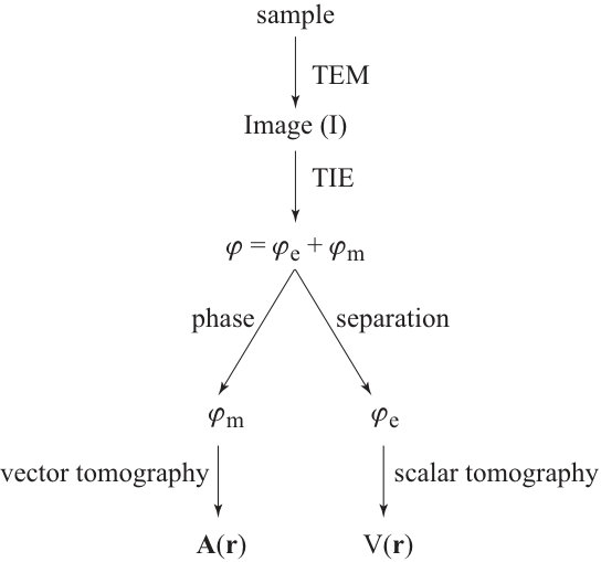 Figure 1
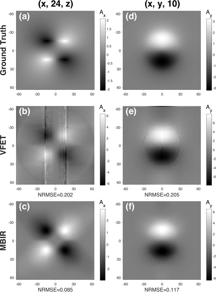 Figure 2
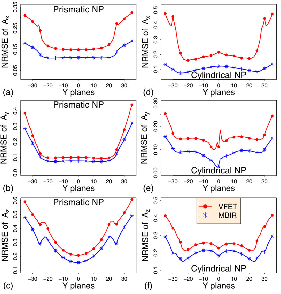 Figure 3
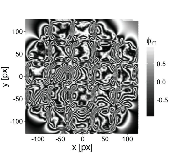 Figure 4
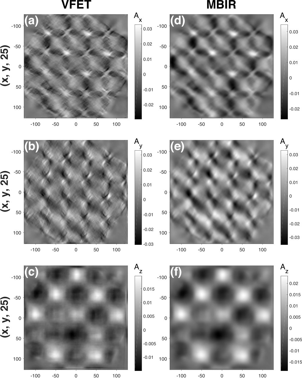 Figure 5
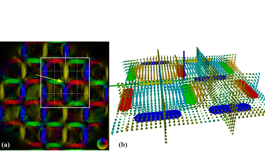 Figure 6
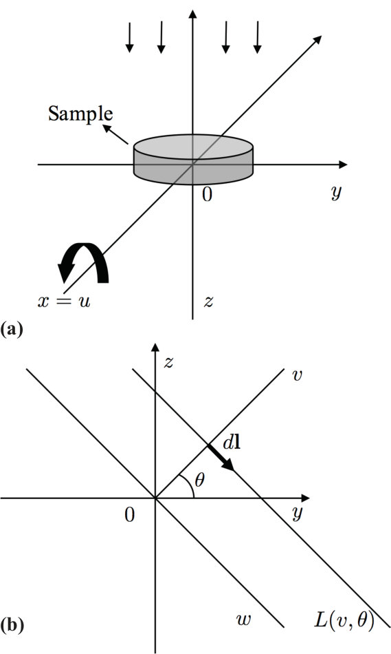 Figure 7
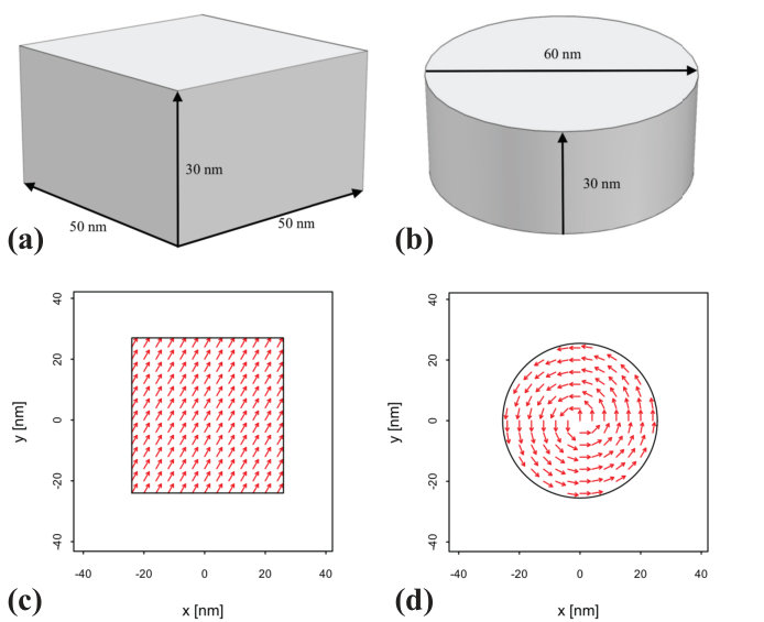 Figure 8
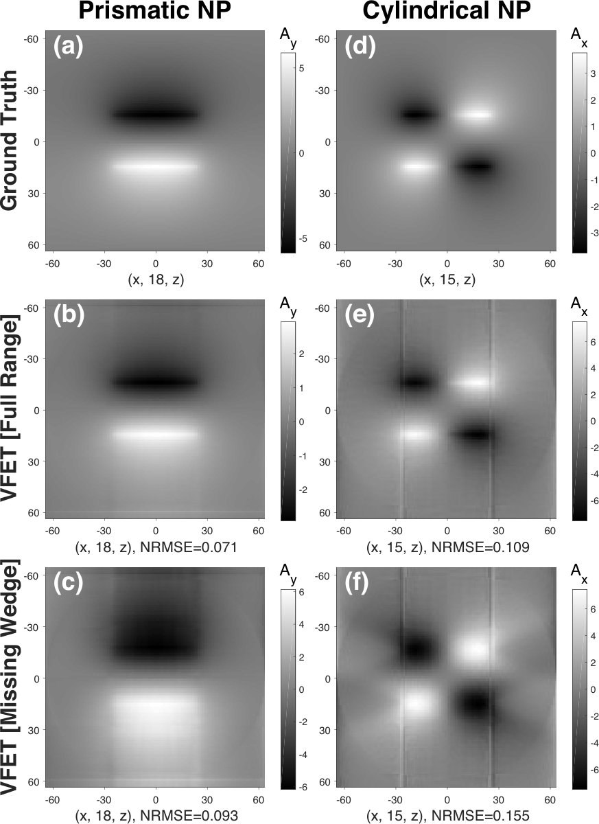 Figure 9
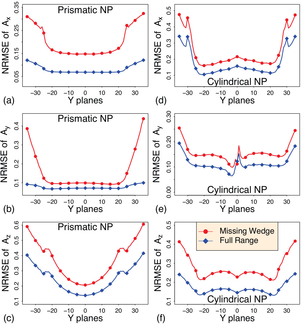 Figure 10
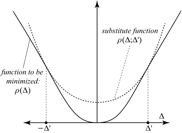 Figure 11
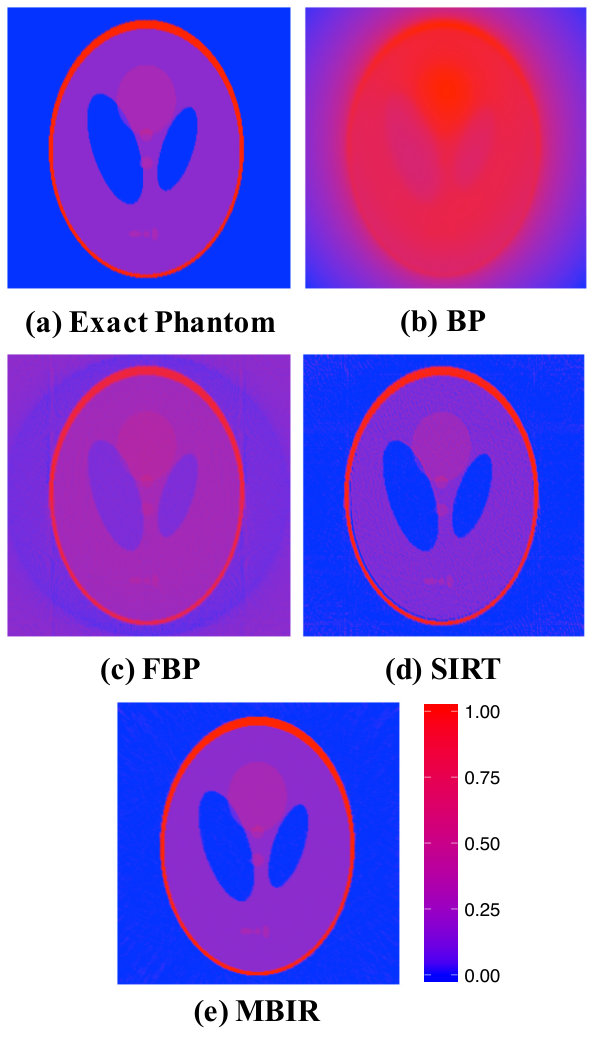 Figure 12
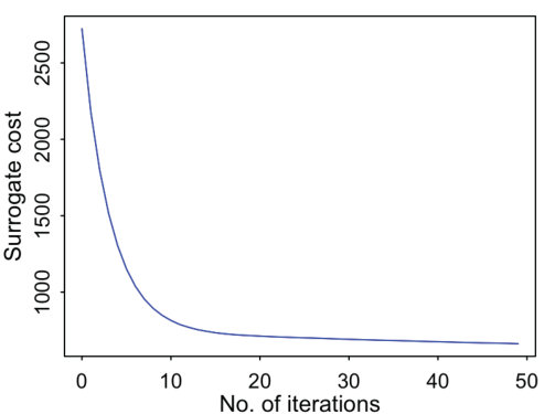 Figure 13
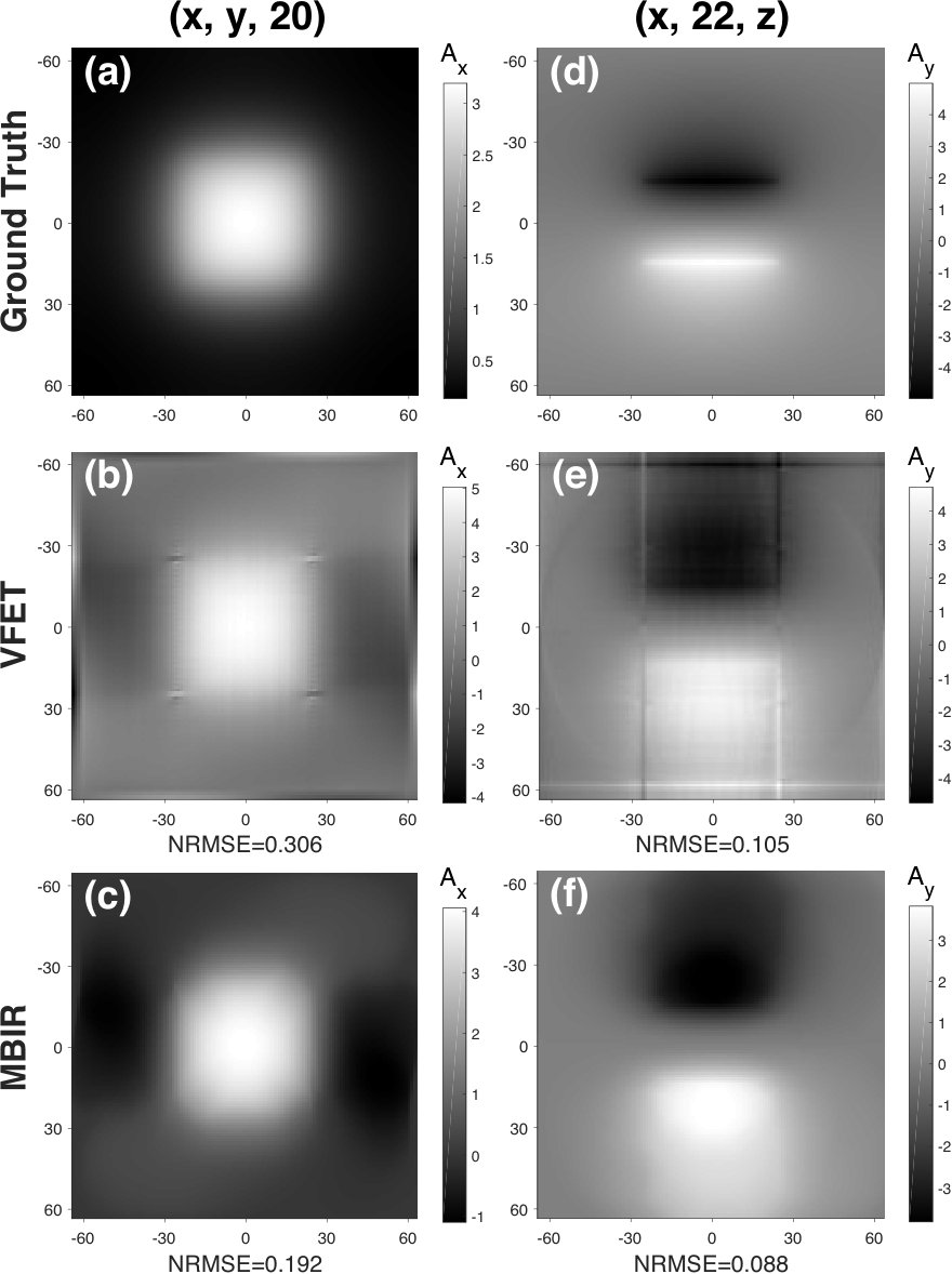 Figure 14
| Tomographic Method | RMSE |
|---|---|
| Back-Projection (BP) | |
| Filtered Back-Projection (FBP) | |
| Simultaneous Iterative Reconstruction Technique (SIRT) | |
| Model-Based Iterative Reconstruction (MBIR) |
Peer Reviews
No public reviews on file for this paper yet. If you reviewed it on a platform where reviews are public (OpenReview, ICLR, NeurIPS, ICML), you can paste yours below so the community can read it here.
Videos
No videos yet. Explain this paper in a talk, walkthrough, or lecture? Add one.
Taxonomy
TopicsElectron and X-Ray Spectroscopy Techniques · Advanced Electron Microscopy Techniques and Applications · Advanced X-ray Imaging Techniques
3D Reconstruction of the Magnetic Vector Potential using
Model Based Iterative Reconstruction
Prabhat KC
K. Aditya Mohan
Charudatta Phatak
Charles Bouman
Marc De Graef
Department of Materials Science and Engineering, Carnegie Mellon University, Pittsburgh, Pennsylvania, USA
Department of Electrical and Computer Engineering, Purdue University, West Lafayette, IN, USA
Argonne National Laboratory, Lemont, Illinois, USA
Abstract
Lorentz Transmission Electron Microscopy (TEM) observations of magnetic nanoparticles contain information on the magnetic and electrostatic potentials. Vector Field Electron Tomography (VFET) can be used to reconstruct electromagnetic potentials of the nanoparticles from their corresponding LTEM images. The VFET approach is based on the conventional filtered back projection approach to tomographic reconstructions and the availability of an incomplete set of measurements due to experimental limitations means that the reconstructed vector fields exhibit significant artifacts. In this paper, we outline a model-based iterative reconstruction (MBIR) algorithm to reconstruct the magnetic vector potential of magnetic nanoparticles. We combine a forward model for image formation in TEM experiments with a prior model to formulate the tomographic problem as a maximum a-posteriori probability estimation problem (MAP). The MAP cost function is minimized iteratively to determine the vector potential. A comparative reconstruction study of simulated as well as experimental data sets show that the MBIR approach yields quantifiably better reconstructions than the VFET approach.
keywords:
Lorentz microscopy; Phase shift; Vector Field Electron Tomography (VFET); Model Based Iterative Reconstruction (MBIR).
\DeclareCaptionType
algorithm
1 Introduction
In a Lorentz Transmission Electron Microscopy (LTEM) experiment, an electron propagating through a thin specimen experiences a Lorentz Force [1] due to the sample’s electrostatic field, , and magnetic field, ; is the electron’s charge and its velocity. This (classical) force generates a deflection of the electron trajectory, which can be used to explain the Fresnel and Foucault observation modes [2]. A more robust explanation of the nature of the electron-specimen interaction involves quantum mechanics, in which the electron is described by a wave function [2]. Elastic scattering in the sample produces variations of the amplitude , whereas the electromagnetic potentials affect the phase of the wave; is a vector normal to the propagation direction. Aharonov and Bohm [3] showed, in 1959, that the phase of the exit wave function encodes information on the sample’s electrostatic potential, , and magnetic vector potential, , as follows:
[TABLE]
where is the reduced Planck’s constant, is the total beam energy, and the integrals are carried out along the beam direction, . The total phase shift, , consists of an electrostatic contribution, , and a magnetic contribution, . The phases are not directly observable, but their effect on the image contrast can be determined by considering the point spread function, , of the Lorentz lens. The image intensity is then given by the modulus-squared of the convolution product [2]. Hence, characterization of the electromagnetic potentials begins with phase shift retrieval from the image intensities, using either electron holography [4] or the transport-of-intensity equation (TIE) formalism [5], which is based on a through-focus series of Fresnel images. We use the linearity of the TIE [6] and time reversal symmetry to retrieve the individual phases and .
Characterization of the electromagnetic fields is then achieved by performing scalar field and vector field tomographic reconstructions to determine and , respectively. We refer to the use of vector field tomography to reconstruct the electromagnetic potentials as Vector Field Electron Tomography (VFET) [7]. A schematic of the operations performed to complete an electromagnetic characterization task is shown in Fig. 1.
In this contribution, we primarily focus on vector field tomography to reconstruct . In recent years, the VFET approach employed the filtered back projection (FBP) approach to perform the reconstructions [8, 9]. Although FBP yields a good estimate with a complete set of measurements, the typical missing wedge of TEM data significantly diminishes the quality of the reconstructions [10]. In addition, typical tilt series are obtained using an angular step size of – to minimize the necessary pre-processing steps (image alignments) and reduce beam damage. These limitations, collectively, yield a reconstruction result that can exhibit substantial artifacts. To alleviate these problems, we resort to a more robust and statistically based tomographic reconstruction framework known as Model-Based Iterative Reconstruction (MBIR) to determine . This approach has had considerable success in improving reconstruction quality in scalar tomography [11, 12].
In section 2, we briefly outline conventional VFET and show how we can reconstruct all three component of from just two tilt series; we also perform an error analysis of the quality of VFET reconstructions in the presence of a missing wedge. Next, in section 3, we provide an overview of the MBIR framework, and in section 4, we incorporate MBIR into the reconstruction of and compare the results with those from conventional VFET reconstructions.
2 Vector Field Electron Tomography
Vector field tomography is relatively new; it was not until 1988 when Norton [13], for the first time, outlined a mathematical model to determine the 2D fluid field from acoustic time travel measurements. Subsequent years saw extensions of 2D vector tomography to 3D cases; in particular, Juhlin [14] resolved the solenoidal part of a divergence free flow field using ultrasound Doppler measurements in 1992. In 2005, Lade et al. [8] presented the VFET model to reconstruct 3D vector fields from longitudinal and transverse measurements. In 2008, Phatak et al. [15] used the VFET approach to reconstruct the magnetic vector potential and induction of magnetic nanoparticles. Since this VFET model is still relevant for our new MBIR method, we devote this section to a brief review of the VFET framework.
Since tomographic reconstructions require a forward model to project the object being reconstructed, we begin by considering the computation of the magnetic phase shift. The relation describes the magnetic phase shift obtained at tilt. To obtain the phase shift for a tilted sample we consider a tilt series around the axis (counterclockwise); the new coordinate vectors, can be expressed in terms of the original ones, by where , , and is the counter-clockwise rotation matrix (Fig. 2(a)). From Fig. 2(b), the vectorial line element, , of the projection line , can be written as .
Writing , a generic projection equation for the tilt series in Fourier space, , can be obtained as:
[TABLE]
a similar analysis for the tilt series produces
[TABLE]
Eqs. 2 and 3 represent the Fourier slice theorem for 3D vector fields for tilt series and tilt series respectively.
The formulation of the reconstruction procedure by means of the VFET approach begins by imposing a gauge constraint on the magnetic vector potential, i.e., . This constraint is written in Fourier space as:
[TABLE]
Combining eqs. 2, 3, and 4 and solving for the components of one obtains:
[TABLE]
In principle, one could interpolate the projection measurements from the polar grid to a Cartesian grid and perform an inverse Fourier transform (FT) to solve for . However, this is a numerically unstable approach and the filtered back projection formulae, as outlined in ref. [16], facilitate a more stable reconstruction. In the present case, the FBP formulae become (the asterisk subscript represents , , or ):
[TABLE]
where
[TABLE]
In eqs. 15 and 22, and represent the filtering operation and the 2D inverse FT. The real-space vector quantities and , are then used to determine the three components of through an inverse Hough transform. The gauge condition on will be incorporated into the MBIR approach as well. However, we will replace the FBP formula of eq. 8 with a Bayesian inference-based objective function which will be described in more detail in the next section.
Before we outline the MBIR framework, we illustrate the numerical implementation of the VFET approach using uniformly and non-uniformly magnetized simulated magnetic nanoparticles (MNPs); in particular, we use a uniformly magnetized prismatic particle and a circular disk with a vortex state. The prismatic nanoparticle (NP) has dimensions of nm and magnetization direction, . The circular disk has a diameter of nm, a height of nm, and exhibits a counterclock-wise magnetization state with a sharp vortex [17, 18]. Both particles have a saturation magnetization of T. The two geometries and their magnetization states are depicted in Fig. 3.
Starting from the magnetization states, the Fourier transform of the magnetic vector potential can be expressed in terms of the shape function formalism of Ref. [17] as:
[TABLE]
where is the shape amplitude. This expression allows for the computation of the magnetic phase shifts for two orthogonal tilt series around the and axes. In one series we use projections over the full tilt range with a step size while in a second series, with a missing wedge, we use the sub-range of . After application of the VFET approach described above we compare the reconstructed potentials with their corresponding known values (i.e., ground truths), in terms of a normalized root mean square error (NRMSE) between the reconstructed result, , and the ground truth, , as ( represents one of the components of the vector potential):
[TABLE]
Fig. 4 compares sections of reconstructed vector potentials with their ground truths, and lists the corresponding NRMSE values. Blurring at edges and ring artifacts are clearly more prominent in the reconstructions from the missing wedge data set, which has a higher NRMSE value than the reconstruction using the full tilt series. Fig. 5 shows the NRMSE values corresponding to the planes in the range . These plots indicate that the reconstruction deduced from the missing wedge data set exhibits a higher level of deviation from the ground truth than its full range counterpart by about –%. In the following section, we will replace the filter based analytical relation of eq. 8 with a Bayesian statistics-based numerical relation.
3 The MBIR framework
We introduce the MBIR approach by first formulating its framework for a generic tomography problem. Let be the discrete vector of an unknown image and be the discrete vector of projection measurements of at a variety of angles. Then the MBIR approach performs a reconstruction by maximizing the joint probability distribution resulting from the likelihood function, , and the prior distribution, . This methodology is more commonly known as the maximum-a-posteriori (MAP) estimation technique [19]. Mathematically, the MAP estimate is expressed as:
[TABLE]
We use the Poisson probability mass function to model the likelihood term. We use a second order Taylor series expansion of the logarithm of the Poisson distribution [20] to approximate the first term of eq. 25 as:
[TABLE]
where is the forward projection matrix, is a diagonal noise weighting matrix and is a term independent of the optimization variable . Additionally, is an orthogonal matrix such that ; hence, denotes the back projection operator.
The prior term in eq. 25 is modeled using a Markov Random Field (MRF) in:
[TABLE]
where denotes the set of neighboring pixels, is a non-causal symmetric weighing filter that is normalized such that , and is the potential function. The choice of the MRF as the prior model is due to its proven usefulness in image processing as well as in tomographic reconstructions [21, 22]. In the present paper, we resort to a class of MRFs called the -Generalized Gaussian Markov Random Field (-GGMRF) to model the prior. Accordingly, the potential function in eq. 27 is given by:
[TABLE]
where , and are the -GGMRF parameters. Typically, is used to ensure strict convexity of the potential function and, subsequently, of the MAP optimization [23]; in this paper we use . When is set to , the potential function is quadratic and the prior model facilitates a reconstruction with smooth edges. On the other hand, when is close to , the prior model performs sharp edge preserving reconstructions. Similarly, is the variance of the prior distribution and its value is set to achieve a balance between noise and resolution. Finally, the constant determines the approximate threshold of transition between low and high contrast regions.
Substituting the log-likelihood expression of eq. 26 and the prior model of eq. 27 into eq. 25, and considering as the identity matrix, one obtains the MAP reconstruction to be the solution of the following optimization problem:
[TABLE]
where the cost (objective) function being minimized is given by
[TABLE]
Before proceeding with the minimization of the cost function, it should be noted that differentiating the cost function with respect to and setting the derivative to zero does not yield a closed form solution. Accordingly, one needs to make use of numerical methods, e.g., the Newton-Raphson method or the line search method, to determine the MAP estimate [20, 24]. However, these numerical methods can be computationally expensive to implement. Thus, we introduce the substitute or surrogate function to derive a closed form solution of the MAP estimate and subsequently facilitate a faster implementation [25]. A visual depiction of the intuition behind the substitute function is shown in Fig. 6. In accordance to the figure, symmetric bond method is employed to construct a substitute function, , as an upper bound to the original function, , such that minimizing the substitute function results in a lower value of the original function [26]. Accordingly, the potential function in eq. 27 is upper bounded by a symmetric and quadratic function of . Then its substitute form can be expressed as:
[TABLE]
where is a function of . Here, is determined by matching the gradient of and at to yield:
[TABLE]
Substituting the value of in eq. 31 results in the following symmetric bound substitute function:
[TABLE]
where the limiting value of is used when . Subsequently, we obtain the new MAP cost function as:
[TABLE]
where
[TABLE]
The surrogate cost function in eq. 34 is quadratic and so its minimum can be expressed in closed form. We use the Iterative Coordinate Descent (ICD) method to numerically minimize the surrogate cost function [25]. ICD works by sequentially minimizing the cost function of eq. 34 with respect to each pixel. The convergence of the ICD technique to solve the optimization problem can be inferred from the fact that the surrogate cost function in eq. 34 is strictly convex so that any locally optimal point is also globally optimal. Thus, we proceed to differentiate the surrogate cost function and solve for the minimum to yield each pixel update as:
[TABLE]
{algorithm}
[t]
1:initialize
2:
3:while not converged do
4: for to do
5: \text{for }\{i,j\}\in\mathcal{C}\text{ of }u_{i}\text{ determine }\tilde{b}_{ij}\text{ using eq.\leavevmode\nobreak\ \ref{eq:tilde_bij_val}}
6:
7: end for
8:
9:
10:end while
Fourier Transform-based MBIR method for scalar tomography
A pseudocode to minimize the surrogate cost function for a pixel wise update using the ICD technique is listed in Algorithm 3. Note that, in contrast to the widely observed MBIR practice of updating the error sinogram, , after each pixel update, we resort, instead, to updating after all pixels have been modified. This is primarily due to the fact that we will be using a Fourier-based forward model instead of a Radon based forward model [12] to minimize the cost function. The Fourier-based forward model is chosen to make the framework compatible with imposing a Coulomb gauge constraint when we extend it for the reconstruction of .
We conclude this section with the implementation of the MBIR methodology to a 2D scalar tomography problem. We make use of the standard Shepp-Logan head phantom [27] to illustrate our results. The phantom or ground truth is depicted in Fig. 7(a); it is pixels in size and has values ranging from [math] to , which we map on a blue-red color scale. In addition to the result from the MBIR approach (Fig. 7(e)), we also show results from other reconstruction techniques, such as back projection (BP) in Fig. 7(b) and FBP in Fig. 7(c). We used a band-limited Ram-Lak ramp filter as our filtering function [28, 29]. The result from an implementation of a conventional iterative tomography method known as the Simultaneous Iterative Reconstruction Technique (SIRT) is shown in Fig. 7(d).
Table 1 lists the root mean square error (RMSE) between the reconstructed results, , and the true phantom, , for several tomographic reconstruction methods. Mathematically, the RMSE is expressed as:
[TABLE]
The RMSE value of the BP result was ; such a high RMSE value was expected as the BP method is the simplest form of reconstruction technique and does not incorporate any filter or iterative technique in its model. The RMSE value decreases to about for the FBP approach. Reconstruction by the SIRT method shows further improvement as the ring artifact, seen in the FBP result, is entirely eliminated, resulting in an RMSE value of . The effectiveness of the SIRT approach over analytical method like the FBP approach stems from the fact that the SIRT algorithm iteratively minimize the error sinogram as [30]:
[TABLE]
where is a relaxation parameter. However, the ill-posed nature of the tomography problem limits the SIRT strategy to exhibit only semi-convergence [30, 31]. Accordingly, improvements seen in the first few SIRT iterations start to deteriorate as the number of iterations increases due to noise propagation. In our analysis, we show a locally converged SIRT result obtained after iterations with and set as the identity matrix.
The MBIR reconstruction is obtained by iteratively minimizing the surrogate cost function of eq. 34 which, in turn, is achieved by following Algorithm 3. The -GGMRF parameters used in this implementation were . We used a non-causal weighting matrix, , to incorporate the influence of two nearest neighbors for any given pixel. The first nearest neighbors are weighted by a factor of while the second nearest nearest neighbors are weighted by a factor of . The decreasing trend of the surrogate cost function over several iterations is shown in Fig. 8. An important point to note here is that the decreasing trend of the surrogate cost is a direct consequence of its strictly convex nature. Convergence after the cost minimization means that the reconstruction is globally minimal and unique. Hence, the coarseness seen along the inner region of the locally converged SIRT result is no longer visible in the MBIR result. Also, the superiority of the MBIR approach over any of the other tomography methods can be discerned from the RMSE analysis which reveals an error of only .
4 MBIR-based vector field reconstruction
The MBIR framework for vector field reconstruction revolves around solving an optimization problem similar in form to the one expressed in eq. 25. Specifically, we seek to formulate a framework that will iteratively work to minimize the sum of the squared differences between the data and its estimated forward projection, in combination with a regularizing prior function, . However, in contrast to scalar tomography, vector reconstruction entails measurements from more than one tilt series; each tilt series involves a contribution from different components of . We also impose a gauge constraint to reconstruct all three components of vector potential from just two tilt series. Accordingly, our generic MBIR framework from section 3 needs to be expanded to account for input measurements from two tilt series and imposition of a gauge constraint.
We begin MBIR based vector reconstruction by representing the input data by , and subsequent estimates of the magnetic vector potential by . Let where and are operators for the forward projection of the magnetic vector potential for the and tilt series (counter-clockwise), in accordance with eqs. 2 and 3, respectively. Then the forward projection of yields, . We define a deconvolution operator, , which will serve to evaluate the contributions of the magnetic phase shift (eqs. 15 and 22) to each component of vector potential separately. Thus any of the components of the deconvolution operator, when applied to the phase shift, yields ; and its application to yields .
Next, we define the prior model analogous to the one defined in section 2. We use a -GGMRF as the potential function that minimizes the cost function for a given voxel based on the difference with its neighboring voxels. However, contrary to the 2D MBIR approach, we incorporate the influence of three nearest neighbors for any given voxel while evaluating the potential function . Accordingly, the non-causal weighting matrix, , now contains values with first, second and third weighing factors assigned as, , , and , respectively. Finally, we again make use of the surrogate majorization technique such that the -GGMRF potential function assumes a quadratic form for .
Having defined all the pertinent variables, we can now express MBIR-based vector reconstruction as the solution to the following optimization problem:
[TABLE]
where is determined using eq. 35. In practice, we do not directly solve eq. 39. Instead, we make use of the deconvolution operator, , and de-convolve eq. 39 into three MAP estimation problems as follows:
[TABLE]
Next, we identify the cost function associated with each of the potential estimates in eqs. 40, 41, and 42. For instance, the surrogate cost associated with the MAP estimate of is expressed as:
[TABLE]
Then we use the ICD algorithm, as detailed in section 3, to minimize the surrogate cost function of eq. 43. Differentiating eq. 43 with respect to and setting the result equal to zero, we obtain:
[TABLE]
In a similar manner, we solve for minimum corresponding to surrogate the cost functions of and in eqs. 41 and 42 to obtain:
[TABLE]
{algorithm}
[t]
1:Evaluate
2:
3:while not converged do
4: for to do
5: Determine corresponding for of using eq. 35
6:
7: end for
8: Update in a similar manner similar
9: Forward project using eqs. 2 and 3 to determine and , respectively
10: Determine the error sinogram for the two series as:
[TABLE]
11: Use the results of imposing gauge constraint from eqs. 15 and 22 on and to determine and
12: Update the components of the vector potential as
[TABLE]
13:end while
MBIR method to reconstruct magnetic vector potential
Note that the MAP estimate of each component of the vector potential, , is determined by performing element-wise minimization of its associated cost function from eqs. 40-42 with respect to the overall magnetic vector potential, , instead of the individual component, . This is primarily due to the fact that each component is reconstructed with the aid of two tilt series, , which in turn have contributions from all three components of the vector potential, . Hence, each ICD iteration consists of simultaneously evaluating eq. 44-46 and then making use of the forward model and the deconvolution operator to update the estimates of the vector component as:
[TABLE]
A summary of the MBIR-based reconstruction is illustrated in the form of pseudo code in Algorithm 4. In the next two subsections we make use of this MBIR algorithm to reconstruct the magnetic vector potential of synthetic as well as experimental data sets.
4.1 Synthetic Data Set
In this section, we apply the MBIR algorithm to the reconstruction of for the cylindrical and prismatic MNPs discussed in section 2. The reconstruction was performed making use of the missing wedge projection set since this set replicates the limited angular scenario typical of TEM based experimental measurements. The -GGMRF parameters used for the reconstruction comprised of . Selected results retrieved from the MBIR approach are depicted in Figs. 9 and 10. These figures also include corresponding plots from the ground truth and the VFET approach for the purpose of qualitative comparison of reconstruction accuracy between the two approaches. We also present a quantitative comparison between the two methods in terms of NRMSE plots in Fig. 11.
A review of the plots in Figs. 4, 9, and 10 reveals that the low spatial resolutions, protrusions, ring artifacts and edge artifacts evident in the VFET reconstructions are significantly suppressed in the MBIR-based reconstructions. In case of the prismatic MNP, we note that the MBIR-based reconstruction displays values in closer proximity to the ground truth than the ones obtained from the VFET reconstructions, as shown in Figs. 9(a-c). This is confirmed by the NRMSE plots in Figs. 11a and 11c which show that the MBIR approach determines and with to less planar error (in axis) than those derived from the VFET approach. On planes, such as , shown in Figs. 4(a-c), where the reconstructed vector potential suffers from strong edge artifact as a direct consequence of the limited angular range of projection measurement, the MBIR reconstruction performs significantly better than the VFET approach. In Fig. 9f, we observe that, although MBIR suppresses the ring artifact, the blurred edges persist; the loss of information due to the missing wedge is such that even an advanced algorithm as MBIR is unable to completely remove the artifacts observed in the VFET based reconstruction. This conclusion is also substantiated by the NRMSE plot in Fig. 11b which reveals that the gain in reconstruction accuracy having adopted the MBIR approach is merely to compared to the VFET approach.
For the cylindrical MNP, we see that the MBIR approach preserves the spatial resolution and retrieves vector potential values in closer proximity to the ground truth than the VFET approach, as depicted in Figs. 10(d-f). Accordingly, the NRMSE for planes of all three components of are less by about for MBIR reconstructions as compared to VFET reconstructions, as illustrated in Figs. 11(d-f). Also, edge and ring artifacts observed in the VFET reconstruction are substantially diminished in the MBIR reconstruction, as shown in Fig. 10(a-c). However, both MBIR and VFET results exhibit protrusion effects due to the missing wedge.
4.2 Experimental Data Set
In this final section we make use of a real data set to demonstrate the gain in reconstruction quality from making use of the MBIR approach. A 2D lattice of elongated (permalloy/py) islands (“stadia”) was used for the comparative study of the MBIR and VFET techniques. The sample was fabricated on a JEOL electron beam lithography system. A single layer of ZEP resist of nm thickness was coated on a Si/SiN substrate, followed by patterning of a square lattice with element shape parameters of nm, nm, and a lattice spacing of nm. A Py film of nm thickness was deposited on a seed layer of Cr ( nm) using dc magnetron sputtering at mTorr pressure and W power. The pattern was transferred by a lift-off process. This was followed by optical lithography and wet-etching of Si to create electron transparent windows on mm square grids, which could be loaded directly into the TEM for observation. The microscopy was performed using the JEOL 2100F TEM equipped with a dedicated Lorentz lens and a spherical aberration corrector [32].
The projection measurements acquired for tomographic reconstruction consist of and tilt series with angles ranging from to at a step size of . Fig. 12 depicts one of the projections as a holographic plot, , of the magnetic phase shift of the sample at tilt. Each phase map has a resolution of pixels ( nm per pixel). We implemented our tomographic reconstruction on a 3D voxel grid with nodes. First, we employed the VFET approach (as discussed in section 2) to determine an estimate of of the Py sample. These results are then used to initialize the MBIR algorithm. The -GGMFR parameters used in the MBIR algorithm are , , , and . The cost function in eq. 39 was then monotonically decreased over iterations to determine a MAP estimate of of the Py sample. The forward model calculation for each iteration was distributed over parallel threads using OpenMP and required about minutes to complete the iteration. Some of the results obtained from the VFET and MBIR approaches are depicted in Fig. 13.
A comparison of the plots deduced from the two methods reveals that the MBIR results show a significant gain in spatial resolution. The coarseness of the VFET result is substantially reduced in the MBIR result. Moreover, we see appropriately segmented and smoothly transitioning values in the MBIR results. The blurring artifacts observed in some of the VFET reconstruction sections are considerably diminished in the MBIR results. These reconstruction gains in the MBIR-based results are observed throughout the 3D spatial region when compared to their VFET counterparts.
Since the reconstructed quantity is a 3D vector field, we conclude this section with a 3D rendering (Fig. 14) of the magnetic vector potential resulting from the MBIR reconstruction approach. Fig. 14(a) shows a color-coded integrated (along the beam direction) magnetic induction map, derived from the magnetic phase shift by a gradient operation. The white rectangle delineates the region used for the 3D rendering of the vector field in Fig. 14(b). To reduce the complexity of the 3D rendering, the field vectors (shown as small cones with the appropriate orientation) are only drawn for the horizontal center plane going through the Py islands and four vertical planes corresponding to the dashed lines in Fig. 14(a). The yellow arrow indicates the viewing direction for the 3D rendering in Fig. 14(b). The individual islands are colored according to the in-plane direction of the integrated magnetic induction following the color wheel in (a). Note that the induction directions, which are oriented along the local curl of the magnetic vector potential, are properly oriented; i.e., the opposite rotation of the vector field around the green and red islands is clearly visible, and application of the right-hand rule for the curl results in the correct direction of the integrated magnetic induction. Furthermore, the square of islands on the left front of the image, and the two squares in the back, are all in a vortex state, i.e., the magnetization of the islands circulates clockwise or counterclockwise. The corresponding section through the vector field shows vectors which are all blue ( pointing down) or all orange ( pointing up). For the square on the front right, however, two of the islands are blue, so that there is no closed vortex and the vector field is much more complex in this area, reflecting the local frustrated state of the magnetization pattern.
5 Conclusion
In this contribution, we have incorporated the Bayesian inference-based MBIR technique into the tomographic reconstruction process for the 3D magnetic vector potential. The MBIR model is formulated by combining a vector slice-based forward model and a -GGMRF-based prior model. An objective function was constructed and minimized using the Iterative Coordinate Descent technique to determine a MAP estimate of . The MAP estimate shows diminished edge, ring and blurring artifacts when directly compared to reconstructions carried out with the more traditional filtered back-projection reconstruction from the VFET methodology. This qualitative conclusion is confirmed by the NRMSE values for simulated magnetic nan-particles with uniform as well as non-uniform magnetization configurations and prismatic and cylindrical particle shapes. We have implemented the MBIR technique to reconstruct the magnetic vector potential of a 2D array of Py islands. The resulting vector field was compared to an integrated magnetic induction map derived from the magnetic phase shift and is in good agreement.
Acknowledgements
PK and MDG acknowledge financial support from a U.S. DOE grant (DE-FG02-01ER45893) which supported the development of the 2D MBIR approach, and an NSF grant (DMR #1306296), which supported the final development of the 3D MBIR reconstructions. AM and CB acknowledge an AFOSR MURI grant # FA9550-12-1-0458 for financial support. The experimental work by CP was supported by the U.S. Department of Energy, Office of Science, Basic Energy Sciences, Materials Sciences and Engineering Division. Use of Center for Nanoscale Materials was supported by the U.S. Department of Energy, Office of Science, Office of Basic Energy Sciences, under contract no. DE-AC02-06CH11357. The authors would also like to acknowledge the computational facilities of the Materials Characterization Facility at CMU under grant # MCF-677785.
The reference list from the paper itself. Each links out to its DOI / PubMed record.
- 1[1] J. Jackson, Classical Electrodynamics, second ed., Wiley, NY, 1975.
- 2[2] M. De Graef, Lorentz Microscopy: Theoretical Basis and Image Simulations, M. D. Graef, and Y. Zhu (Eds.), Magnetic Imaging and Its Applications to Materials, Vol. 36, Academic Press, San Diego, CA, 2001 (Chapter 2).
- 3[3] Y. Aharonov, D. Bohm, Significance of electromagnetic potentials in the quantum theory, The Phys. Rev. 115 (1959) 485–491.
- 4[4] P. A. Midgley, R. E. Dunin-Borkowski, Electron tomography and holography in materials science, Nature Materials 8 (1997) 271–280.
- 5[5] D. Paganin, K. A. Nugent, Noninterferometric phase imaging with partially coherent light, Phys. Rev. Lett. 80 (1998) 2586–2589.
- 6[6] E. Humphrey, C. Phatak, A. Petford-Long, M. De Graef, Separation of electrostatic and magnetic phase shits using a modified transport-of-intensity equation, Ultramicroscopy 139 (2014) 5–12.
- 7[7] Z. Kemp, T. Petersen, D. Paganin, K. Spiers, M. Weyland, M. Morgan, Analysis of noise-induced errors in vector-field electron tomography, Phys. Rev. A 90 (2014) 023859.
- 8[8] S. Lade, D. Paganin, M. Morgan, 3-D Vector tomography of doppler-transformed fields by filtered-backprojection, Opt. Commun. (2005) 382–391.