Dynamics of a family of continued fraction maps
Muhammed Uluda\u{g}, Hakan Ayral

TL;DR
This paper investigates a family of continued fraction maps, including the Gauss and Fibonacci maps, analyzing their transfer operators, invariant measures, and a related involution, revealing common functional equations and specific invariant measures.
Contribution
It introduces a unified framework for analyzing a family of continued fraction maps, deriving their transfer operators and invariant measures, and exploring their interrelations through an involution.
Findings
Invariant measures satisfy a common functional equation.
Explicit invariant measures found for some family members.
An involution relates the Gauss and Fibonacci maps.
Abstract
We study the dynamics of a family of continued fraction maps parametrized by the unit interval. This family contains as special instances the Gauss continued fraction map and the Fibonacci map. We determine the transfer operators of these dynamical maps and make a preliminary study of them. We show that their analytic invariant measures obeys a common functional equation generalizing Lewis' functional equation and we find invariant measures for some members of the family. We also discuss a certain involution of this family which sends the Gauss map to the Fibonacci map.
Click any figure to enlarge with its caption.
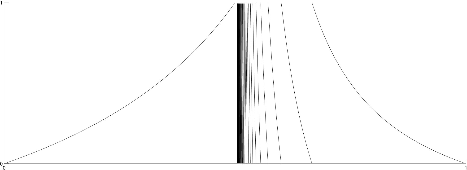 Figure 1
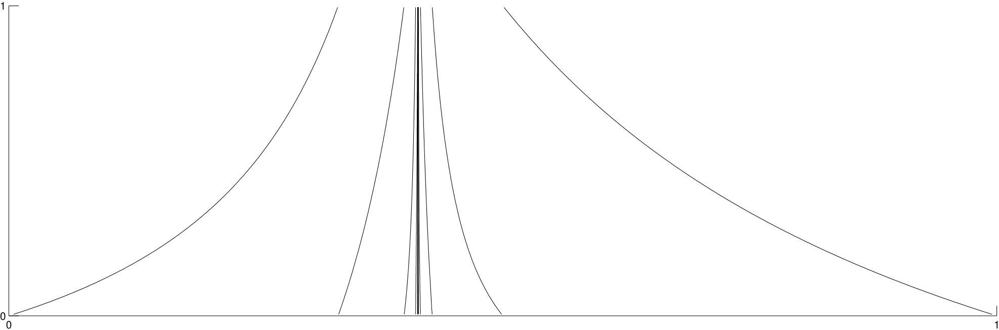 Figure 2
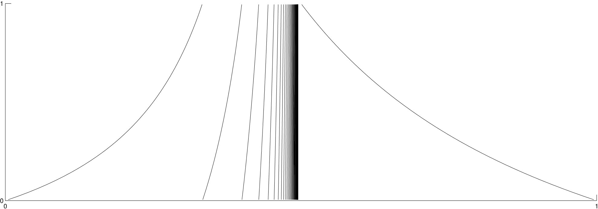 Figure 3
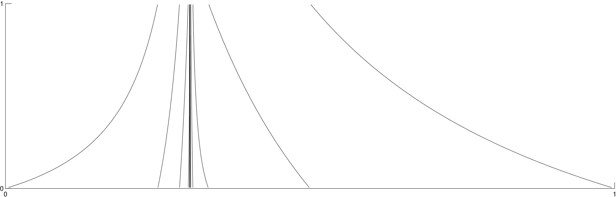 Figure 4
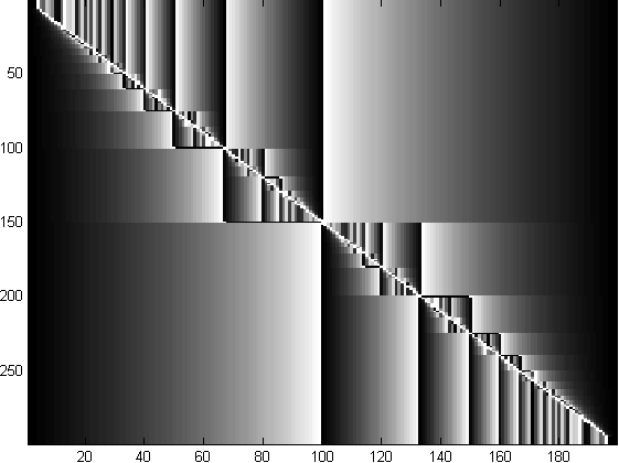 Figure 5
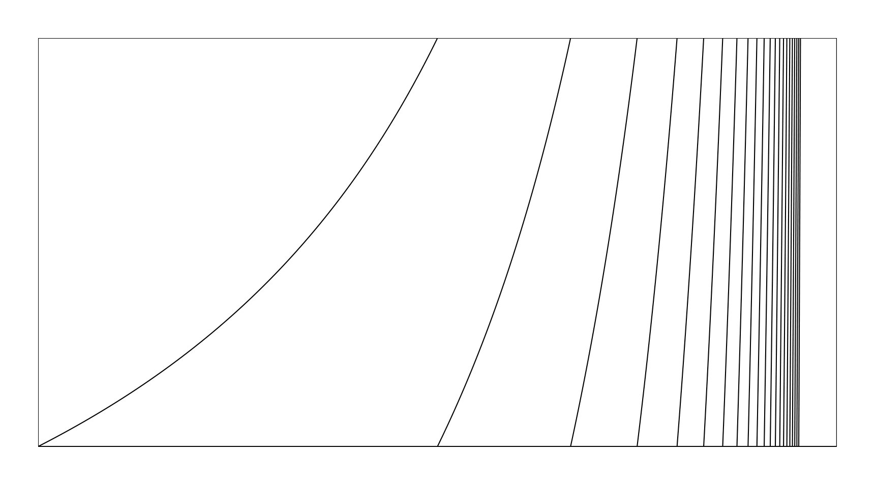 Figure 6
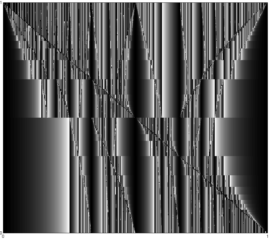 Figure 7
 Figure 8
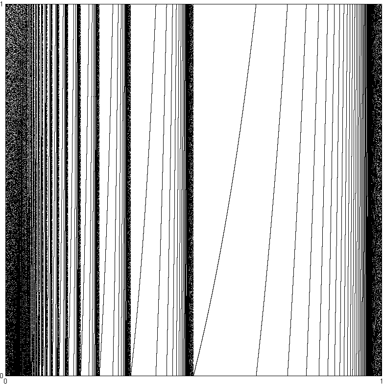 Figure 9
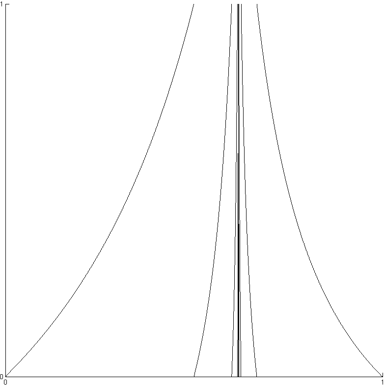 Figure 10
 Figure 11
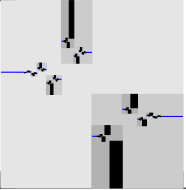 Figure 12
Peer Reviews
No public reviews on file for this paper yet. If you reviewed it on a platform where reviews are public (OpenReview, ICLR, NeurIPS, ICML), you can paste yours below so the community can read it here.
Videos
No videos yet. Explain this paper in a talk, walkthrough, or lecture? Add one.
Taxonomy
TopicsMathematical Dynamics and Fractals · Quantum chaos and dynamical systems · Advanced Differential Equations and Dynamical Systems
Dynamics of a family of continued fraction maps
Muhammed Uludağ∗, Hakan Ayral111 Department of Mathematics, Galatasaray University Çırağan Cad. No. 36, 34357 Beşiktaş İstanbul, Turkey
Abstract
We study the dynamics of a family of continued fraction maps parametrized by the unit interval. This family contains as special instances the Gauss continued fraction map and the Fibonacci map. We determine the transfer operators of these dynamical maps and make a preliminary study of them. We show that their analytic invariant measures obeys a common functional equation generalizing Lewis’ functional equation and we find invariant measures for some members of the family. We also discuss a certain involution of this family which sends the Gauss map to the Fibonacci map.
1 Introduction
Denote the continued fractions in the usual way
[TABLE]
where are integers. Our aim in this paper is to study a family of continued fraction maps , parametrized by and defined as
[TABLE]
where and
Plot of the map as a function of and . The intensity is proportional to the value of . The symmetry reflects the fact that .
The first thing to notice about this family is that it is not continuous in the variable , the two representations of rational as a continued fraction leads to two different maps with distinct dynamical behaviors. Another problem is that is not defined if or if with one of its two continued fraction expansions being an initial segment of . We overcome this issue by assuming that the rational are represented by continued fractions with . Consequently, we set for such . We also set .
Each constitutes a Möbius system [10] which is a special kind of a fibered system [11]. For , the map is the Gauss continued fraction map [3], [2] and for , is the so-called Fibonacci map [4]. In Section 3 below we recall some basic facts about them and prove that they are in fact conjugates of each other. In the preceding Section 2, we define a transfer operator for and prove that their invariant functions obeys a common functional equation generalizing Lewis’s. Section 4 is devoted to the study of some other special instances of the family . In particular for () we determine an analytic invariant measure for .
2 Transfer operators and functional equations
To give another perspective on , first represent by a binary string (always starting with a ) with for all . Also represent in this form. Then compares the strings of and and returns with the initial segment matching with that of chopped off. If the remaining sequence starts with a , then it permutes [math]’s with ’s.222Alternatively, one may assume that and represents the same continued fraction.
2.1 The transfer operator
To write a transfer operator for , note that its inverse branches are
[TABLE]
Set for the Koopman operator. Its left-adjoint with respect to its action on the set of cumulative distribution functions of probability measures on is the “integral” Gauss-Kuzmin-Wirsing operator
[TABLE]
Assuming is differentiable and the convergence is nice, we may take derivatives which yields the operator
[TABLE]
We will call this the Gauss-Kuzmin-Wirsing (GKW) operator of .
To handle the alternation of signs, set
[TABLE]
where and . Then
[TABLE]
Now we define the transfer operator as below, which specializes to the Gauss-Kuzmin-Wirsing operator when :
[TABLE]
We will consider as a real variable and use the following practical form for :
[TABLE]
The first summand can be written as
[TABLE]
where for rational , the terms in (2) vanish.333We stress that for rational the two different choices for the continued fraction representation of will lead to two different dynamical maps and transfer operators. We will discuss these below. Hence
[TABLE]
A natural domain for is the space of functions of bounded variation on the interval . The first term in (3) apparently violates this and requires that to be defined on a larger domain. However, this term serves only to counterbalance its identical twin hidden in the infinite summand in (3).
Consider the action of on the set of functions on defined by
[TABLE]
Set and . Then
[TABLE]
and one may write
[TABLE]
Alternatively,
[TABLE]
Now one has, using the form (4) above,
[TABLE]
Hence =
[TABLE]
and therefore
[TABLE]
Summing the last two equations we get
[TABLE]
Now suppose that is an eigenfunction with eigenvalue , i.e. . Then
[TABLE]
Observe that is precisely Lewis’ three-term functional equation and is Isola’s transfer operator of the Farey map. Written explicitly, this equation looks as follows:
[TABLE]
It is readily seen in the explicit form that any 1-periodic odd function solves Equation 10. The set of all solutions forms a vector space over . Note that, for a given solution of Equation 10, the infinite series defining may or may not converge; even if it does, may or may not be an eigenfunction of . See [6] for a study of the case .
For , one may regroup (10) in several interesting ways. For example,
[TABLE]
Setting
[TABLE]
we arrive at the cocycle relation
[TABLE]
In order to solve the equation for , we need an inverse for the operator . To be more explicit, this is the operator
[TABLE]
Its kernel equation is precisely the functional equation for analytic eigenfunctions of Mayer’s transfer operator; and specialize to the following three-term functional equation when .
[TABLE]
This functional equation is connected to the one studied by Lewis and Zagier [6]. Modulo the above remark about its kernel, one can formally invert the equation and write
[TABLE]
Now if then since , the above inversion formula becomes simply . Taking into account the kernel of , we may write
[TABLE]
where is a solution of (16) and satisfies . Note that
[TABLE]
Another rearrangement of Equation 10, which makes explicit the connection with Lewis’ functional equation, is
[TABLE]
Setting gives again the cocycle relation The equation (i.e. the case ) is precisely the following three-term functional equation studied by Lewis and Zagier [6]:
[TABLE]
2.2 Common invariant measure
The maps share a common invariant measure, namely Minkowski’s measure, whose cumulative distribution function is given as
[TABLE]
Actually, ? is the common invariant measure of a much wider class of maps whose inverse branches are all on . To see the this, suppose that the inverse branches of are . Then each can be written as
[TABLE]
where and depends on . Suppose is a random variable on the unit interval with law ? and set . The law of is
[TABLE]
and the series of the last line must sum up to 1, because and are both probability laws.
3 Gauss and Fibonacci maps
In this section, we will discuss the two special instances of the family , namely the Gauss map and the Fibonacci map , where .
3.1 The Gauss map
If with , then in the definition (1) of we are always in the first case , and so is the well-known Gauss continued fraction map
[TABLE]
where and denotes the fractional part of . One has
[TABLE]
Its invariant functions are solutions of the functional equation
[TABLE]
Substituting in place of leads to the three-term functional equation
[TABLE]
which admits, when the function (called the Gauss density)
[TABLE]
as a solution. It is well known and easily verified that the Gauss density is an invariant density for the classical GKW-operator .
Mayer [7] considered the operator as acting on the space of functions holomorphic on the disc and proved that the determinant of exists in the Fredholm sense and equals to the Selberg zeta function of the extended modular group.
3.2 The Fibonacci map
If , then in the definition (1) of we are always in the first case , so that is the Fibonacci map
[TABLE]
where denotes the string which consists of consecutive 1’s and it is assumed that and . This map was introduced in [4] and studied in [1] from a dynamical point of view.
In our subsequent paper [12] we also announced some similar and complementary results. In the next section we show that and are in fact conjugates, albeit via a discontinuous involution of the real line induced by the outer automorphism of the extended modular group , studied in [12].
The map have the invariant measure and gives rise to a transfer operator ( denotes the th Fibonacci number)
[TABLE]
analytic eigenfunctions of which satisfies the three-term functional equation
[TABLE]
for the eigenvalue .
The Gauss map is sometimes described as an acceleration (induction) of the Farey map. One may view as another acceleration of the Farey map.
3.3 Conjugating the Gauss map to the Fibonacci map
The Fibonacci map is the conjugate of the Gauss map under an involution.
To recall its definition from [12], for with , one has
[TABLE]
where denotes the sequence of length , and the resulting ’s are eliminated in accordance with the rules and . Using the shift description of and the continued fraction description of the involution , we see that
[TABLE]
The Fibonacci map has infinitely many fixed points, which are
[TABLE]
with Note that with . The points are exactly the fixed points of the Gauss map. More generally, gives a correspondence between the periodic orbits of the Gauss map and those of the map :
[TABLE]
Hence, is -periodic orbit for if and only if is -periodic for .
Finally, note that the following functional equation is satisfied:
[TABLE]
For , this specialises to .
3.4 Lyapunov exponents
The Lyapunov exponent of a map is defined as
[TABLE]
The function is –invariant. For the Gauss map , the Lyapunov exponent is given by
[TABLE]
with the successive denominators of the continued fraction expansion. By Khintchin’s theorem [5] this limit equals for almost all . It is known that (see [9]), if the asymptotic proportion of 1’s among the partial quotients of equals 1, then the Lyapunov exponent of (with respect to the Gauss map) is . Now since for almost all , the asymptotic proportion of 1’s among the partial quotients of equals 1, we know that for almost all . It follows that, for almost all
[TABLE]
[TABLE]
[TABLE]
[TABLE]
[TABLE]
[TABLE]
[TABLE]
Now there is a bad possibility. The expression inside the brackets is convergent, so it may tend to 0. However this happens only when
[TABLE]
Hence, the Lyapunov exponent of the Fibonacci map is, for almost all .
[TABLE]
again, but for a different reason then the equality for almost all .
The Lyapunov spectrum of a map is defined as the level sets of the Lyapunov exponent , by . These sets provide a –invariant decomposition of the unit interval, We don’t have a handy description of the Lyapunov spectrum of the map .
3.5 Zeta functions
Since is the Hurwitz zeta , values of the transfer operator at the power functions can be viewed as analogues of the Hurwitz zeta:
[TABLE]
In particular,
[TABLE]
reducing to a two-variable Fibonacci-Hurwitz-zeta for
[TABLE]
and further reducing to the Fibonacci zeta when :
[TABLE]
It is known that the Fibonacci zeta admits a meromorphic continuation to the entire complex plane and its values at negative integers lies in the field (see [8] and references therein). The three-variable zeta satisfies the functional equation
[TABLE]
which is analogous to the functional equation of the Hurwitz zeta: .
4 Dynamics of for some special -values.
Double representation for rationals leads to two different ’s at those points. Recall that for , the two different continued fraction representations of gives rise to two distinct dynamical maps. We shall denote these when the continued fraction of ends with and otherwise.
Now, let us discuss some special members of this family of dynamical maps.
4.1 The map :
Here we have . One has
[TABLE]
Graph of the map .
One has
[TABLE]
For and we get
[TABLE]
So, is an invariant measure. For the image of the constant function we get the Hurwitz zeta function:
[TABLE]
We may express the operator in terms of the Mayer transfer operator as
[TABLE]
where . In other words, is an eigenfunction for if and only if is an eigenfunction for with the same eigenvalue.
4.2 The map :
Here we have or .
[TABLE]
[TABLE]
These two operators are equivalent under the transformation
[TABLE]
For the image of the constant function we get:
[TABLE]
For a fixed function of the operator one has
[TABLE]
Hence, fixed points of the operator satisfies the functional equation
[TABLE]
In virtue of the equivalence (24), there is a similar functional equation for fixed functions of the operator . Note that we can rewrite the above equation as
[TABLE]
where on the left hand side we have the operator .
4.3 The map :
More generally, let us discuss the cases and .
[TABLE]
[TABLE]
These two operators are not visibly equivalent under some transformation. For a fixed function of the operator one has
[TABLE]
Hence, fixed points of the operator satisfies the functional equation
[TABLE]
4.4 The map with :
[TABLE]
In particular, for we get the transfer operator of the Fibonacci map:
[TABLE]
Set If we assume that is fixed under , then
[TABLE]
If is -periodic, i.e. , then this equation is satisfied. One has
[TABLE]
Now, if is not only -periodic, but also -periodic, then this implies that . Hence we assume that is not 1-periodic , i.e.
[TABLE]
Then gives a non-trivial fixed function of the transfer operator.
If is not -periodic, set . Then the equation becomes
[TABLE]
which admits as a solution when . Hence, (formally)
[TABLE]
One has then
[TABLE]
As a check, for one has, as expected,
[TABLE]
For the case we have
[TABLE]
where is the sequence of Pell numbers defined by the recursion , and . One has
[TABLE]
and the invariant function is
[TABLE]
Acknowledgements. We are grateful to Stefano Isola for commenting on a preliminary version of this paper. This research is sponsored by the Tübitak grant 115F412 and by a Galatasaray University research grant.
Third iteration of . The intensity is proportional to the value of .
The reference list from the paper itself. Each links out to its DOI / PubMed record.
- 1[1] C. Bonanno and S. Isola. A thermodynamic approach to two-variable ruelle and selberg zeta functions via the farey map. Nonlinearity , 27(5):897, 2014.
- 2[2] K. Dajani and C. Kraaikamp. Ergodic theory of numbers . Number 29. Cambridge University Press, 2002.
- 3[3] M. Iosifescu and C. Kraaikamp. Metrical theory of continued fractions , volume 547. Springer Science & Business Media, 2013.
- 4[4] S. Isola. Continued fractions and dynamics. Applied Mathematics , 5(07):1067, 2014.
- 5[5] A. I. Khinchin. Continued fractions . Courier Corporation, 1997.
- 6[6] J. Lewis and D. Zagier. Period functions for maass wave forms. i. Annals of Mathematics , 153(1):191–258, 2001.
- 7[7] D. H. Mayer. On the thermodynamic formalism for the gauss map. Communications in mathematical physics , 130(2):311–333, 1990.
- 8[8] M. R. Murty. Fibonacci zeta function. Automorphic Representations and L-Functions, TIFR Conference Proceedings, edited by D. Prasad, CS Rajan, A. Sankaranarayanan, J. Sengupta, Hindustan Book Agency, New Delhi, India, 2013.