Site Percolation on a Disordered Triangulation of the Square Lattice
Leonardo T. Rolla

TL;DR
This paper investigates site percolation on a modified square lattice with added diagonals, conjecturing a critical probability of 1/2 and proving it for most cases, advancing understanding of percolation thresholds in disordered lattices.
Contribution
It introduces a new class of disordered triangulations of the square lattice and proves the percolation threshold is 1/2 for almost all such graphs, supporting the conjecture.
Findings
Conjecture that the critical probability p_c=1/2 for these graphs.
Proof of p_c=1/2 for almost every such triangulation.
Supports the universality of the percolation threshold in disordered lattices.
Abstract
In this paper we consider independent site percolation in a triangulation of given by adding -long diagonals to the usual graph . We conjecture that for any such graph, and prove it for almost every such graph.
Click any figure to enlarge with its caption.
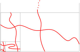 Figure 1
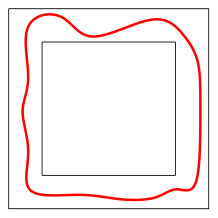 Figure 2
 Figure 3
 Figure 4
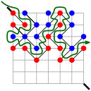 Figure 5
 Figure 6
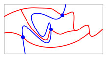 Figure 7
 Figure 8
 Figure 9
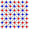 Figure 10
 Figure 11
Peer Reviews
No public reviews on file for this paper yet. If you reviewed it on a platform where reviews are public (OpenReview, ICLR, NeurIPS, ICML), you can paste yours below so the community can read it here.
Videos
No videos yet. Explain this paper in a talk, walkthrough, or lecture? Add one.
Taxonomy
TopicsAdvanced Combinatorial Mathematics · Limits and Structures in Graph Theory · Markov Chains and Monte Carlo Methods
Site Percolation on a Disordered
Triangulation of the Square Lattice
Leonardo T. Rolla
Abstract
In this paper we consider independent site percolation in a triangulation of given by adding -long diagonals to the usual graph . We conjecture that for any such graph, and prove it for almost every such graph.
1 The model
Let denote the set of squares in having all its corners in , and define the diagonal configuration space by
[TABLE]
Let denote the color configuration space
[TABLE]
Examples of a diagonal configuration and a color configuration are
[TABLE]
Let denote the probability measure on given by
[TABLE]
independently over , and let denote the law of the percolation process on the graph obtained by adding the diagonals in to the usual graph . In general, the resulting graph does not have any symmetry, but still there is a critical parameter at which the probability of having an infinite red cluster jumps from [math] to (this is a tail event).
Since this graph is a triangulation, site percolation is self-dual, that is, the only way to prevent a given red connection is with a transversal blue connection and vice-versa. This is illustrated by
[TABLE]
where existence of a left-right red crossing prevents a top-bottom blue crossing, and a left-right blue crossing prevents a top-bottom red crossing.
2 Results
Because of self-duality, the obvious conjecture111If were smaller, there would be both an infinite blue and an infinite red cluster for any , and if were larger, there would be both infinitely many red and blue circuits surrounding the origin for any . is that . In this paper we show that this is true if the diagonal configuration is obtained by tossing a fair coin for each square .
Let denote the probability on given by
[TABLE]
independently over different squares . Our sample space will be , so the process described above is governed by the “quenched measure”
[TABLE]
In this paper we will consider the “annealed measure” given by
[TABLE]
Theorem 1**.**
For the annealed process,
[TABLE]
In particular, by Fubini-Tonelli,
The proof is elementary and self-contained. The main step is to establish the analogous of Harris-FKG inequality for the annealed measure.
We note that not all events which we would normally call “increasing” are positively correlated, because two such events may have conflicting requirements for the diagonals. To overcome this, we define robust increasing events, and prove positive correlations for this type of event only.
We then show with pictures how Smirnov’s proof of RSW estimates [3, 4] and Kesten’s proof of logarithmic expected number of pivotal sites [2] can both be adapted to the present model. For completeness, we give the proof of Theorem 1 using Russo’s formula.
3 Robust increasing events
An observable is a measurable function .
Definition**.**
We say that an observable is increasing in if, for each pair , switching the color of any site from
to
increases (i.e., does not decrease) the value of .
In order to discuss monotonicity with respect to the diagonal configuration , we take into account the color configuration to see whether it is
or
who favors the
’s more than the
’s, or the other way around.
Given a color configuration , each square will be classified as having one of three types, depending on the colors of its four corners.
The first type consists of configurations whose symmetries make it impossible to decide whether
’s and
’s would prefer
or
.
– type N: \vbox{\hbox{\includegraphics[page=4,height=18.80006pt]{figures/types}}},\ \vbox{\hbox{\includegraphics[page=13,height=18.80006pt]{figures/types}}},\ \vbox{\hbox{\includegraphics[page=7,height=18.80006pt]{figures/types}}},\ \vbox{\hbox{\includegraphics[page=10,height=18.80006pt]{figures/types}}},\ \vbox{\hbox{\includegraphics[page=1,height=18.80006pt]{figures/types}}},\ \vbox{\hbox{\includegraphics[page=16,height=18.80006pt]{figures/types}}}.
Definition**.**
We say that is robust if flipping the diagonal at any square of type N does not change the value of .
Squares that are not of type N will have type A or B depending on whether it is the
’s or
’s who prefer
over
.
– type A: \vbox{\hbox{\includegraphics[page=11,height=18.80006pt]{figures/types}}},\ \vbox{\hbox{\includegraphics[page=3,height=18.80006pt]{figures/types}}},\ \vbox{\hbox{\includegraphics[page=9,height=18.80006pt]{figures/types}}},\ \vbox{\hbox{\includegraphics[page=12,height=18.80006pt]{figures/types}}},\ \vbox{\hbox{\includegraphics[page=15,height=18.80006pt]{figures/types}}}.
– type B: \vbox{\hbox{\includegraphics[page=6,height=18.80006pt]{figures/types}}},\ \vbox{\hbox{\includegraphics[page=14,height=18.80006pt]{figures/types}}},\ \vbox{\hbox{\includegraphics[page=8,height=18.80006pt]{figures/types}}},\ \vbox{\hbox{\includegraphics[page=5,height=18.80006pt]{figures/types}}},\ \vbox{\hbox{\includegraphics[page=2,height=18.80006pt]{figures/types}}}.
Definition**.**
We say that a robust observable is increasing in if, for each pair , flipping the diagonal of any square from
to
will increase for of type A and decrease for of type B. An event is called robust, increasing in and if its indicator function is so.
We mention that some events that would normally be called “increasing” are not robust. For example, in a square (what we call contains sites), existence of a red path of length connecting the top-left and bottom-right corners is not robust. Moreover, this event is not positively-correlated with existence of a red path of length connecting the top-right and bottom-left corners: they are in fact mutually exclusive. The above events are not robust because they have requirements for diagonals even when the containing squares are of type N. In the same direction, events requiring existence of disjoint paths are not robust in general.
On the other hand, and that is enough for our needs, for any sets and any domain consisting of a collection of closed squares of , the event “ is connected to by a red path in ” is both robust and increasing.
Lemma 1** (Harris-FKG).**
Let and be robust non-negative observables, increasing in and . Then
[TABLE]
Proof.
Let be fixed. For an observable , consider the projection given by . Observe that, if is robust and increasing in , then depends only on for outside the set of squares of type N. Moreover, there is a natural partial order on \{\vbox{\hbox{\includegraphics[page=1,height=11.99998pt]{figures/diagonals}}},\vbox{\hbox{\includegraphics[page=2,height=11.99998pt]{figures/diagonals}}}\}^{N_{\sigma}^{c}} under which is an increasing function (\vbox{\hbox{\includegraphics[page=1,height=11.99998pt]{figures/diagonals}}}\leq\vbox{\hbox{\includegraphics[page=2,height=11.99998pt]{figures/diagonals}}} for of type A and \vbox{\hbox{\includegraphics[page=1,height=11.99998pt]{figures/diagonals}}}\geq\vbox{\hbox{\includegraphics[page=2,height=11.99998pt]{figures/diagonals}}} for of type B). Since induces a product measure on \{\vbox{\hbox{\includegraphics[page=1,height=11.99998pt]{figures/diagonals}}},\vbox{\hbox{\includegraphics[page=2,height=11.99998pt]{figures/diagonals}}}\}^{N_{\sigma}^{c}}, projections of this type satisfy the Harris-FKG inequality with respect to . Therefore, if and are non-negative, robust and increasing in and ,
[TABLE]
We have used Fubini-Tonelli theorem for the equalities. The first inequality follows from the above observation and the second inequality follows from the standard Harris-FKG inequality, since and are increasing in . ∎
4 Proof of sharp percolation threshold
Lemma 2** (Russo-Seymour-Welsh).**
In any rectangle,
[TABLE]
In the proof we consider an exploration that progressively reveals the color of some sites and the position of some diagonals. Below we show an exploration starts from the top-left corner and targets the bottom-right corner of a rectangle. When the exploration enters a triangle by crossing one of its sides, it looks at the color of the opposite corner in order to decide on where to exit the triangle. When it enters a square, it first reveals the position of the diagonal on that square first.
[TABLE]
In this procedure, the exploration will leave the rectangle through the right side before the bottom side if there is a left-right red connection, and the bottom side before the right otherwise.
Proof of Lemma 2.
We use for . By Harris-FKG we have
[TABLE]
whence by symmetry it suffices to show that
[TABLE]
We first try to “bend” the left-side boldface region by starting an exploration path in the left-side square as shown in (1). With probability we succeed bending the boldface region until the middle of the rectangle, revealing some diagonals and some blue and red sites like this:
[TABLE]
Given a partial configuration such as above, the event in (2) is equivalent to a red connection between the two boldface regions. So we need to show that the conditional probability of such red connection is at least . But such connection is certainly implied by red path connecting two smaller boldface regions contained in a smaller grayed zone given by
[TABLE]
Now notice that none of the sites and diagonals revealed so far can interfere with this event, except for some red sites lying on the boldface region. The fact that these sites are red can only help, and the conditional probability of the latter event given that they are red is bounded from below by the probability of the crossing
[TABLE]
without any conditioning. Finally, the complementary of the latter event is
[TABLE]
which by symmetry has the same probability, concluding the proof. ∎
As usual, Lemma 2 has the following immediate corollaries.
Corollary 1**.**
There is such that, in any rectangle,
[TABLE]
Corollary 2**.**
There is such that, in any pair of co-centered squares of size and ,
[TABLE]
The last piece in the proof is the following.
Lemma 3** (Kesten).**
There is such that, for any , in any rectangle, the expected number of pivotal sites satisfies
[TABLE]
Proof.
It suffices to show that
[TABLE]
We will determine occurrence of the top-bottom blue crossing using an exploration path that starts at the top-left corner and ends at either the bottom or the right side, as below.
[TABLE]
Existence of a top-bottom blue crossing is equivalent to the exploration finding the bottom side before the right side. We want to show that, if it such crossing occurs, then the conditional expectation of the number of pivotal sites given the colors and diagonals revealed in this exploration is greater than for some constant .
On the above event, there is a self-avoiding blue path that joins the top and bottom sides of the rectangle. What we do now is a little overkilling, but it avoids the hassle of considering all corner cases related to the diagonals. Let us first inflate this self-avoiding blue path to make it squared where it would otherwise use a diagonal, as below.
[TABLE]
Notice that there are two types of sites in this squared path. The first type consists of blue sites which are adjacent to a red site which is in turn connected to the left side of the rectangle by a red path. The second type consists of sites whose color has not yet been revealed, but which are adjacent to a site of the first type.
Now, in order to find pivotal sites, we consider the domain consisting of the squares that can be reached from the right side of the big rectangle without crossing the squared path, colored in light-gray below.
[TABLE]
We will “re-sample” the entire process on this domain. Of course we cannot do that, so the red sites that we find on the squared path that turn out to have been previously sampled as blue will remain blue in the end.
We first look for a connection from the right side of the big rectangle to the squared-path that stays in a strip of width using an exploration path as below.
[TABLE]
The last red site was drawn smaller to remind us that it may be a site which we already revealed to be blue. By Corollary 1, the probability of finding such a connection is greater than .
In case such path is found, we now draw disjoint -sided and -sided squares centered at the point just found, and consider the intersection of the corresponding annuli with the light-gray region in the second previous picture. There are at least such regions that do not go lower than the bottom side of the big rectangle, minus the squares explored in the previous step, as shown below.
[TABLE]
Conditioned on the above picture, by Corollary 2 each of these “tunnels” will contain a red connection with probability at least . The conditional expectation for the number of such tunnels that actually contain such connection, given that the previous connection has been found, is thus greater than . Therefore, the conditional expectation given existence of a top-bottom blue crossing is greater than .
In the example below, two such tunnels ended up providing one red site (drawn smaller), and one of them did not.
[TABLE]
We combine the configuration discovered at this stage with the one previously removed. At this point, a small red site will become a true red site if it had not been revealed in the first exploration, and will be reverted to blue in case it had. The result is highlighted by a light-gray disk below.
[TABLE]
To conclude the proof, notice that each of these highlighted sites is either a pivotal site in case it is blue, or is preceded by a pivotal site in the squared curve in case it is red. ∎
Proof of Theorem 1.
Absence of percolation at follows from Corollary 2 as usual. Define the event
[TABLE]
in a rectangle. Using Russo’s formula and Lemma 3 we get
[TABLE]
which gives
[TABLE]
and thus, on an rectangle,
[TABLE]
To conclude the proof, we arrange rectangles as
[TABLE]
and deduce the second part of the theorem using Harris-FKG inequality. ∎
5 Extensions and alternative approaches
Recent work on Bernoulli percolation in and Voronoi percolation in provided new insights for the study of sharp phase transitions [1, 5]. It would be interesting to apply those ideas to disordered triangulations of the square lattice, and obtain alternative proofs or extend the present results to a more general setting.
Acknowledgement
I would like to thank Wendelin Werner for suggesting this problem to me back in 2009, and for inspiring discussions. I also thank him for pointing out the possible connections discussed above.
The reference list from the paper itself. Each links out to its DOI / PubMed record.
- 1[1] H. Duminil-Copin and V. Tassion. A new proof of the sharpness of the phase transition for Bernoulli percolation on Z d superscript 𝑍 𝑑 {Z}^{d} . Enseign. Math. , 62(1-2):199–206, 2016.
- 2[2] H. Kesten. The critical probability of bond percolation on the square lattice equals 1 2 1 2 \frac{1}{2} . Comm. Math. Phys. , 74(1):41–59, 1980.
- 3[3] L. Russo. A note on percolation. Z. Wahrscheinlichkeitstheorie und Verw. Gebiete , 43(1):39–48, 1978.
- 4[4] P. D. Seymour and D. J. A. Welsh. Percolation probabilities on the square lattice. Ann. Discrete Math. , 3:227–245, 1978. Advances in graph theory (Cambridge Combinatorial Conf., Trinity College, Cambridge, 1977).
- 5[5] V. Tassion. Crossing probabilities for Voronoi percolation. Ann. Probab. , 44(5):3385–3398, 2016.