Rational Solutions of the Painlev\'e-II Equation Revisited
Peter D. Miller, Yue Sheng

TL;DR
This paper reviews the algebraic properties of rational solutions to the Painlevé-II equation, explores three Riemann-Hilbert representations, and discusses their connections and asymptotic analysis using the steepest descent method.
Contribution
It compares and connects three different Riemann-Hilbert representations of rational Painlevé-II solutions and reviews recent asymptotic results derived from these frameworks.
Findings
Explicit connection between Flaschka-Newell and Bertola-Bothner representations.
Descriptions of asymptotic behavior via steepest descent method.
Clarification of algebraic and analytic properties of rational solutions.
Abstract
The rational solutions of the Painlev\'e-II equation appear in several applications and are known to have many remarkable algebraic and analytic properties. They also have several different representations, useful in different ways for establishing these properties. In particular, Riemann-Hilbert representations have proven to be useful for extracting the asymptotic behavior of the rational solutions in the limit of large degree (equivalently the large-parameter limit). We review the elementary properties of the rational Painlev\'e-II functions, and then we describe three different Riemann-Hilbert representations of them that have appeared in the literature: a representation by means of the isomonodromy theory of the Flaschka-Newell Lax pair, a second representation by means of the isomonodromy theory of the Jimbo-Miwa Lax pair, and a third representation found by Bertola and Bothner…
Click any figure to enlarge with its caption.
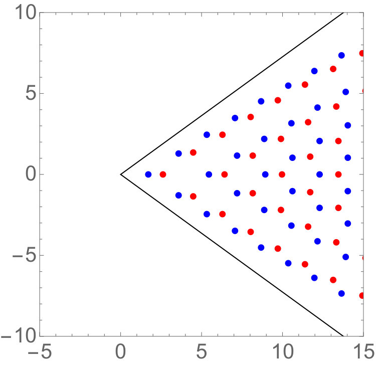 Figure 1
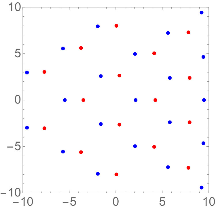 Figure 2
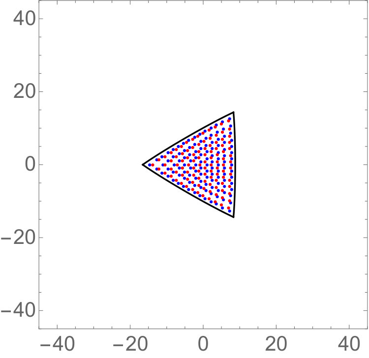 Figure 3
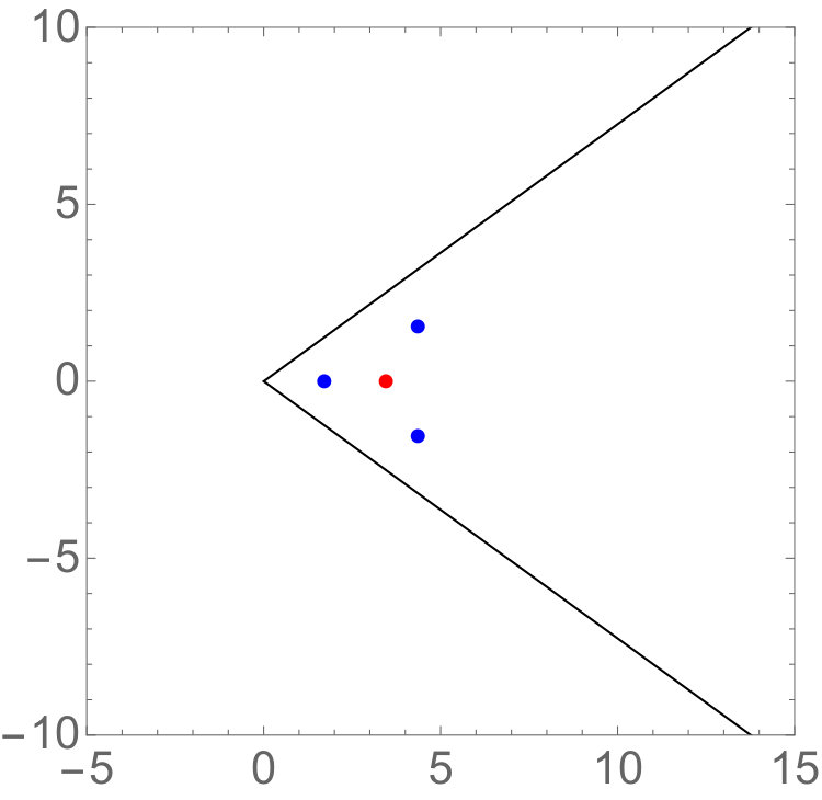 Figure 4
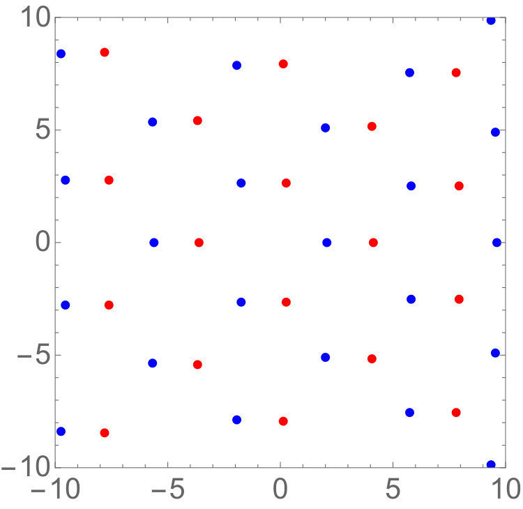 Figure 5
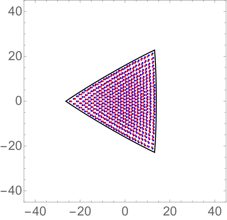 Figure 6
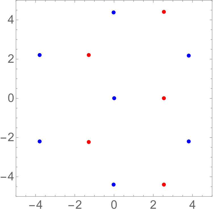 Figure 7
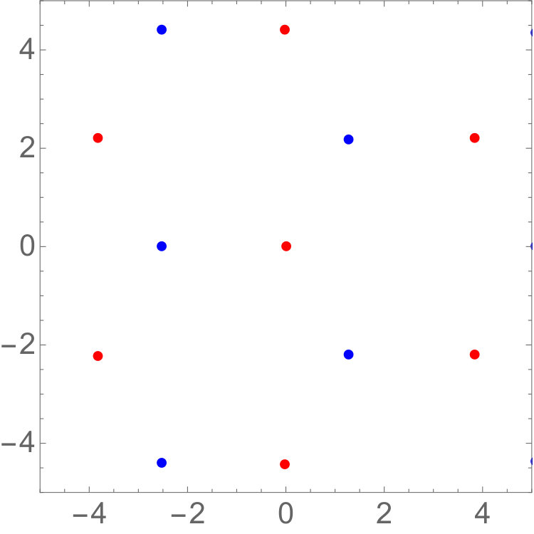 Figure 8
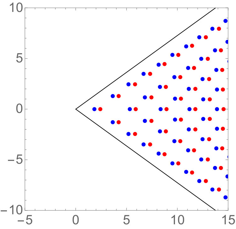 Figure 9
 Figure 10
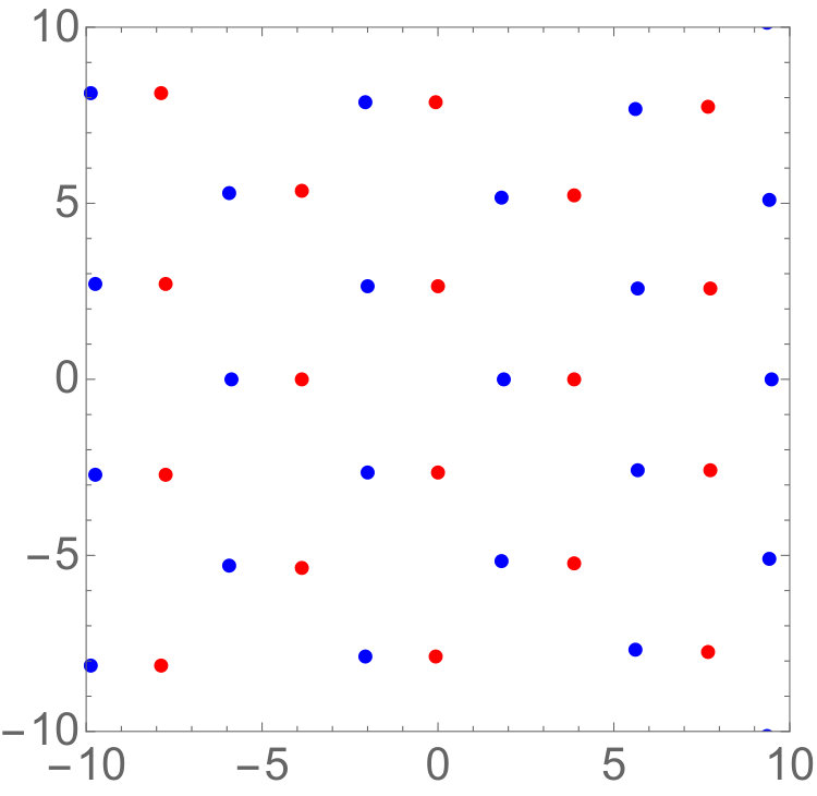 Figure 11
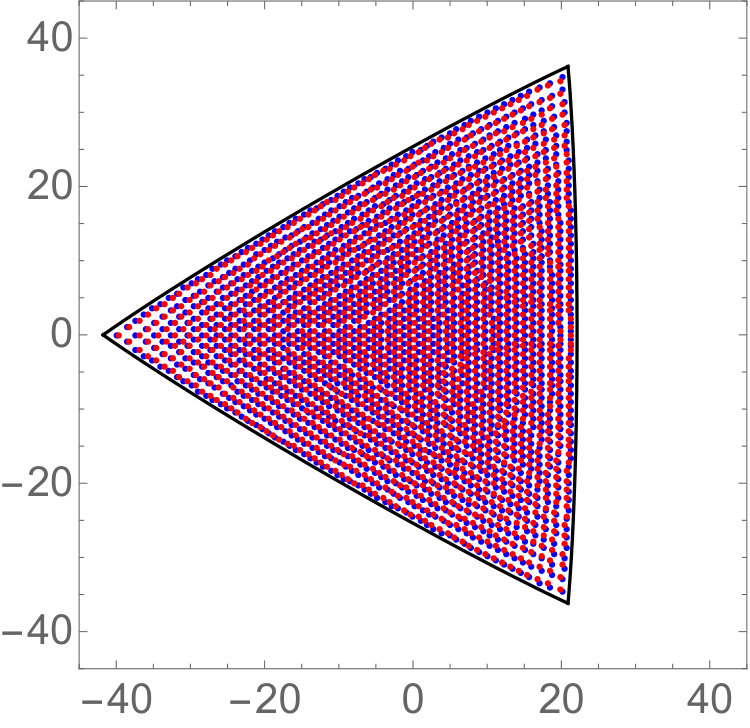 Figure 12
Peer Reviews
No public reviews on file for this paper yet. If you reviewed it on a platform where reviews are public (OpenReview, ICLR, NeurIPS, ICML), you can paste yours below so the community can read it here.
Videos
No videos yet. Explain this paper in a talk, walkthrough, or lecture? Add one.
Taxonomy
TopicsNonlinear Waves and Solitons · Advanced Differential Equations and Dynamical Systems · Quantum Mechanics and Non-Hermitian Physics
\FirstPageHeading
\ShortArticleName
Rational Solutions of the Painlevé-II Equation Revisited
\ArticleName
Rational Solutions of the Painlevé-II Equation
Revisited††This paper is a contribution to the Special Issue on Symmetries and Integrability of Difference Equations. The full collection is available at http://www.emis.de/journals/SIGMA/SIDE12.html
\Author
Peter D. MILLER and Yue SHENG \AuthorNameForHeadingP.D. Miller and Y. Sheng \AddressDepartment of Mathematics, University of Michigan,
530 Church St., Ann Arbor, MI 48109, USA \Email[email protected], [email protected] \URLaddresshttp://math.lsa.umich.edu/~millerpd/
\ArticleDates
Received April 18, 2017, in final form August 07, 2017; Published online August 16, 2017
\Abstract
The rational solutions of the Painlevé-II equation appear in several applications and are known to have many remarkable algebraic and analytic properties. They also have several different representations, useful in different ways for establishing these properties. In particular, Riemann–Hilbert representations have proven to be useful for extracting the asymptotic behavior of the rational solutions in the limit of large degree (equivalently the large-parameter limit). We review the elementary properties of the rational Painlevé-II functions, and then we describe three different Riemann–Hilbert representations of them that have appeared in the literature: a representation by means of the isomonodromy theory of the Flaschka–Newell Lax pair, a second representation by means of the isomonodromy theory of the Jimbo–Miwa Lax pair, and a third representation found by Bertola and Bothner related to pseudo-orthogonal polynomials. We prove that the Flaschka–Newell and Bertola–Bothner Riemann–Hilbert representations of the rational Painlevé-II functions are explicitly connected to each other. Finally, we review recent results describing the asymptotic behavior of the rational Painlevé-II functions obtained from these Riemann–Hilbert representations by means of the steepest descent method.
\Keywords
Painlevé equations; rational functions; Riemann–Hilbert problems; steepest descent method
\Classification
33E17; 34M55; 34M56; 35Q15; 37K15; 37K35; 37K40
1 Introduction
Rational solutions of the second Painlevé equation are important in several applied problems. It was discovered by Bass [3] that a certain Nernst–Planck model of steady electrolysis with two ions reduces to the Painlevé-II equation, and in [36] the special role of rational solutions was highlighted in the context of this model (see also [4]). Johnson [24] notes that rational solutions of the Painlevé-II equation parametrize certain string theoretic models in high-energy physics. Clarkson [11] reviews the application of rational solutions of Painlevé-II to the classification of certain equilibrium vortex configurations in ideal planar fluid flow (the poles of opposite residue determine the location of vortices of opposite circulation). More recently Buckingham and one of the authors [7] found that the collection of rational solutions of the Painlevé-II equation universally describes the space-time location of kinks in the semiclassical sine-Gordon equation near a transversal crossing of the separatrix for the simple pendulum. Also, Shapiro and Tater [37] have observed a connection between the rational Painlevé-II solutions of large degree and the characteristic polynomials for the quasi-exactly solvable part of the discrete spectrum in a boundary-value problem for the stationary Schrödinger operator with a quartic potential exhibiting PT-symmetry.
In this paper, we review some of the well-known elementary properties of the rational solutions of the Painlevé-II equation, including three ways to represent them in terms of the solution of a Riemann–Hilbert problem. We make a new contribution by showing that two of the three representations, until now thought to be unrelated, are in fact connected with each other via a simple and explicit transformation. Then we review results on the asymptotic behavior of the rational Painlevé-II solutions in the large-degree limit that have been recently obtained by analyzing these Riemann–Hilbert representations. Here our aim is to simplify the results and correct them where necessary as well as to report them in a unified context.
1.1 Basic properties of rational Painlevé-II solutions
In this paper, we consider the Painlevé-II equation with parameter written in the form
[TABLE]
1.1.1 Necessary conditions for existence of rational solutions
Obviously if , one has as a particular solution. Moreover this is the only rational solution. Indeed, any nonzero rational solution would necessarily admit, for some and , a series expansion
[TABLE]
convergent for sufficiently large , and the a dominant balance in (1.1) with would require .
Conversely, if is nonzero, (1.1) does not admit the zero solution. In this case, every rational solution again has the form (1.2) for sufficiently large and with ; it then follows from (1.1) that a dominant balance is achieved between the terms and yielding and . Therefore if is a counterclockwise-oriented circle of sufficiently large radius,
[TABLE]
Likewise if is a finite pole of order of the rational solution , then the substitution of the Laurent series
[TABLE]
into (1.1) results in a dominant balance between and yielding and , so every pole of is simple and has residue . If denotes the number of poles of of residue , then
[TABLE]
so comparing with (1.3), we see that (1.1) admits a rational solution only if .
1.1.2 Bäcklund transformations. Sufficient conditions for existence
of rational solutions. Uniqueness
In 1971, Lukashevich [31] discovered an explicit Bäcklund transformation for (1.1). Namely, supposing that is an arbitrary solution of (1.1), the related function defined111The definition apparently fails if is such that vanishes identically. It is easy to check that this condition is consistent with (1.1) only if (so the numerator in (1.4) vanishes also). In the case , the Riccati equation is solved by the formula where ; in other words, is an Airy function and is a known special function (Airy) solution of (1.1). A similar remark applies to the inverse transformation (1.5) which gives and the denominator vanishes for the Airy solutions. Note that both transformations (1.4) and (1.5) make sense whenever except possibly for isolated values of . by
[TABLE]
satisfies (1.1) with replaced by . Note that is a rational function whenever is; therefore from the “seed solution” for , the (iterated) Bäcklund transformation produces a rational solution of (1.1) for every positive integer . From the elementary symmetry of (1.1) one then has the existence of a rational solution of (1.1) for every , a fact that also follows from the earlier work of Yablonskii [39] and Vorob’ev [38] (see Section 1.1.3 below). Hence, as pointed out by Airault [1], the condition is both necessary and sufficient for the existence of rational solutions to (1.1).
The Bäcklund transformation (1.4) also yields a proof of uniqueness of the rational solution for given , a fact that was first noted by Murata [32]. Indeed, combining (1.4) with the symmetry yields a second Bäcklund transformation
[TABLE]
taking solving (1.1) to solving (1.1) with replaced by . Importantly, an elementary computation shows that the Bäcklund transformations (1.4) and (1.5) are inverses of each other on the space of solutions of (1.1). In particular, both are injective maps. Suppose and are distinct rational solutions of (1.1) for some . Iteratively applying either (1.4) (if ) or (1.5) (if ) times, by injectivity we arrive at two distinct rational solutions of (1.1) with in contradiction with the already-established uniqueness of the rational solution for . See [17] for further information about Bäcklund transformations for Painlevé equations.
Explicitly, the first several rational Painlevé-II solutions are
[TABLE]
where the subscript indicates the value of in (1.1).
1.1.3 Representation in terms of special polynomials
It was first observed by Yablonskii [39] and Vorob’ev [38] that rational solutions of the Painlevé-II equation (1.1) can be represented in terms of special polynomials having an explicit recurrence relation. The Yablonskii–Vorob’ev polynomials are defined recursively by , , and then
[TABLE]
Then the rational solution of (1.1) can be expressed as
[TABLE]
Of course the first surprise regarding the recursion formula (1.7) is that is indeed a sequence of polynomials in . Indeed this is the case, as can be seen by the alternative formula due to Kajiwara and Ohta [26] expressing as a constant multiple of the Wronskian of polynomials in (see also [10, Section 2.4]), and the first several iterates of (1.7) produce:
[TABLE]
It has been shown that the polynomials all have simple roots and that and can have no roots in common [20], facts that are consistent via (1.8) with the fact that all poles of are simple with residues . Real roots of the Yablonskii–Vorob’ev polynomials correspond to real poles of , and these have been studied extensively by Roffelsen who has shown that all nonzero real roots are all irrational [34] and that there are precisely negative roots of and total real roots of , and if and only if [35]. Also, the real roots of and interlace, as was proven by Clarkson [10].
1.2 Outline of the paper
The fact that all rational solutions of the Painlevé-II equation (1.1) can be iteratively constructed, either via the direct Bäcklund transformations (1.4) and (1.5) or via the recurrence relation for the Yablonskii–Vorob’ev polynomials (1.7), is quite remarkable and indicative of deeper integrable structure underlying the Painlevé-II equation. However, it must also be pointed out that the use of these iterative constructions is limited in practice, because the formulae generated become increasingly complicated as increases. The situation is similar to that encountered when studying orthogonal polynomials, which in general can be constructed systematically by a Gram–Schmidt orthogonalization algorithm, but the number of steps of this algorithm increases with the degree of the polynomial desired, making it difficult to appeal to this approach to deduce properties of the general polynomial in the family.
Therefore, if our interest is to understand the analytic properties of the rational Painlevé-II functions, it is necessary to have an alternative representation that admits the possibility of asymptotic analysis for large . In Section 2 we describe three such representations of the rational Painlevé-II solutions, two coming directly from the isomonodromic integrable structure underlying the Painlevé-II equation, and one related to a recently discovered representation of the squares of the Yablonskii–Vorob’ev polynomials in terms of the integrable structure behind orthogonal polynomials (which provides a work-around for the Gram–Schmidt procedure allowing large-degree asymptotics of general orthogonal polynomials to be computed). One of the contributions of our paper is then to establish a new identity relating the orthogonal polynomial approach to one of the isomonodromic approaches; see Section 2.4.
These representations of the rational Painlevé-II solutions have indeed proven to be useful in characterizing the rational functions in the limit of large . In Section 3 we review some of the results that have been proven with their help, outlining some of the methods of proof.
Below we will make frequent use of the Pauli spin matrices defined by
[TABLE]
2 Riemann–Hilbert problem representations
of the rational Painlevé-II solutions
2.1 Flaschka–Newell representation
In 1980, Flaschka and Newell [16] showed how a self-similar reduction of the Lax pair representation of the modified Korteweg–de Vries equation reveals the Painlevé-II equation in the form (1.1) to be an isomonodromic deformation of the linear equation
[TABLE]
in which , , , and are regarded as numerical parameters. Indeed, (2.1) is compatible with the auxiliary linear equation
[TABLE]
only if the compatibility condition
[TABLE]
holds with and . This forces to depend on by the Painlevé-II equation in the form (1.1) and forces . The equation (2.2) then implies that the monodromy data associated with solutions of (2.1) depends trivially on .
Let us describe the monodromy data associated with rational solutions of (1.1) for . It is pointed out in [16] that whenever in (2.1) for the rational solution , the irregular singular point at for (2.1) exhibits only trivial Stokes phenomenon. This implies the existence of a fundamental solution matrix of (2.1) of the form
[TABLE]
for some matrix coefficients , , and so on, where
[TABLE]
and where the infinite series in (2.4) is convergent for sufficiently large, which in view of being the only finite singular point actually means for . Assuming compatibility, i.e., that solves (1.1) with , it can be shown that is also a fundamental solution matrix for (2.2), and then it follows by substitution into the latter system that is recovered from the subleading term of the expansion (2.4) by the formula
[TABLE]
On the other hand, is a regular singular point for (2.1). Applying the method of Frobenius, there exists a fundamental solution matrix of (2.1) defined in a neighborhood of having the form
[TABLE]
for some scalar function and matrix coefficients , , and so on. The absence of logarithms in spite of the fact that the Frobenius exponents differ by an integer follows from the fact that, due to the triviality of the Stokes phenomenon at , the monodromy matrix for (2.1) corresponding to any loop about the origin is the identity, hence diagonalizable. However the same fact implies an ambiguity in the formula (2.6) in which the dominant column in the limit is only determined up to addition of a multiple of the subdominant column. Flaschka and Newell [16] resolve this ambiguity as follows. They first observe that the subdominant column is well-defined after the choice of the scalar , and from the recurrence relations determining the higher-order terms from the preceding terms a predictable pattern emerges in which consecutive terms are alternating scalar multiples of the vectors and . A similar well-defined alternating pattern holds for the dominant column, but only through the terms with , with the term for satisfying an equation that is consistent but indeterminate. Here a choice is made: the term for is taken to continue the alternating pattern of vectors and . Once this choice has been made, the alternating pattern again continues to all orders of the dominant column. In other words, Flaschka and Newell take in the more specific form
[TABLE]
There is then exactly one matrix solution of (2.1) of this form for a given scalar , and moreover, assuming compatibility, can be chosen up to a constant scalar multiple so that simultaneously solves (2.2). Again, the infinite series appearing in (2.7) is convergent near , and since there are no other finite singular points it is actually convergent for all . By taking the limits and respectively, Abel’s theorem implies the identities and because the coefficient matrix in (2.1) has zero trace. Therefore, as both and (for a suitable choice of ) are simultaneous fundamental solution matrices for (2.1) and (2.2) defined in a common domain , there exists a constant unimodular matrix such that
[TABLE]
The connection matrix is the monodromy data for the linear problem (2.1) in the case that is a rational solution of (1.1). For more general solutions given , or for non-integral values of , the monodromy data becomes augmented with six Stokes matrices of alternating triangularity connecting solutions each having the form (2.4) (but only as an asymptotic series, with no convergence properties implied) in six overlapping sectors of the irregular singular point at .
It is easy to see that is a fundamental solution matrix for the system (2.1) whenever is. This substitution also leaves (2.2) invariant. Since is uniquely determined from (2.1) and the leading term of its large- asymptotic expansion (convergent in the trivial-monodromy case at hand for rational solutions ), we deduce the identity
[TABLE]
Similarly, given the scalar , it follows from (2.7) that
[TABLE]
Therefore, conjugating by and replacing in (2.8), the use of the identities (2.9)–(2.10) shows that also
[TABLE]
and hence comparing again with (2.8) one sees that . This matrix identity along with the condition that implies that necessarily has the form
[TABLE]
where only the nonzero constant is undetermined by symmetry.
We may now formulate a Riemann–Hilbert problem to recover and , and hence also the rational Painlevé-II function , from the monodromy data, i.e., from the connection matrix . To this end, we define a matrix by
[TABLE]
It is then clear that solves the following Riemann–Hilbert problem.
Riemann–Hilbert Problem 2.1** (Flaschka–Newell representation).**
Let and be given. Seek a matrix-valued function defined for , , with the following properties:
- •
Analyticity.* is analytic for , taking continuous boundary values and for from the interior and exterior respectively of the unit circle.*
- •
Jump condition.* The boundary values are related by*
[TABLE]
- •
Normalization.* The matrix is normalized at as follows:*
[TABLE]
where the limit may be taken in any direction.
The solution of this Riemann–Hilbert problem exists precisely for those values of that are not poles of . Given the solution , one extracts the rational Painlevé-II function from the limit (cf. (2.5))
[TABLE]
Note also that without loss of generality one may take the constant in (2.11) to be , simply by re-defining within the unit circle by multiplication on the right by . Such a re-definition clearly does not affect for and therefore has no essential effect on the reconstruction of .
Flaschka and Newell observe that Riemann–Hilbert Problem 2.1 can be solved by reduction to finite-dimensional linear algebra, resulting in determinantal formulae for equivalent to iterated Bäcklund transformations studied by Airault [1]. To see this, note that uniqueness of solutions of Riemann–Hilbert Problem 2.1 is an elementary consequence of Liouville’s theorem, so it is sufficient to construct a solution by any means. Now, necessarily has a convergent Laurent expansion about , suggesting to seek as a suitable Laurent polynomial. In fact, assuming without loss of generality that , we may suppose that in the domain the first row of has the form
[TABLE]
This ansatz clearly satisfies the necessary analyticity condition for as well as the normalization condition at . The jump condition can then be reinterpreted as requiring that the linear combinations
[TABLE]
where the boundary values and are given by the ansatz (2.13), both be analytic functions within the unit disk, where the only potential singularity is . The form of the ansatz automatically guarantees that this is the case for , but has precisely negative powers of whose coefficients are required to vanish. It is easily seen that this amounts to a square inhomogeneous linear system of equations, explicit in terms of the Taylor coefficients of , on the unknowns and . The solution of this linear system by Cramer’s rule gives the rational Painlevé-II function in the form . For example, in the case we require that
[TABLE]
where the last term represents a function analytic at , be analytic at from which one obtains as expected (cf. (1.6)).
2.2 Jimbo–Miwa representation
In 1981, Jimbo and Miwa [23] found a representation of the Painlevé-II equation as the compatibility condition for a Lax pair different from that found by Flaschka and Newell. We take Jimbo and Miwa’s linear equations in the form
[TABLE]
and
[TABLE]
For this system, the compatibility condition (2.3) with and is equivalent to the following first-order system of equations:
[TABLE]
This system admits a first integral
[TABLE]
and then with the system (2.16) yields the Painlevé-II equation for in the form (1.1).
As with the Flaschka–Newell approach, it is the problem (2.14) whose analysis for fixed determines the monodromy data, which is then independent of for simultaneous solutions of (2.14)–(2.15). However, the direct monodromy problem (2.14) has a different character than in the Flaschka–Newell approach because (2.14) has only one singular point, an irregular singular point at infinity, while (2.1) has in addition a regular singular point at the origin if . Thus, all solutions of (2.14) are entire functions of , and all monodromy data is generated only from the Stokes phenemonon about the singular point at infinity. In particular, it is the case that for the rational solution for , solutions of (2.14) exhibit nontrivial Stokes phenomenon in contrast to the situation in Flaschka–Newell theory.
The Stokes multipliers for (2.14) when is the rational solution of (1.1) for can be inferred from the following Riemann–Hilbert problem, which arises naturally in the study of solutions of the sine-Gordon equation in the semiclassical limit near certain critical points ; see [7, Section 5].
Riemann–Hilbert Problem 2.2** (Jimbo–Miwa representation).**
Let and be given. Seek a matrix-valued function be defined for , where is the union of six rays , and having the following properties:
- •
Analyticity.* is analytic for , taking continuous boundary values along the boundary of each component of this domain.*
- •
Jump condition.* Taking each ray of to be oriented in the direction away from the origin and given a point on one of the rays using the notation *resp. to denote the boundary value taken at from the left resp. right, the boundary values are related by
[TABLE]
where is constant along each ray and is as shown in Fig. 1.
- •
Normalization.* The matrix is normalized at as follows:*
[TABLE]
where the limit can be taken in any direction except the positive real axis, which is the branch cut for the principal branch of .
From the solution of Riemann–Hilbert Problem 2.2 one obtains the rational Painlevé-II function from the coefficients in the large- expansion of :
[TABLE]
by the formula
[TABLE]
In [7], it was deduced that Riemann–Hilbert Problem 2.2 encodes the Stokes multipliers for the Lax pair (2.14)–(2.15) associated with the rational Painlevé-II function as follows. Firstly, by considering , one shows that partial derivatives of with respect to and satisfy exactly the same jump conditions on the rays of as does itself, a fact that along with some local analysis near and shows that is a simultaneous fundamental solution matrix of the two Lax pair equations (2.14)–(2.15), provided that the coefficients , , , and are defined from the expansion (2.18) by the formulae
[TABLE]
Then, by reexamination of the asymptotic behavior of for large one finds that the parameter appearing in Riemann–Hilbert Problem 2.2 is related to these functions by the identity (2.17), identifying it with the parameter appearing in the Painlevé-II equation (1.1). It remains therefore to deduce that defined now by the expression (2.19) is the rational solution of (1.1). This can be accomplished by first noting that in the case a symmetry argument combined with (2.19) shows that , at which point one can leverage the -part (2.15) of the Lax pair to construct explicitly in terms of Airy functions of argument 6^{-1/3}\big{(}y+\tfrac{3}{2}\zeta^{2}\big{)}. Then, one can apply iterated discrete isomondromic Schlesinger transformations (also known in the integrable systems literature as Darboux transformations; see [6, Section 2] and [23] for further information on these notions) to explicitly increment or decrement the value of in integer steps, with the corresponding effect on the coefficient defined by (2.19) being given by the Bäcklund transformations (1.4) or (1.5) respectively. As these preserve rationality, one concludes that given by (2.19) is precisely the rational solution of (1.1) when is the solution of Riemann–Hilbert Problem 2.2 for arbitrary . See [7, Section 5] for full details of these arguments.
2.3 Bertola–Bothner representation
In [5], Bertola and Bothner derived a new Hankel determinant representation of the squares of the Yablonskii–Vorob’ev polynomials defined by the recurrence relation (1.7) with initial conditions and . This new identity leads to a formula expressing the rational Painlevé-II function in terms of pseudo-orthogonal polynomials (i.e., polynomials orthogonal with respect to an indefinite inner product involving contour integration with a complex-valued weight), and this in turn leads to a Riemann–Hilbert representation.
The main theorem reported and proved in [5] is the following.
Theorem 2.3** (Bertola and Bothner, [5]).**
Given , let denote the Taylor coefficients of the generating function :
[TABLE]
Then, for any ,
[TABLE]
where denotes the greatest integer less than or equal to and is the Hankel determinant
[TABLE]
The coefficients are polynomials with numerous special properties, some of which are enumerated in [5]. Similar determinantal representations of the Yablonskii–Vorob’ev polynomials themselves (not the squares) had been previously known [26], including one representing via a non-Hankel determinant involving the scaled functions \mu_{k}\big{(}4^{1/3}z\big{)} and one representing as a Hankel determinant built from functions that can be extracted from a generating function via a non-convergent asymptotic series [21]. However, it is the combination of the Hankel structure of the determinant with the convergent nature of the generating function expansion that leads to a Riemann–Hilbert representation of as we will now explain.
When combined with Theorem 2.3, the representation (1.8) of in terms of the Yablonskii–Vorob’ev polynomials gives
[TABLE]
Now, since the polynomials are Taylor coefficients of the entire function , they may be written as contour integrals using the Cauchy integral formula:
[TABLE]
Here is a simple contour encircling the origin in the counterclockwise direction; without loss of generality we will take it to coincide with the unit circle. Setting in the integrand puts the formula in the equivalent form
[TABLE]
where may be taken to be the same contour, and where
[TABLE]
Thus, are revealed as the monomial moments of a complex-valued weight parametrized by and defined on the unit circle. This fact immediately gives an interpretation to the ratio of consecutive Hankel determinants (cf. (2.20)); it is the norming constant of the monic pseudo-orthogonal polynomial defined given by the pseudo-orthogonality conditions
[TABLE]
Indeed, if exists222Existence is not guaranteed for every because integration against does not define a definite inner product, nor does (2.21) represent Hermitian orthogonality which would require replacing with its complex conjugate. Hence the terminology of “pseudo-orthogonality”. for the given value of then it follows that
[TABLE]
The points where either \psi_{m}\big{(}\xi;\big{(}\tfrac{2}{3}\big{)}^{1/3}y\big{)} fails to exist or \eta_{m}\big{(}\big{(}\tfrac{2}{3}\big{)}^{1/3}y\big{)}=0 (but possibly not both, should cancellation occur) are precisely the poles of .
Now, it is well-known that given any complex measure on a suitable contour, the corresponding pseudo-orthogonal polynomial of degree can be characterized via the solution of a matrix Riemann–Hilbert problem of Fokas–Its–Kitaev type [18]. In the present context, that Riemann–Hilbert problem is the following.
Riemann–Hilbert Problem 2.4** (Bertola–Bothner representation).**
Let be an integer, and let be given. Seek a matrix-valued function defined for , , with the following properties:
- •
Analyticity.* is analytic for , taking continuous boundary values and for from the interior and exterior respectively of the unit circle.*
- •
Jump condition.* The boundary values are related by*
[TABLE]
- •
Normalization.* The matrix is normalized at as follows:*
[TABLE]
where the limit may be taken in any direction.
Indeed, all of the relevant quantities associated with the pseudo-orthogonal polynomials for the weight are encoded in the solution of this problem. In particular,
[TABLE]
from which it follows (cf. (2.21)–(2.22)) that
[TABLE]
Asymptotic analysis of the pseudo-orthogonal polynomials in the limit of large can therefore be carried out by applying steepest descent techniques to Riemann–Hilbert Problem 2.4, as was first done in the case of true orthogonality on the real line in [14] and in the case of true orthogonality on the unit circle in [2]. However, noting that the expression (2.20) involves differentiation with respect to the parameter , a limit process that cannot be assumed to commute with the limit , Bertola and Bothner show how to obtain the relevant derivatives directly from the solution of Riemann–Hilbert Problem 2.4. The essence of the argument is as follows. The related matrix must be analytic for and satisfies jump condition across the unit circle of exactly the form (2.23) in which has been replaced by . As the parameter no longer appears in the jump matrix for , it follows that the partial derivative also satisfies exactly the same jump condition, and therefore the matrix ratio has no jump and so extends to an analytic function on the punctured complex plane . The asymptotic behavior of for large and small is easily expressed in terms of :
[TABLE]
where as . Therefore is a -dependent multiple of given by two equivalent formulae:
[TABLE]
From the -entry in this matrix identity one obtains
[TABLE]
where we have used the fact that the necessarily unique solution of Riemann–Hilbert Problem 2.4 has unit determinant. Therefore, from the solution of Riemann–Hilbert Problem 2.4 the rational Painlevé-II function can be expressed without differentiation with respect to as
[TABLE]
for .
2.4 Explicit relation between the Flaschka–Newell
and Bertola–Bothner representations
The Riemann–Hilbert representations of the rational Painlevé-II functions appearing in the isomonodromy approaches of Flaschka–Newell (cf. Section 2.1) and Jimbo–Miwa (cf. Section 2.2) are known to be related. Indeed, Joshi, Kitaev, and Treharne found an explicit integral transform relating simultaneous solutions of the corresponding Lax pairs [25, Corollary 3.2]. This integral transform provides another explanation for the fact that the solution of Riemann–Hilbert Problem 2.1 is rational in while that of Riemann–Hilbert Problem 2.2 is transcendental in , being built from Airy functions [7]. The approach of Bertola–Bothner also leads to a Riemann–Hilbert representation of the rational Painlevé-II functions, but the approach is not motivated by isomonodromy theory for any Lax pair, so it seems more mysterious from this point of view. In this section we show that the Riemann–Hilbert problem appearing in the Bertola–Bothner approach is in fact explicitly connected to that arising in the Flaschka–Newell isomonodromy theory:
Theorem 2.5**.**
Let be an integer, suppose that is not a pole of the rational Painlevé-II function , and let z=\big{(}\tfrac{2}{3}\big{)}^{1/3}y. Then the unique solution of Riemann–Hilbert Problem 2.1 arising from Flaschka–Newell theory is related to the unique solution of Riemann–Hilbert Problem 2.4 arising from the Bertola–Bothner approach by an explicit elementary transformation with an explicit elementary inverse cf. equations (2.25)–(2.27), (2.29), (2.30), (2.34), and (2.36) in the proof below.
Proof.
We start with the Flaschka–Newell approach and Riemann–Hilbert Problem 2.1. Suppose without loss of generality that . We begin by noting that the matrix defined by (2.11) has the lower-upper factorization
[TABLE]
and therefore the jump matrix in Riemann–Hilbert Problem 2.1 is
[TABLE]
and the right-hand factor is obviously analytic within the unit disk and has unit determinant. Therefore, defining a new matrix in terms of the unknown by
[TABLE]
we see that satisfies exactly the same conditions as specified in Riemann–Hilbert Problem 2.1 except that the jump condition across the unit circle becomes instead
[TABLE]
This triangular jump matrix already suggests the Fokas–Its–Kitaev form that appears in the approach of Bertola and Bothner, but we require two more steps to complete the identification. Firstly, we make the simple substitution
[TABLE]
where
[TABLE]
Now observe that the following Riemann–Hilbert problem captures at the same time the matrix and the matrix appearing in the Bertola–Bothner approach, for different values of the auxiliary parameter .
Riemann–Hilbert Problem 2.6**.**
Let , , and be given. Seek a matrix-valued function defined for , , with the following properties:
- •
Analyticity.* is analytic for , taking continuous boundary values** and for from the interior and exterior respectively of the unit circle.*
- •
Jump condition.* The boundary values are related by*
[TABLE]
- •
Normalization.* The matrix is normalized at as follows:*
[TABLE]
where the limit may be taken in any direction.
Indeed, it is easy to check that
[TABLE]
by comparison with the conditions of Riemann–Hilbert Problems 2.1 and 2.4. We complete the connection between the Flaschka–Newell and Bertola–Bothner approaches by next establishing the relation between solutions for consecutive values of .
The solution of Riemann–Hilbert Problem 2.6 has a convergent Laurent expansion for large of the form
[TABLE]
for some residue matrix . Noting that if it exists for a given , the unique solution of Riemann–Hilbert Problem 2.6 has unit determinant, consider the matrix defined by
[TABLE]
It is straightforward to check from (2.28) that the boundary values taken by on the unit circle satisfy the trivial jump condition for ; hence extends to the whole complex plane as an entire function of . Moreover, using (2.30) it follows that has the following asymptotic expansion for large :
[TABLE]
It then follows by Liouville’s theorem that all negative power terms in the Laurent expansion of vanish, i.e., is the linear function of given by the explicit matrix on the second line of (2.32). Returning to (2.31), we have established the identity
[TABLE]
If we can express the second column of in terms of , then this becomes an explicit formula for in terms of the latter.
To this end, consider the second column of (2.33) evaluated at , which reads
[TABLE]
because and are analytic at . Therefore,
[TABLE]
so substituting into (2.33) we recover the explicit formula for decrementing the value of :
[TABLE]
In a similar way, the matrix
[TABLE]
is an entire function that equals the polynomial part of its Laurent expansion for large , and hence
[TABLE]
leading to the following analogue of (2.33):
[TABLE]
From the first column of (2.35) evaluated at we get
[TABLE]
so substituting into (2.35) we recover the explicit formula for incrementing the value of :
[TABLE]
Note that equations (2.34) and (2.36) can be interpreted as discrete Schlesinger/Darboux transformations (see [6, Section 2] and [23]) for Riemann–Hilbert Problem 2.6.
Taking into account the explicit and obviously invertible transformations (2.25)–(2.27) relating solving Riemann–Hilbert Problem 2.1 to via , the formulae (2.34) and (2.36) establish the connection with Riemann–Hilbert Problem 2.4 having solution . ∎
We remark that although Theorem 2.5 provides an explicit relation between the solutions of Riemann–Hilbert Problems 2.1 and 2.4, it can happen that for given one of these problems is solvable and the other is not. This occurs precisely when one of the denominators in (2.34) or in (2.36) vanishes. Indeed, we have mentioned before (and it actually follows from the formula (2.12)) that the points where Riemann–Hilbert Problem 2.1 fails to be solvable correspond precisely to the poles of . On the other hand, the formula (2.24) shows that it is possible that some poles of can arise from the well-defined function vanishing at a point where Riemann–Hilbert Problem 2.4 has a solution; hence Riemann–Hilbert Problem 2.4 is solvable while Riemann–Hilbert Problem 2.1 is not. It can also happen that Riemann–Hilbert Problem 2.4 fails to be solvable at a point corresponding to a regular point of and hence a point of solvability of Riemann–Hilbert Problem 2.1, in which case the formula (2.24) retains sense locally via a limit process (i.e., l’Hôpital’s rule).
3 Asymptotic behavior of the rational Painlevé-II functions
3.1 Numerical observations and heuristic analysis
In this section, we assume without loss of generality that . There have been several studies of the rational solutions of the Painlevé-II equation from the numerical point of view, mostly concerned with looking for patterns in the distribution of poles of in the complex -plane as varies. The earliest work in this direction that we are aware of is the 1986 paper of Kametaka et al. [27] in which numerical methods were brought to bear on the problem of finding roots of the Yablonskii–Vorob’ev polynomials for as large as ; the figures in [27] for the largest values of display features suggesting the breakdown of the numerical method. A figure such as those from [27] also appears in the 1991 monograph [22]. These studies show the poles of being contained for reasonably large within a roughly triangular-shaped region of size increasing with and therein organized in an apparently regular, crystalline pattern. Plots of poles of obtained by similar methods also appear in [12], a paper that includes in addition a study of corresponding phenomena in higher-order equations in the Painlevé-II hierarchy. More recently, general numerical methods for the study of solutions with many poles in differential equations have been advanced based on such techniques as Padé approximation, and these methods have been shown to be capable of accurately reproducing the pole pattern of , treating the Painlevé-II equation (1.1) as an initial-value problem to be solved numerically taking as initial conditions the exact values of and [19, 33]. In Fig. 2 we give our own plots of poles of for , , and , which we made by symbolically constructing the relevant Yablonskii–Vorob’ev polynomials in Mathematica and using NSolve with the option WorkingPrecision->50 to find the roots.
These numerical observations suggest structure that should be explained, and yet the large- limit in which the structural features of interest appear to become clear in the numerics is fundamentally out of reach of exact methods like iterated Bäcklund transformations or explicit determinantal formulae, the study of which becomes combinatorially prohibitive in this limit. Therefore one may consider instead methods of asymptotic analysis. A formal approach may be based upon the observation that the modulus of the poles or zeros of most distant from the origin scales roughly like [22], which suggests examining in a small neighborhood of a point ; dominant balance arguments suggest that the size of the neighborhood should then be proportional to . So, letting be fixed, consider the change of independent variable in (1.1) given by (the relatively small shifts by are convenient for later but at this point are inconsequential)
[TABLE]
Substituting this into (1.1) along with the scaling of the independent variable by p=\big{(}m-\tfrac{1}{2}\big{)}^{1/3}\mathcal{P}, one arrives at the equivalent equation
[TABLE]
which for large appears to be a perturbation of an autonomous equation for an approximating function :
[TABLE]
Multiplying by and integrating gives
[TABLE]
where is an integration constant. If and are related in such a way that the quartic polynomial on the right-hand side of (3.2) has a double root , then is an equilibrium solution of (3.1). Double roots are necessarily related to via the cubic equation
[TABLE]
and then the relation between and guaranteeing the existence of the double root can be expressed in terms of a solution of (3.3) by
[TABLE]
It turns out (see Section 3.3.1 below) that this approximation of by the equilibrium solution accurately describes the rational Painlevé-II function in the pole-free region, provided that one selects the (unique) solution of (3.3) with the asymptotic behavior {\widetilde{\mathcal{P}}}_{0}(x)=x^{-1}+\mathcal{O}\big{(}x^{-2}\big{)} as . This solution has branch points at and for , which correspond to the corners of the triangular-shaped region containing the poles. More general solutions of (3.1) can be expressed as elliptic functions of with elliptic modulus depending on the parameters and . These also turn out to be important in describing the rational Painlevé-II functions in the interior of the triangular region. Indeed, if one fixes a value of sufficiently small to correspond to in the triangular region and views the rational Painlevé-II functions as functions of the variable , one sees increasingly regular patterns of poles in the limit suggestive of the period parallelogram of an elliptic function of . See Fig. 3.
A similar formal scaling argument can be applied to study the asymptotic behavior of near the corner points of the triangular region. For example, to zoom in on the corner point on the negative real axis, we may make the scalings
[TABLE]
after which one sees that the Painlevé-II equation (1.1) takes the form
[TABLE]
for and bounded, i.e., a perturbation of the Painlevé-I equation. This is a well-known degeneration of the Painlevé-II equation [28, 30], and it suggests that particular solutions of the Painlevé-I equation may play a role in the asymptotic description of near the three corner points. This also turns out to be true (see Section 3.3.4).
3.2 The elliptic region and its boundary
Let denote the solution of the cubic equation (3.3) with {\widetilde{\mathcal{P}}}_{0}(x)=x^{-1}+\mathcal{O}\big{(}x^{-2}\big{)} as , which can be analytically continued to a maximal domain consisting of the complex -plane omitting three line segments connecting the three points , with the origin. For , let denote the function defined to satisfy and as , defined on a maximal domain of analyticity in the -plane333The complex variable (written as in [8, 9]) is a rescaling of the variable from Riemann–Hilbert Problem 2.2. omitting only the segment connecting the roots of , one of which we denote by . We define a function by
[TABLE]
where the path of integration is arbitrary444It can be checked that the value of is unchanged by adding loops around the branch cut of to the path of integration because satisfies (3.3). within the domain of analyticity of .
It turns out that in the limit , the region of the complex plane that contains the poles of is , where is the bounded component of the set of for which . The boundary consists of points for which . The integral in (3.5) can be evaluated in terms of elementary functions, taking appropriate care of branches of multivalued functions; expressions can be found in [5, 8]. The exact formula is less important than the basic property that is analytic for with algebraic branch points at the points and . This implies that is a union of three analytic arcs joining the branch points pairwise, with reflection symmetry in the real axis and rotation symmetry about the origin by integer multiples of . The curve is superimposed on each of the pole plots in Fig. 2. We call the elliptic region, the three branch points of its corners, and the three smooth arcs of its edges. Local analysis of shows [9, Section 2.3] that the interior angles of at the three corners are all , so that is a “curvilinear triangle” at best.
3.3 Asymptotic description of by steepest descent
We now present several results on the asymptotic behavior of the rational Painlevé-II function , all of which have been obtained by the application of variants of the Deift–Zhou steepest descent method [15] to either Riemann–Hilbert Problem 2.2 (see [8, 9]) or Riemann–Hilbert Problem 2.4 (see [5]). Regardless of which Riemann–Hilbert problem is the starting point, the basic steps of the method are the same:
Introduce a diagonal matrix multiplier built from exponentials of a scalar function frequently called a “-function” with the aim of simultaneously obtaining normalization to the identity matrix at infinity and stabilizing the jump matrices of the problem so that they are alternately exponentially small perturbations of either constant matrices or purely oscillatory matrices along different contour arcs. Frequently this step also requires some deformation of the contour of the original Riemann–Hilbert problem by means of analytic continuation of the jump matrices. 2. 2.
Use explicit matrix factorizations to algebraically separate oscillatory factors in the jump matrices having phase derivatives of opposite signs. Splitting the jump contour into separate arcs for each factor, a subsequent deformation to either side of the original jump contour ensures that the oscillatory factors now become exponentially small in the limit . 3. 3.
Construct an explicit model of the solution called a “parametrix” by considering only those remaining jump matrices that are not exponentially small perturbations of the identity matrix. 4. 4.
By comparing the unknown matrix obtained after the second step with the parametrix, obtain an equivalent Riemann–Hilbert problem for the matrix quotient. The aim of the method is to ensure that the resulting Riemann–Hilbert problem is of “small-norm” type, meaning that it can be solved by a convergent iterative procedure that also allows for the rigorous estimation of the solution. This analysis proves the accuracy of approximate formulae for the unknowns of interest, such as , which are extracted from the explicit parametrix.
The steepest descent method gets its name from the second step in the procedure, which resembles the type of contour deformations that one carries out in implementing the steepest descent method for the asymptotic expansion of exponential integrals.
The form of the parametrix that one obtains is determined in most of the complex plane by the number of contour arcs on which the -function induces oscillations. This number is related to the genus of a hyperelliptic Riemann surface whose function theory is exploited to construct the parametrix. As the original Riemann–Hilbert problem depends on a complex parameter , it is to be expected that the genus may be different for different values of , leading to the phenomenon of phase transitions. Indeed, the boundary of the elliptic region turns out to be exactly such a phase transition. In particular the hyperelliptic curve that characterizes the rational Painlevé-II function for large when lies outside of the elliptic region has genus zero. An interesting difference between the application of the steepest descent method to the Jimbo–Miwa problem [8, 9] and its application to the Bertola–Bothner problem [5] is that in the former case the curve corresponding to the elliptic region has genus (hence the terminology “elliptic”) while in the latter case it instead has genus (with some symmetries that allow its function theory to be reducible to elliptic functions after all, see [5, Section 4.6]).
We give no further details of the proofs of the following results, leading the reader to the original references [5, 8, 9] for complete information. We also note that some of the results below have also been captured by the isomonodromy method, a WKB-ansatz based asymptotic approach to Riemann–Hilbert problems [28].
3.3.1 Asymptotic description of in the exterior region
The simplest result to state is the following.
Theorem 3.1** (Buckingham & Miller [8, Theorem 1], Bertola & Bothner [5, Corollary 6.1]).**
Given a sufficiently large integer , let be a set of points in the exterior of uniformly bounded away from the corners but otherwise with . Then the rational Painlevé-II function satisfies
[TABLE]
with the error term being uniform for . In particular, p_{m}\big{(}m^{2/3}x\big{)} is pole free for and sufficiently large.
Recall that the limiting function also has an interpretation as an equilibrium (“fast” variable -independent) solution of the formal model differential equation (3.1). In [8] this result is reported with an unimportant shift of the scaling parameter in the argument of , as this was convenient for the Riemann–Hilbert analysis used to prove the theorem. Once moves into the elliptic region and wild oscillations develop, this shift will have to be retained to ensure full accuracy.
3.3.2 Asymptotic description of in the elliptic region
Now considering , we define the integration constant in (3.2) no longer via (3.4) but rather via the following Boutroux conditions:
[TABLE]
where is a basis of homology cycles on the elliptic curve determined as a subvariety of with coordinates given by (3.2). In [8, Proposition 5] it is shown that these conditions determine uniquely as a continuous function on with . Moreover, the four roots of the polynomial on the right-hand side of (3.2) are then distinct for , with two roots degenerating when approaches an edge point of and all four roots degenerating when approaches a corner point of . The function determined from the Boutroux conditions (3.6) is smooth but decidedly non-analytic in (cf. [8, equation (4.31)]).
Given a point , we let , , , and denote the roots of the quartic , observing that the notation is well-defined by continuity in given that when the roots are as shown in Fig. 4.
We then define as an analytic function satisfying as and with branch cuts along line segments connecting the four branch points as illustrated in Fig. 4. Now define
[TABLE]
where the path of integration is in each case assumed to be a straight line. In order to present the results for , we first formulate an auxiliary Riemann–Hilbert problem:
Riemann–Hilbert Problem 3.2**.**
Let and be given and let be an integer. Seek a matrix-valued function defined for in the same domain where is analytic, with the following properties:
- •
Analyticity.* is analytic in in its domain of definition, taking continuous boundary values and from the left and right respectively on each oriented arc of its jump contour as shown in Fig. 4, except at the four branch points where power singularities are admitted.*
- •
Jump condition.* The boundary values are related by*
[TABLE]
where the jump matrix is defined on each arc of the jump contour as shown in Fig. 4.
- •
Normalization.* The matrix is normalized at as follows:*
[TABLE]
where the limit may be taken in any direction.
The matrix is denoted in [8]. From the Laurent coefficients
[TABLE]
we then define a function by
[TABLE]
Then we have the following result.
Theorem 3.3** (Buckingham & Miller [8, Proposition 7 & Theorem 2]).**
For each and integer , is an elliptic function of that satisfies the model equation (3.1) more precisely, with defined as above, equation (3.2). Defining
[TABLE]
the asymptotic condition
[TABLE]
holds as uniformly for in compact subsets of .
The statement (3.7) says555This statement corrects a mistake in equation (4.219) of [8]. Equations (4.217), (4.218), and (4.220) of that reference should be similarly reformulated. that and are uniformly close where is bounded, while their reciprocals are uniformly close where is bounded away from zero. The fact that the approximating function depends on two variables deserves some explanation. Since should be bounded for the indicated error estimate to be valid, variation of amounts to the exploration of a small neighborhood of radius of the point y=\big{(}m-\tfrac{1}{2}\big{)}^{2/3}x. Thus fixing and varying one obtains a local approximation whose validity fails if becomes large. It is on the -scale that is well-approximated by an elliptic function of , the meromorphic nature of which mirrors that of the original rational Painlevé-II function . On the other hand, the same approximating formula (3.7) also allows to vary within ; here one may fix arbitrarily, say, and obtain an approximation that is uniformly valid on compact subsets of that avoid poles, but that has an essentially non-meromorphic character due to the nonanalyticity of . Geometrically, we may view as a manifold with base coordinate , while plays the role of a coordinate on the tangent space to at . Thus (3.7) approximates with a function defined on the tangent bundle to . We also can call a macroscopic variable and a microscopic variable to distinguish their different roles in (3.7).
Numerous auxiliary results can be obtained from Theorem 3.3. Perhaps the main quantity of interest is the distribution of poles of residues , which by (3.7) form regular lattices of spacing proportional to in the -variable that slowly vary over distances proportional to (the macroscopic -scale) in the same variable. Bertola and Bothner characterize each lattice globally via a pair of quantization conditions giving the lattice points as the intersections of two distinct families curves over . In [8, Proposition 14] it is shown that, while the period parallelograms of the lattices have limits in the -plane as for given , the offset of the lattices in the -plane can fluctuate with , accumulating a fixed shift with each increment of by a vector depending on the base point ; see Fig. 5.
As for how accurately the lattice points approximate the poles of , it can be proved that the true poles of p_{m}\big{(}\big{(}m-\tfrac{1}{2}\big{)}^{2/3}x\big{)} lying in any compact subset of all move within the union of disks of radius of radius \mathcal{O}\big{(}1/m^{2}\big{)} centered at the lattice points (whose spacing in is proportional to ) if is sufficiently large [8, Corollary 1]. See also [5, Theorem 1.6], where this result is formulated for disks of radius .
In [8], formulae are also given for the asymptotic density of poles of p_{m}\big{(}\big{(}m-\tfrac{1}{2}\big{)}^{2/3}x\big{)} as a function of . Here, density is measured in terms of the microscopic coordinate , and one may define both a planar density:
[TABLE]
and a linear density of real poles for :
[TABLE]
Since there are precisely two simple poles of opposite residue within each fundamental period parallelogram of the elliptic function , the planar density is the reciprocal of the enclosed area, which is readily calculated as a function of (see [8, equation (4.144)]). The linear density is similarly the reciprocal of the length of the period interval, since for all poles are real (modulo the period lattice). This leads to the explicit formula
[TABLE]
While the planar and linear densities are defined here from the known approximation , they indeed capture the true local densities of poles of [8, Theorem 5] in the limit of large .
Another type of result aims to capture the “local average” behavior of . Here one notes that as has simple poles only, it is locally integrable with respect to area measure in the plane. Similarly, integrals of with respect to Lebesgue measure on are well-defined if interpreted in the principal-value sense. Thus, the following local averages are well-defined for and respectively:
[TABLE]
where denotes a period parallelogram and is area measure in the -plane, and
[TABLE]
where is the length of a real period interval and is not a pole of the integrand. Remarkably, as shown in [8, Proposition 11], these two quite different definitions actually agree where both are defined:
[TABLE]
Also, can be expressed in terms of basic quantities associated with the Riemann surface . It is furthermore shown in [8, Proposition 12] that may be extended to the whole complex -plane as a continuous function by defining (the distinguished solution of the cubic equation (3.3)) for . This extended function is analytic in outside of but fails to be analytic within . Then we have the following result.
Theorem 3.4** (Buckingham & Miller [8, Corollary 3 & Theorem 4]).**
[TABLE]
where the convergence is in the sense of the distributional topology on . Also if is a smooth test function with compact real support avoiding , then
[TABLE]
expressing a similar distributional convergence where the integrals have to be interpreted in the principal value sense.
3.3.3 Asymptotic description of near edges
The function (cf. (3.5)) turns out to be a conformal mapping on a neighborhood of any sub-arc of the edge of that crosses the positive real -axis, and it maps this edge onto the imaginary segment with endpoints . Also recalling the function from Section 3.2, let r_{*}(x):=r\big{(}{\widetilde{\mathcal{P}}}_{0}(x);x\big{)} and define
[TABLE]
to be real for and analytically continued to the neighborhood of the sub-arc in question. Denoting by the leading coefficient of the normalized Hermite polynomial:
[TABLE]
we define infinitely many complex coordinates (shifts of ) by
[TABLE]
Finally, define the trigonometric functions by
[TABLE]
Then we have the following result.
Theorem 3.5** (Buckingham & Miller [9, Theorem 2]).**
Let arbitrarily small constants and , and an arbitrarily large constant be given. Suppose that and this puts in the sector containing the edge of of interest and prevents from penetrating the elliptic region by a distance greater than . Suppose also that is of distance at least from every pole of the functions , . Then
[TABLE]
holds as uniformly for the indicated .
Note that the infinite series is easily seen to be convergent, and the whole series decays rapidly to zero as if lies outside of , in which case this result agrees with Theorem 3.1. As enters , the terms in the series “turn on” one at a time, producing the curves of poles roughly parallel to the edge as can be seen in Fig. 2. Note that and in the notation of [9]. One can observe from Theorem 3.5 that the curves of poles roughly correspond to the straight vertical lines \operatorname{Re}(\mathfrak{d}(x))=-\tfrac{1}{2}\big{(}n+\tfrac{1}{2}\big{)}\log(m)/m in the -plane. There is also an interesting vertical “staggering” effect of the pole lattice as varies. Indeed, given a value of \alpha\in\big{(}{-}\tfrac{1}{2},\tfrac{1}{2}\big{)}, the poles of the approximation formula near the line indexed by with form an approximate vertical lattice in the -plane with spacing . The lattice is offset from the point \mathfrak{d}=\mathrm{i}\pi\alpha-\tfrac{1}{2}\big{(}n+\tfrac{1}{2}\big{)}\log(m)/m by a complex shift proportional to (i.e., proportional to the spacing) and depending on , , and . Holding fixed, one can observe that near the real axis this offset changes by approximately half of the lattice spacing with each consecutive value of , and as moves along the edge toward the corner in the upper half-plane, this change in the offset with gradually increases to approximately of the spacing. On the other hand, holding fixed and therefore looking just at the poles along the line from the edge, the change in offset with is again half of the spacing near the real axis, but now the effect diminishes to zero as one moves along the edge toward a corner of . This latter effect implies, in as much as one can draw conclusions from Theorem 3.5 in the situation that approaches a corner point along an edge, the pattern of poles of should become independent of near a corner point, even though it fluctuates wildly near typical points of . A more precise version of this observation will be discussed in Section 3.3.4.
3.3.4 Asymptotic description of near corners
The Painlevé-I equation has a unique tritronquée solution with the property that
[TABLE]
for every ; see Kapaev [29]. Thus the tritronquée solution is asymptotically pole-free in a sector of opening angle . It has recently been proven [13] that in fact is exactly pole-free for without any condition on . This is the particular solution of the Painlevé-I equation appearing in the formal analysis described in Section 3.1 that is needed to describe the rational Painlevé-II functions near corner points of as the following result shows. Recall that is the corner point of on the negative real axis.
Theorem 3.6** (Buckingham & Miller [9, Theorem 3]).**
Let be the tritronquée solution of the Painlevé-I equation determined by the asymptotic expansion (3.8). If is any compact set in the complex -plane that does not contain any poles of , then
[TABLE]
holds as uniformly for
[TABLE]
This result is interesting in part because is a function with simple poles only, and the approximating function is known to have double poles only. What actually happens in the limit near the corner points is that pairs of simple poles of opposite residue for merge into the “holes” excluded from located near the double poles of . This phenomenon can be clearly observed in the plots shown in [9]. The “pairing” of poles of opposite residues near the corners can also be seen in Fig. 6.
Finally, we remark that the careful reader will observe that the various domains of the complex -plane in which the asymptotic behavior of is now known actually do not overlap, so the whole complex plane has not been covered. The uniform asymptotic description of in neighborhoods of the edges and corners of sufficiently large to achieve overlap remains an open technical problem.
Acknowledgements
P.D. Miller was supported during the preparation of this paper by the National Science Foundation under grant DMS-1513054. The authors are grateful to Thomas Bothner for many useful discussions.
The reference list from the paper itself. Each links out to its DOI / PubMed record.
- 1[1] Airault H., Rational solutions of Painlevé equations, Stud. Appl. Math. 61 (1979), 31–53. · doi ↗
- 2[2] Baik J., Deift P., Johansson K., On the distribution of the length of the longest increasing subsequence of random permutations, J. Amer. Math. Soc. 12 (1999), 1119–1178, math.CO/9810105 . · doi ↗
- 3[3] Bass L., Electrical structures of interfaces in steady electrolysis, Trans. Faraday Soc. 60 (1964), 1656–1663. · doi ↗
- 4[4] Bass L., Nimmo J.J.C., Rogers C., Schief W.K., Electrical structures of interfaces: a Painlevé II model, Proc. R. Soc. Lond. Ser. A Math. Phys. Eng. Sci. 466 (2010), 2117–2136. · doi ↗
- 5[5] Bertola M., Bothner T., Zeros of large degree Vorob’ev–Yablonski polynomials via a Hankel determinant identity, Int. Math. Res. Not. 2015 (2015), 9330–9399, ar Xiv:1401.1408 . · doi ↗
- 6[6] Bertola M., Cafasso M., Darboux transformations and random point processes, Int. Math. Res. Not. 2015 (2015), 6211–6266, ar Xiv:1401.4752 . · doi ↗
- 7[7] Buckingham R.J., Miller P.D., The sine-Gordon equation in the semiclassical limit: critical behavior near a separatrix, J. Anal. Math. 118 (2012), 397–492, ar Xiv:1106.5716 . · doi ↗
- 8[8] Buckingham R.J., Miller P.D., Large-degree asymptotics of rational Painlevé-II functions: noncritical behaviour, Nonlinearity 27 (2014), 2489–2578, ar Xiv:1310.2276 . · doi ↗