Graph Convolutional Encoders for Syntax-aware Neural Machine Translation
Jasmijn Bastings, Ivan Titov, Wilker Aziz, Diego Marcheggiani, Khalil, Sima'an
TL;DR
This paper introduces a graph convolutional network-based method to incorporate syntactic dependency structures into neural machine translation models, significantly improving translation quality across multiple language pairs.
Contribution
It proposes a novel use of GCNs to embed syntactic information into encoder representations for neural machine translation, enhancing performance over syntax-agnostic models.
Findings
Substantial improvements in translation quality with GCNs
Effective integration of syntactic structures into various encoder types
Consistent gains across English-German and English-Czech translation tasks
Abstract
We present a simple and effective approach to incorporating syntactic structure into neural attention-based encoder-decoder models for machine translation. We rely on graph-convolutional networks (GCNs), a recent class of neural networks developed for modeling graph-structured data. Our GCNs use predicted syntactic dependency trees of source sentences to produce representations of words (i.e. hidden states of the encoder) that are sensitive to their syntactic neighborhoods. GCNs take word representations as input and produce word representations as output, so they can easily be incorporated as layers into standard encoders (e.g., on top of bidirectional RNNs or convolutional neural networks). We evaluate their effectiveness with English-German and English-Czech translation experiments for different types of encoders and observe substantial improvements over their syntax-agnostic…
Click any figure to enlarge with its caption.
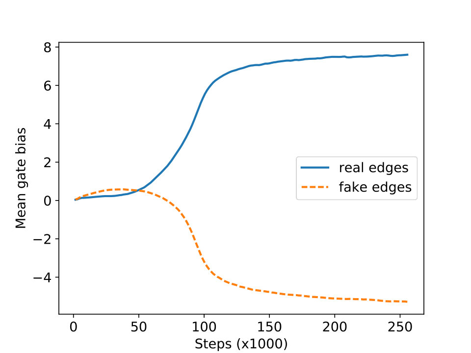 Figure 1
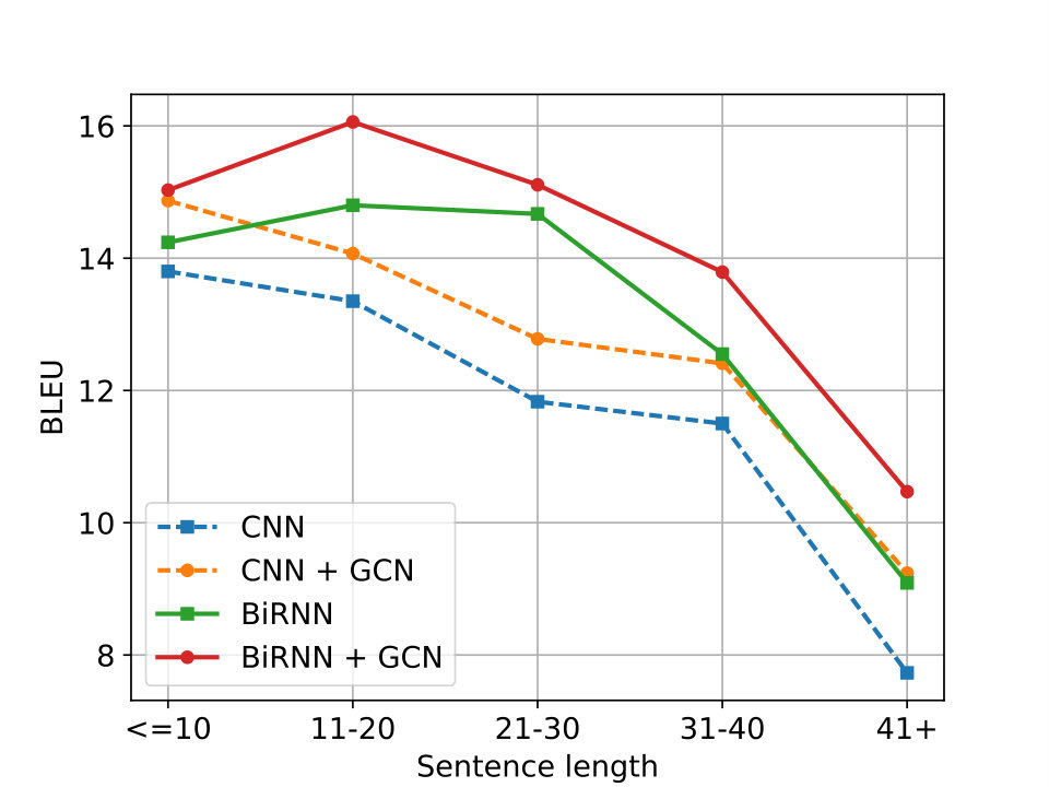 Figure 2
| Train | Val. | Test | |
|---|---|---|---|
| English-German | 226822 | 2169 | 2999 |
| English-German (full) | 4500966 | 2169 | 2999 |
| English-Czech | 181112 | 2656 | 2999 |
| Source | Target | |
|---|---|---|
| English-German | 37824 | 8099 (BPE) |
| English-German (full) | 50000 | 16000 (BPE) |
| English-Czech | 33786 | 8116 (BPE) |
| Kendall | BLEU1 | BLEU4 | |
|---|---|---|---|
| BoW | 0.3352 | 40.6 | 9.5 |
| + GCN | 0.3520 | 44.9 | 12.2 |
| CNN | 0.3601 | 42.8 | 12.6 |
| + GCN | 0.3777 | 44.7 | 13.7 |
| BiRNN | 0.3984 | 45.2 | 14.9 |
| + GCN | 0.4089 | 47.5 | 16.1 |
| BiRNN (full) | 0.5440 | 53.0 | 23.3 |
| + GCN | 0.5555 | 54.6 | 23.9 |
| Kendall | BLEU1 | BLEU4 | |
|---|---|---|---|
| BoW | 0.2498 | 32.9 | 6.0 |
| + GCN | 0.2561 | 35.4 | 7.5 |
| CNN | 0.2756 | 35.1 | 8.1 |
| + GCN | 0.2850 | 36.1 | 8.7 |
| BiRNN | 0.2961 | 36.9 | 8.9 |
| + GCN | 0.3046 | 38.8 | 9.6 |
| En-De | En-Cs | |||
|---|---|---|---|---|
| BLEU1 | BLEU4 | BLEU1 | BLEU4 | |
| BiRNN | 44.2 | 14.1 | 37.8 | 8.9 |
| + GCN (1L) | 45.0 | 14.1 | 38.3 | 9.6 |
| + GCN (2L) | 46.3 | 14.8 | 39.6 | 9.9 |
Peer Reviews
No public reviews on file for this paper yet. If you reviewed it on a platform where reviews are public (OpenReview, ICLR, NeurIPS, ICML), you can paste yours below so the community can read it here.
Videos
No videos yet. Explain this paper in a talk, walkthrough, or lecture? Add one.
Graph Convolutional Encoders
for Syntax-aware Neural Machine Translation
Jasmijn Bastings1 Ivan Titov1,2 Wilker Aziz1
Diego Marcheggiani1 Khalil Sima’an1
1ILLC, University of Amsterdam 2ILCC, University of Edinburgh
{bastings,titov,w.aziz,marcheggiani,k.simaan}@uva.nl
Abstract
We present a simple and effective approach to incorporating syntactic structure into neural attention-based encoder-decoder models for machine translation. We rely on graph-convolutional networks (GCNs), a recent class of neural networks developed for modeling graph-structured data. Our GCNs use predicted syntactic dependency trees of source sentences to produce representations of words (i.e. hidden states of the encoder) that are sensitive to their syntactic neighborhoods. GCNs take word representations as input and produce word representations as output, so they can easily be incorporated as layers into standard encoders (e.g., on top of bidirectional RNNs or convolutional neural networks). We evaluate their effectiveness with English-German and English-Czech translation experiments for different types of encoders and observe substantial improvements over their syntax-agnostic versions in all the considered setups.
1 Introduction
Neural machine translation (NMT) is one of success stories of deep learning in natural language processing, with recent NMT systems outperforming traditional phrase-based approaches on many language pairs Sennrich et al. (2016a). State-of-the-art NMT systems rely on sequential encoder-decoders Sutskever et al. (2014); Bahdanau et al. (2015) and lack any explicit modeling of syntax or any hierarchical structure of language. One potential reason for why we have not seen much benefit from using syntactic information in NMT is the lack of simple and effective methods for incorporating structured information in neural encoders, including RNNs. Despite some successes, techniques explored so far either incorporate syntactic information in NMT models in a relatively indirect way (e.g., multi-task learning Luong et al. (2015a); Nadejde et al. (2017); Eriguchi et al. (2017); Hashimoto and Tsuruoka (2017)) or may be too restrictive in modeling the interface between syntax and the translation task (e.g., learning representations of linguistic phrases Eriguchi et al. (2016)). Our goal is to provide the encoder with access to rich syntactic information but let it decide which aspects of syntax are beneficial for MT, without placing rigid constraints on the interaction between syntax and the translation task. This goal is in line with claims that rigid syntactic constraints typically hurt MT Zollmann and Venugopal (2006); Smith and Eisner (2006); Chiang (2010), and, though these claims have been made in the context of traditional MT systems, we believe they are no less valid for NMT.
Attention-based NMT systems Bahdanau et al. (2015); Luong et al. (2015b) represent source sentence words as latent-feature vectors in the encoder and use these vectors when generating a translation. Our goal is to automatically incorporate information about syntactic neighborhoods of source words into these feature vectors, and, thus, potentially improve quality of the translation output. Since vectors correspond to words, it is natural for us to use dependency syntax. Dependency trees (see Figure 1) represent syntactic relations between words: for example, monkey is a subject of the predicate eats, and banana is its object.
In order to produce syntax-aware feature representations of words, we exploit graph-convolutional networks (GCNs) Duvenaud et al. (2015); Defferrard et al. (2016); Kearnes et al. (2016); Kipf and Welling (2016). GCNs can be regarded as computing a latent-feature representation of a node (i.e. a real-valued vector) based on its -th order neighborhood (i.e. nodes at most hops aways from the node) Gilmer et al. (2017). They are generally simple and computationally inexpensive. We use Syntactic GCNs, a version of GCN operating on top of syntactic dependency trees, recently shown effective in the context of semantic role labeling Marcheggiani and Titov (2017).
Since syntactic GCNs produce representations at word level, it is straightforward to use them as encoders within the attention-based encoder-decoder framework. As NMT systems are trained end-to-end, GCNs end up capturing syntactic properties specifically relevant to the translation task. Though GCNs can take word embeddings as input, we will see that they are more effective when used as layers on top of recurrent neural network (RNN) or convolutional neural network (CNN) encoders Gehring et al. (2016), enriching their states with syntactic information. A comparison to RNNs is the most challenging test for GCNs, as it has been shown that RNNs (e.g., LSTMs) are able to capture certain syntactic phenomena (e.g., subject-verb agreement) reasonably well on their own, without explicit treebank supervision Linzen et al. (2016); Shi et al. (2016). Nevertheless, GCNs appear beneficial even in this challenging set-up: we obtain +1.2 and +0.7 BLEU point improvements from using syntactic GCNs on top of bidirectional RNNs for English-German and English-Czech, respectively.
In principle, GCNs are flexible enough to incorporate any linguistic structure as long as they can be represented as graphs (e.g., dependency-based semantic-role labeling representations Surdeanu et al. (2008), AMR semantic graphs Banarescu et al. (2012) and co-reference chains). For example, unlike recursive neural networks Socher et al. (2013), GCNs do not require the graphs to be trees. However, in this work we solely focus on dependency syntax and leave more general investigation for future work.
Our main contributions can be summarized as follows:
- •
we introduce a method for incorporating structure into NMT using syntactic GCNs;
- •
we show that GCNs can be used along with RNN and CNN encoders;
- •
we show that incorporating structure is beneficial for machine translation on English-Czech and English-German.
2 Background
Notation.
We use for vectors, for a sequence of vectors, and for matrices. The -th value of vector is denoted by . We use for vector concatenation.
2.1 Neural Machine Translation
In NMT Kalchbrenner and Blunsom (2013); Sutskever et al. (2014); Cho et al. (2014b), given example translation pairs from a parallel corpus, a neural network is trained to directly estimate the conditional distribution of translating a source sentence (a sequence of words) into a target sentence . NMT models typically consist of an encoder, a decoder and some method for conditioning the decoder on the encoder, for example, an attention mechanism. We will now briefly describe the components that we use in this paper.
2.1.1 Encoders
An encoder is a function that takes as input the source sentence and produces a representation encoding its semantic content. We describe recurrent, convolutional and bag-of-words encoders.
Recurrent.
Recurrent neural networks (RNNs) Elman (1990) model sequential data. They receive one input vector at each time step and update their hidden state to summarize all inputs up to that point. Given an input sequence of word embeddings an RNN is defined recursively as follows:
[TABLE]
where is a nonlinear function such as an LSTM Hochreiter and Schmidhuber (1997) or a GRU Cho et al. (2014b). We will use the function RNN as an abstract mapping from an input sequence to final hidden state , regardless of the used nonlinearity. To not only summarize the past of a word, but also its future, a bidirectional RNN Schuster and Paliwal (1997); Irsoy and Cardie (2014) is often used. A bidirectional RNN reads the input sentence in two directions and then concatenates the states for each time step:
[TABLE]
where and are the forward and backward RNNs, respectively. For further details we refer to the encoder of Bahdanau et al. (2015).
Convolutional.
Convolutional Neural Networks (CNNs) apply a fixed-size window over the input sequence to capture the local context of each word Gehring et al. (2016). One advantage of this approach over RNNs is that it allows for fast parallel computation, while sacrificing non-local context. To remedy the loss of context, multiple CNN layers can be stacked. Formally, given an input sequence , we define a CNN as follows:
[TABLE]
where is a nonlinear function, typically a linear transformation followed by ReLU, and is the size of the window.
Bag-of-Words.
In a bag-of-words (BoW) encoder every word is simply represented by its word embedding. To give the decoder some sense of word position, position embeddings (PE) may be added. There are different strategies for defining position embeddings, and in this paper we choose to learn a vector for each absolute word position up to a certain maximum length. We then represent the -th word in a sequence as follows:
[TABLE]
where is the word embedding and is the t-th position embedding.
2.1.2 Decoder
A decoder produces the target sentence conditioned on the representation of the source sentence induced by the encoder. In Bahdanau et al. (2015) the decoder is implemented as an RNN conditioned on an additional input , the context vector, which is dynamically computed at each time step using an attention mechanism.
The probability of a target word is now a function of the decoder RNN state, the previous target word embedding, and the context vector. The model is trained end-to-end for maximum log likelihood of the next target word given its context.
2.2 Graph Convolutional Networks
We will now describe the Graph Convolutional Networks (GCNs) of Kipf and Welling (2016). For a comprehensive overview of alternative GCN architectures see Gilmer et al. (2017).
A GCN is a multilayer neural network that operates directly on a graph, encoding information about the neighborhood of a node as a real-valued vector. In each GCN layer, information flows along edges of the graph; in other words, each node receives messages from all its immediate neighbors. When multiple GCN layers are stacked, information about larger neighborhoods gets integrated. For example, in the second layer, a node will receive information from its immediate neighbors, but this information already includes information from their respective neighbors. By choosing the number of GCN layers, we regulate the distance the information travels: with layers a node receives information from neighbors at most hops away.
Formally, consider an undirected graph , where is a set of nodes, and is a set of edges. Every node is assumed to be connected to itself, i.e. Now, let be a matrix containing all nodes with their features, where is the dimensionality of the feature vectors. In our case, will contain word embeddings, but in general it can contain any kind of features. For a 1-layer GCN, the new node representations are computed as follows:
[TABLE]
where is a weight matrix and a bias vector.111We dropped the normalization factor used by Kipf and Welling (2016), as it is not used in syntactic GCNs of Marcheggiani and Titov (2017). is an activation function, e.g. a ReLU. is the set of neighbors of , which we assume here to always include itself. As stated before, to allow information to flow over multiple hops, we need to stack GCN layers. The recursive computation is as follows:
[TABLE]
where indexes the layer, and .
2.3 Syntactic GCNs
Marcheggiani and Titov (2017) generalize GCNs to operate on directed and labeled graphs.222For an alternative approach to integrating labels and directions, see applications of GCNs to statistical relation learning Schlichtkrull et al. (2017). This makes it possible to use linguistic structures such as dependency trees, where directionality and edge labels play an important role. They also integrate edge-wise gates which let the model regulate contributions of individual dependency edges. We will briefly describe these modifications.
Directionality.
In order to deal with directionality of edges, separate weight matrices are used for incoming and outgoing edges. We follow the convention that in dependency trees heads point to their dependents, and thus outgoing edges are used for head-to-dependent connections, and incoming edges are used for dependent-to-head connections. Modifying the recursive computation for directionality, we arrive at:
[TABLE]
where selects the weight matrix associated with the directionality of the edge connecting and (i.e. for -to-, for -to-, and for -to-). Note that self loops are modeled separately,
so there are now three times as many parameters as in a non-directional GCN.
Labels.
Making the GCN sensitive to labels is straightforward given the above modifications for directionality. Instead of using separate matrices for each direction, separate matrices are now defined for each direction and label combination:
[TABLE]
where we incorporate the directionality of an edge directly in its label.
Importantly, to prevent over-parametrization, only bias terms are made label-specific, in other words: . The resulting syntactic GCN is illustrated in Figure 2 (shown on top of a CNN, as we will explain in the subsequent section).
Edge-wise gating.
Syntactic GCNs also include gates, which can down-weight the contribution of individual edges. They also allow the model to deal with noisy predicted structure, i.e. to ignore potentially erroneous syntactic edges. For each edge, a scalar gate is calculated as follows:
[TABLE]
where is the logistic sigmoid function, and and are learned parameters for the gate. The computation becomes:
[TABLE]
3 Graph Convolutional Encoders
In this work we focus on exploiting structural information on the source side, i.e. in the encoder. We hypothesize that using an encoder that incorporates syntax will lead to more informative representations of words, and that these representations, when used as context vectors by the decoder, will lead to an improvement in translation quality. Consequently, in all our models, we use the decoder of Bahdanau et al. (2015) and keep this part of the model constant. As is now common practice, we do not use a maxout layer in the decoder, but apart from this we do not deviate from the original definition. In all models we make use of GRUs Cho et al. (2014b) as our RNN units.
Our models vary in the encoder part, where we exploit the power of GCNs to induce syntactically-aware representations. We now define a series of encoders of increasing complexity.
BoW + GCN.
In our first and simplest model, we propose a bag-of-words encoder (with position embeddings, see §2.1.1), with a GCN on top. In other words, inputs are a sum of embeddings of a word and its position in a sentence. Since the original BoW encoder captures the linear ordering information only in a very crude way (through the position embeddings), the structural information provided by GCN should be highly beneficial.
Convolutional + GCN.
In our second model, we use convolutional neural networks to learn word representations. CNNs are fast, but by definition only use a limited window of context. Instead of the approach used by Gehring et al. (2016) (i.e. stacking multiple CNN layers on top of each other), we use a GCN to enrich the one-layer CNN representations. Figure 2 shows this model. Note that, while the figure shows a CNN with a window size of 3, we will use a larger window size of 5 in our experiments. We expect this model to perform better than BoW + GCN, because of the additional local context captured by the CNN.
BiRNN + GCN.
In our third and most powerful model, we employ bidirectional recurrent neural networks. In this model, we start by encoding the source sentence using a BiRNN (i.e. BiGRU), and use the resulting hidden states as input to a GCN. Instead of relying on linear order only, the GCN will allow the encoder to ‘teleport’ over parts of the input sentence, along dependency edges, connecting words that otherwise might be far apart. The model might not only benefit from this teleporting capability however; also the nature of the relations between words (i.e. dependency relation types) may be useful, and the GCN exploits this information (see §2.3 for details).
This is the most challenging setup for GCNs, as RNNs have been shown capable of capturing at least some degree of syntactic information without explicit supervision Linzen et al. (2016), and hence they should be hard to improve on by incorporating treebank syntax.
Marcheggiani and Titov (2017) did not observe improvements from using multiple GCN layers in semantic role labeling. However, we do expect that propagating information from further in the tree should be beneficial in principle. We hypothesize that the first layer is the most influential one, capturing most of the syntactic context, and that additional layers only modestly modify the representations. To ease optimization, we add a residual connection He et al. (2016) between the GCN layers, when using more than one layer.
4 Experiments
Experiments are performed using the Neural Monkey toolkit333https://github.com/ufal/neuralmonkey Helcl and Libovický (2017), which implements the model of Bahdanau et al. (2015) in TensorFlow. We use the Adam optimizer Kingma and Ba (2015) with a learning rate of 0.001 (0.0002 for CNN models).444Like Gehring et al. (2016) we note that Adam is too aggressive for CNN models, hence we use a lower learning rate. The batch size is set to 80. Between layers we apply dropout with a probability of 0.2, and in experiments with GCNs555GCN code at https://github.com/bastings/neuralmonkey we use the same value for edge dropout. We train for 45 epochs, evaluating the BLEU performance of the model every epoch on the validation set. For testing, we select the model with the highest validation BLEU. L2 regularization is used with a value of . All the model selection (incl. hyperparameter selections) was performed on the validation set. In all experiments we obtain translations using a greedy decoder, i.e. we select the output token with the highest probability at each time step.
We will describe an artificial experiment in §4.1 and MT experiments in §4.2.
4.1 Reordering artificial sequences
Our goal here is to provide an intuition for the capabilities of GCNs. We define a reordering task where randomly permuted sequences need to be put back into the original order. We encode the original order using edges, and test if GCNs can successfully exploit them. Note that this task is not meant to provide a fair comparison to RNNs. The input (besides the edges) simply does not carry any information about the original ordering, so RNNs cannot possibly solve this task.
Data.
From a vocabulary of 26 types, we generate random sequences of 3-10 tokens. We then randomly permute them, pointing every token to its original predecessor with a label sampled from a set of 5 labels. Additionally, we point every token to an arbitrary position in the sequence with a label from a distinct set of 5 ‘fake’ labels. We sample 25000 training and 1000 validation sequences.
Model.
We use the BiRNN + GCN model, i.e. a bidirectional GRU with a 1-layer GCN on top. We use 32, 64 and 128 units for embeddings, GRU units and GCN layers, respectively.
Results.
After 6 epochs of training, the model learns to put permuted sequences back into order, reaching a validation BLEU of . Figure 3 shows that the mean values of the bias terms of gates (i.e. ) for real and fake edges are far apart, suggesting that the GCN learns to distinguish them. Interestingly, this illustrates why edge-wise gating is beneficial. A gate-less model would not understand which of the two outgoing arcs is fake and which is genuine, because only biases would then be label-dependent. Consequently, it would only do a mediocre job in reordering. Although using label-specific matrices would also help, this would not scale to the real scenario (see §2.3).
4.2 Machine Translation
Data.
For our experiments we use the En-De and En-Cs News Commentary v11 data from the WMT16 translation task.666http://www.statmt.org/wmt16/translation-task.html For En-De we also train on the full WMT16 data set. As our validation set and test set we use newstest2015 and newstest2016, respectively.
Pre-processing.
The English sides of the corpora are tokenized and parsed into dependency trees by SyntaxNet,777https://github.com/tensorflow/models/tree/master/syntaxnet using the pre-trained Parsey McParseface model.888The used dependency parses can be reproduced by using the syntaxnet/demo.sh shell script. The Czech and German sides are tokenized using the Moses tokenizer.999https://github.com/moses-smt/mosesdecoder Sentence pairs where either side is longer than 50 words are filtered out after tokenization.
Vocabularies.
For the English sides, we construct vocabularies from all words except those with a training set frequency smaller than three. For Czech and German, to deal with rare words and phenomena such as inflection and compounding, we learn byte-pair encodings (BPE) as described by Sennrich et al. (2016b). Given the size of our data set, and following Wu et al. (2016), we use 8000 BPE merges to obtain robust frequencies for our subword units (16000 merges for full data experiment). Data set statistics are summarized in Table 1 and vocabulary sizes in Table 2.
Hyperparameters.
We use 256 units for word embeddings, 512 units for GRUs (800 for En-De full data set experiment), and 512 units for convolutional layers (or equivalently, 512 ‘channels’). The dimensionality of the GCN layers is equivalent to the dimensionality of their input. We report results for 2-layer GCNs, as we find them most effective (see ablation studies below).
Baselines.
We provide three baselines, each with a different encoder: a bag-of-words encoder, a convolutional encoder with window size , and a BiRNN. See §2.1.1 for details.
Evaluation.
We report (cased) BLEU results Papineni et al. (2002) using multi-bleu, as well as Kendall reordering scores.101010See Stanojević and Sima’an (2015). TER Snover et al. (2006) and BEER Stanojević and Sima’an (2014) metrics, even though omitted due to space considerations, are consistent with the reported results.
4.2.1 Results
English-German.
Table 3 shows test results on English-German. Unsurprisingly, the bag-of-words baseline performs the worst. We expected the BoW+GCN model to make easy gains over this baseline, which is indeed what happens. The CNN baseline reaches a higher BLEU4 score than the BoW models, but interestingly its BLEU1 score is lower than the BoW+GCN model. The CNN+GCN model improves over the CNN baseline by +1.9 and +1.1 for BLEU1 and BLEU4, respectively. The BiRNN, the strongest baseline, reaches a BLEU4 of 14.9. Interestingly, GCNs still manage to improve the result by +2.3 BLEU1 and +1.2 BLEU4 points. Finally, we observe a big jump in BLEU4 by using the full data set and beam search (beam 12). The BiRNN now reaches 23.3, while adding a GCN achieves a score of 23.9.
English-Czech.
Table 4 shows test results on English-Czech. While it is difficult to obtain high absolute BLEU scores on this dataset, we can still see similar relative improvements. Again the BoW baseline scores worst, with the BoW+GCN easily beating that result. The CNN baseline scores BLEU4 of 8.1, but the CNN+GCN improves on that, this time by +1.0 and +0.6 for BLEU1 and BLEU4, respectively. Interestingly, BLEU1 scores for the BoW+GCN and CNN+GCN models are higher than both baselines so far. Finally, the BiRNN baseline scores a BLEU4 of 8.9, but it is again beaten by the BiRNN+GCN model with +1.9 BLEU1 and +0.7 BLEU4.
Effect of GCN layers.
How many GCN layers do we need? Every layer gives us an extra hop in the graph and expands the syntactic neighborhood of a word. Table 5 shows validation BLEU performance as a function of the number of GCN layers. For English-German, using a 1-layer GCN improves BLEU-1, but surprisingly has little effect on BLEU4. Adding an additional layer gives improvements on both BLEU1 and BLEU4 of +1.3 and +0.73, respectively. For English-Czech, performance increases with each added GCN layer.
Effect of sentence length.
We hypothesize that GCNs should be more beneficial for longer sentences: these are likely to contain long-distance syntactic dependencies which may not be adequately captured by RNNs but directly encoded in GCNs. To test this, we partition the validation data into five buckets and calculate BLEU for each of them. Figure 4 shows that GCN-based models outperform their respective baselines rather uniformly across all buckets. This is a surprising result. One explanation may be that syntactic parses are noisier for longer sentences, and this prevents us from obtaining extra improvements with GCNs.
Discussion.
Results suggest that the syntax-aware representations provided by GCNs consistently lead to improved translation performance as measured by BLEU4 (as well as TER and BEER). Consistent gains in terms of Kendall tau and BLEU1 indicate that improvements correlate with better word order and lexical/BPE selection, two phenomena that depend crucially on syntax.
5 Related Work
We review various accounts to syntax in NMT as well as other convolutional encoders.
Syntactic features and/or constraints.
Sennrich and Haddow (2016) embed features such as POS-tags, lemmas and dependency labels and feed these into the network along with word embeddings. Eriguchi et al. (2016) parse English sentences with an HPSG parser and use a Tree-LSTM to encode the internal nodes of the tree. In the decoder, word and node representations compete under the same attention mechanism. Stahlberg et al. (2016) use a pruned lattice from a hierarchical phrase-based model (hiero) to constrain NMT. Hiero trees are not syntactically-aware, but instead constrained by symmetrized word alignments. Aharoni and Goldberg (2017) propose neural string-to-tree by predicting linearized parse trees.
Multi-task Learning.
Sharing NMT parameters with a syntactic parser is a popular approach to obtaining syntactically-aware representations. Luong et al. (2015a) predict linearized constituency parses as an additional task. Eriguchi et al. (2017) multi-task with a target-side RNNG parser Dyer et al. (2016) and improve on various language pairs with English on the target side. Nadejde et al. (2017) multi-task with CCG tagging, and also integrate syntax on the target side by predicting a sequence of words interleaved with CCG supertags.
Latent structure.
Hashimoto and Tsuruoka (2017) add a syntax-inspired encoder on top of a BiLSTM layer. They encode source words as a learned average of potential parents emulating a relaxed dependency tree. While their model is trained purely on translation data, they also experiment with pre-training the encoder using treebank annotation and report modest improvements on English-Japanese. Yogatama et al. (2016) introduce a model for language understanding and generation that composes words into sentences by inducing unlabeled binary bracketing trees.
Convolutional encoders.
Gehring et al. (2016) show that CNNs can be competitive to BiRNNs when used as encoders. To increase the receptive field of a word’s context they stack multiple CNN layers. Kalchbrenner et al. (2016) use convolution in both the encoder and the decoder; they make use of dilation to increase the receptive field. In contrast to both approaches, we use a GCN informed by dependency structure to increase it. Finally, Cho et al. (2014a) propose a recursive convolutional neural network which builds a tree out of the word leaf nodes, but which ends up compressing the source sentence in a single vector.
6 Conclusions
We have presented a simple and effective approach to integrating syntax into neural machine translation models and have shown consistent BLEU4 improvements for two challenging language pairs: English-German and English-Czech. Since GCNs are capable of encoding any kind of graph-based structure, in future work we would like to go beyond syntax, by using semantic annotations such as SRL and AMR, and co-reference chains.
Acknowledgments
We would like to thank Michael Schlichtkrull and Thomas Kipf for their suggestions and comments. This work was supported by the European Research Council (ERC StG BroadSem 678254) and the Dutch National Science Foundation (NWO VIDI 639.022.518, NWO VICI 277-89-002).
The reference list from the paper itself. Each links out to its DOI / PubMed record.
- 1Aharoni and Goldberg (2017) Roee Aharoni and Yoav Goldberg. 2017. Towards String-to-Tree Neural Machine Translation . Ar Xiv e-prints .
- 2Bahdanau et al. (2015) Dzmitry Bahdanau, Kyunghyun Cho, and Yoshua Bengio. 2015. Neural Machine Translation by Jointly Learning to Align and Translate . In Proceedings of the International Conference on Learning Representations (ICLR) .
- 3Banarescu et al. (2012) Laura Banarescu, Claire Bonial, Shu Cai, Madalina Georgescu, Kira Griffitt, Ulf Hermjakob, Kevin Knight, Philipp Koehn, Martha Palmer, and Nathan Schneider. 2012. Abstract meaning representation (amr) 1.0 specification. In Conference on Empirical Methods in Natural Language Processing , pages 1533–1544.
- 4Chiang (2010) David Chiang. 2010. Learning to translate with source and target syntax . In Proceedings of the 48th Annual Meeting of the Association for Computational Linguistics , pages 1443–1452, Uppsala, Sweden. Association for Computational Linguistics.
- 5Cho et al. (2014 a) Kyung Hyun Cho, Bart van Merrienboer, Dzmitry Bahdanau, and Yoshua Bengio. 2014 a. On the Properties of Neural Machine Translation: Encoder-Decoder Approaches . In SSST-8, Eighth Workshop on Syntax, Semantics and Structure in Statistical Translation , volume abs/1409.1259, pages 103–111.
- 6Cho et al. (2014 b) Kyunghyun Cho, Bart van Merrienboer, Caglar Gulcehre, Dzmitry Bahdanau, Fethi Bougares, Holger Schwenk, and Yoshua Bengio. 2014 b. Learning Phrase Representations using RNN Encoder–Decoder for Statistical Machine Translation . In Proceedings of the 2014 Conference on Empirical Methods in Natural Language Processing (EMNLP) , pages 1724–1734, Doha, Qatar. Association for Computational Linguistics.
- 7Defferrard et al. (2016) Michaël Defferrard, Xavier Bresson, and Pierre Vandergheynst. 2016. Convolutional neural networks on graphs with fast localized spectral filtering . In Advances in Neural Information Processing Systems 29: Annual Conference on Neural Information Processing Systems 2016, December 5-10, 2016, Barcelona, Spain , pages 3837–3845.
- 8Duvenaud et al. (2015) David K Duvenaud, Dougal Maclaurin, Jorge Iparraguirre, Rafael Bombarell, Timothy Hirzel, Alán Aspuru-Guzik, and Ryan P Adams. 2015. Convolutional networks on graphs for learning molecular fingerprints. In Advances in neural information processing systems , pages 2224–2232.