Small and Strong Formulations for Unions of Convex Sets from the Cayley Embedding
Juan Pablo Vielma

TL;DR
This paper introduces a novel geometric technique based on Cayley embeddings to create small, strong mixed-integer programming formulations for unions of convex sets without auxiliary continuous variables, improving computational efficiency.
Contribution
It develops a new geometric approach that generalizes Cayley embeddings, enabling the construction of strong, compact formulations for convex disjunctive constraints without auxiliary variables.
Findings
The technique recovers all known strong formulations without auxiliary variables.
It produces smaller and stronger formulations for a wide range of disjunctive constraints.
The approach inherits geometric properties from the Cayley embedding, ensuring robustness.
Abstract
There is often a significant trade-off between formulation strength and size in mixed integer programming (MIP). When modeling convex disjunctive constraints (e.g. unions of convex sets), adding auxiliary continuous variables can sometimes help resolve this trade-off. However, standard formulations that use such auxiliary continuous variables can have a worse-than-expected computational effectiveness, which is often attributed precisely to these auxiliary continuous variables. For this reason, there has been considerable interest in constructing strong formulations that do not use continuous auxiliary variables. We introduce a technique to construct formulations without these detrimental continuous auxiliary variables. To develop this technique we introduce a natural non-polyhedral generalization of the Cayley embedding of a family of polytopes and show it inherits many geometric…
Click any figure to enlarge with its caption.
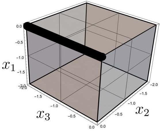 Figure 1
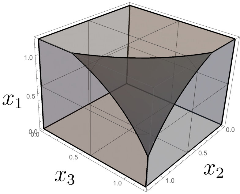 Figure 2
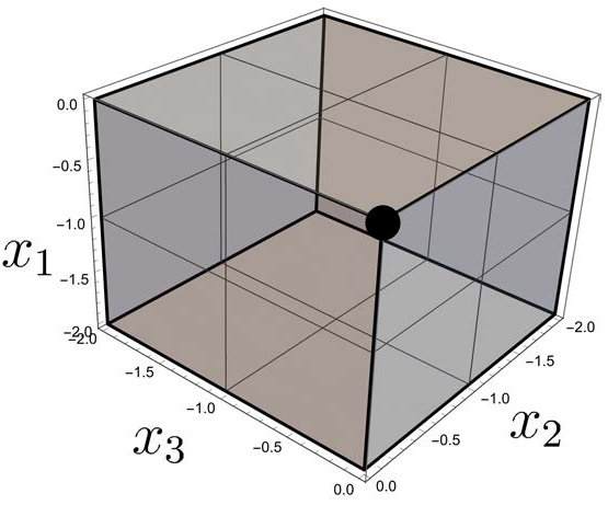 Figure 3
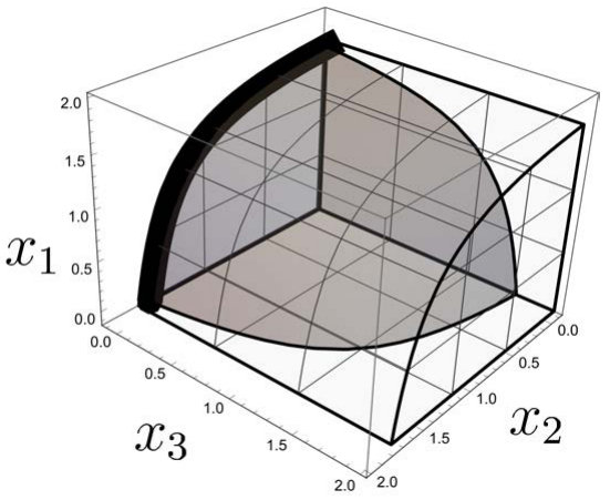 Figure 4
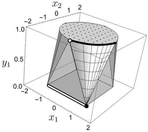 Figure 5
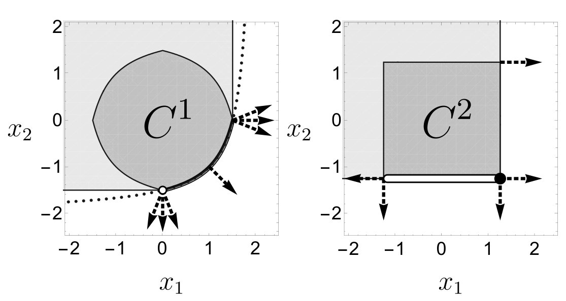 Figure 6
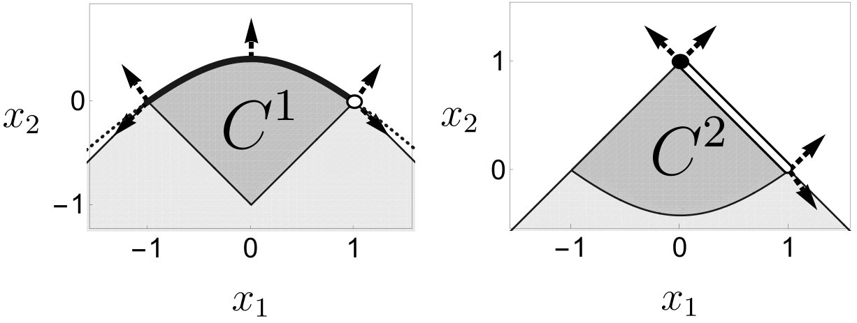 Figure 7
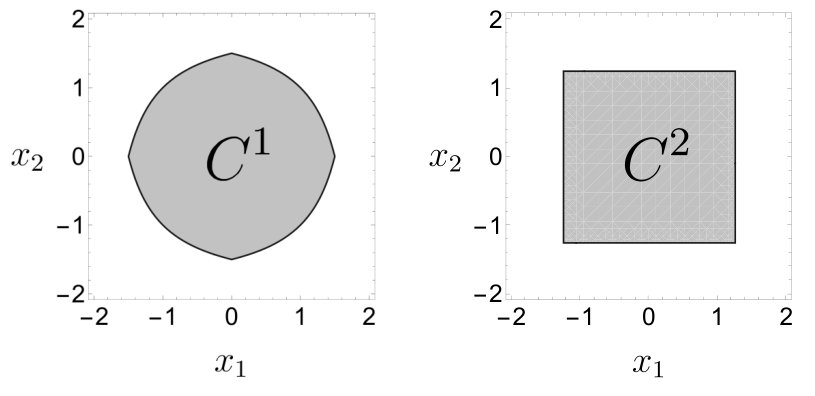 Figure 8
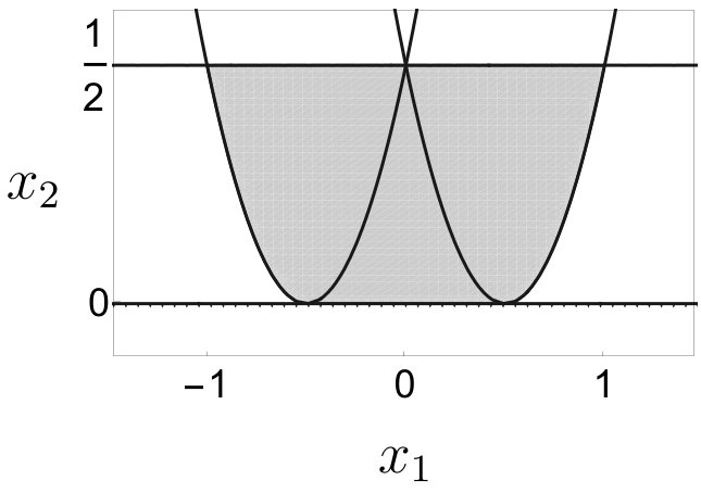 Figure 9
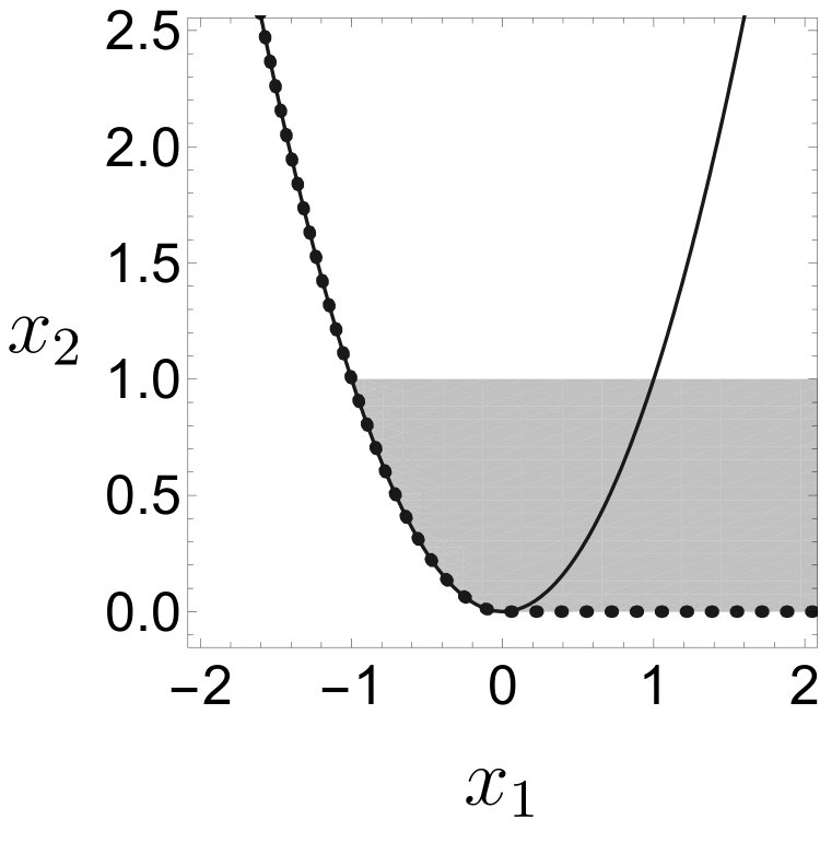 Figure 10
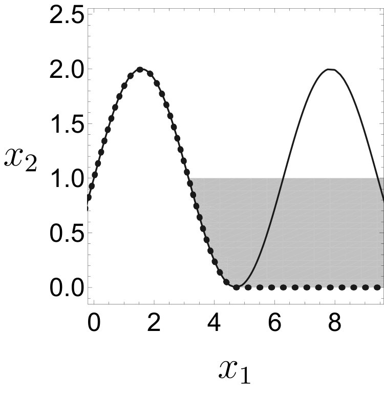 Figure 11
 Figure 12
Peer Reviews
No public reviews on file for this paper yet. If you reviewed it on a platform where reviews are public (OpenReview, ICLR, NeurIPS, ICML), you can paste yours below so the community can read it here.
Videos
No videos yet. Explain this paper in a talk, walkthrough, or lecture? Add one.
∎
11institutetext: Sloan School of Management, Massachusetts Institute of Technology, Cambridge MA 02139, USA,
11email: [email protected]
Small and Strong Formulations for Unions of Convex Sets from the Cayley Embedding
Juan Pablo Vielma
(Received: date / Accepted: date)
Abstract
There is often a significant trade-off between formulation strength and size in mixed integer programming (MIP). When modeling convex disjunctive constraints (e.g. unions of convex sets), adding auxiliary continuous variables can sometimes help resolve this trade-off. However, standard formulations that use such auxiliary continuous variables can have a worse-than-expected computational effectiveness, which is often attributed precisely to these auxiliary continuous variables. For this reason, there has been considerable interest in constructing strong formulations that do not use continuous auxiliary variables. We introduce a technique to construct formulations without these detrimental continuous auxiliary variables. To develop this technique we introduce a natural non-polyhedral generalization of the Cayley embedding of a family of polytopes and show it inherits many geometric properties of the original embedding. We then show how the associated formulation technique can be used to construct small and strong formulation for a wide range of disjunctive constraints. In particular, we show it can recover and generalize all known strong formulations without continuous auxiliary variables.
Keywords:
Mixed integer nonlinear programming; Mixed integer programming formulations; Disjunctive constraints
1 Introduction
Mixed integer programming (MIP) adds integrality requirements to a continuous optimization problem, which is often referred to as the continuous relaxation of the MIP problem. MIP problems with a convex continuous relaxation often arise from the need to model disjunctive constraint of the form where is a family of closed convex sets. The two main classes of formulations for these constraints are the so-called Big-M and convex hull formulations. Big-M formulations are simple and small, but their continuous relaxations usually yield weak bounds, which can hinder the performance of branch-and-bound based algorithms. In contrast, the convex hull formulation yields the best possible relaxation bounds for a single disjunctive constraint and normally yields strong bounds for problems with multiple constraints. Unfortunately, while convex hull formulations are only moderately larger than Big-M formulations, their computational performance is usually much worse. The folklore attributes this poor performance to certain continuous auxiliary variables used by the convex hull formulation. This has prompted significant interest on techniques to project out such variables (i.e. eliminate them without decreasing the formulation’s strength). The resulting formulations can provide a significant computational advantage, but existing techniques are limited to very specific structures (e.g. see balas88 ; blair90 ; jeroslow88 ; Embedding ; DBLP:journals/mp/VielmaN11 for polyhedra and lodi15 ; gunluk2010perspective ; Hijazi ; mohit1 ; mohit2 for non-polyhedral sets). In this paper we introduce a technique to project out the detrimental auxiliary variables for a wide range of disjunctive constraints. In particular, the technique can be used to recover, and generalize all known results that use binary variables that add to one (e.g. excluding the logarithmic formulation from Embedding ; DBLP:journals/mp/VielmaN11 ).
Our technique is based on a geometric characterization of the projection of the convex hull formulation that connects it to a natural non-polyhedral generalization of an object known as the Cayley embedding of a family of polytopes. To obtain this characterization we generalize to the non-polyhedral setting some known properties of the Cayley embedding and use it to obtain a valid formulation of the disjunctive constraint. We then give simple sufficient conditions for this formulation to be equal to the projection of the convex hull formulation. Using these conditions we then recover and generalize all known techniques to project the convex hull formulation. We also provide precise necessary and sufficient conditions to obtain the projection and comment on the practical implementation of the formulations. In particular, we evaluate the representation of the projection from an algebraic geometry perspective.
The paper is organized as follows. In Section 2 we introduce a geometric abstraction that unifies all known formulations in a common framework. In Section 3 we introduce the geometric characterization and describe the projected convex hull formulation for two simple cases. In Section 4 we present the generalized properties of the Cayley embedding and the simple sufficient conditions. We then use these conditions to recover and generalize all existing formulations in Section 5. In particular, we give guidance on how to apply the technique, comment on its practical implementation and present the algebraic geometry result. Finally, in Section 6 we give detailed necessary and sufficient conditions for the technique. Omitted proofs are included in Section 8.
We use the following notation. For a function we let its epigraph be . For a set we denote its topological closure, its convex hull, its conic hull and its affine hull by , , and . For a closed convex set we denote its recession cone by and the set containing all its extreme points by . We let \left\llbracket k\right\rrbracket:=\left\{1,\ldots,k\right\}, be the -th canonical vector, be the all ones vector and be the all zeros vector (the specific dimension will be apparent from the context). For a closed convex cone we let be its polar cone. Finally, we let be the set of integers.
2 MIP formulations for unions of convex sets
Definition 1
Let be a finite family of closed convex sets and be a closed convex set. We say is a MIP formulation of if and only if
[TABLE]
We refer to as the continuous relaxation of the MIP formulation and say the formulation is ideal if and only if for any minimal face of and we have .
Existing formulations depend on specific set-representations. For instance, Balas, Jeroslow and Lowe give linear MIP formulations for polyhedra (e.g. (Mixed-Integer-Linear-Programming-Formulation-Techniques, , Section 5)), Ben-Tal, Helton, Nemirovski and Nie give conic MIP formulations for conic representable sets ben2001lectures ; Helton and Ceria, Merhotra, Soares and Stubs give perspective function formulations for function level sets springerlink:10.1007/s101070050106 ; springerlink:10.1007/s101070050103 . To abstract the representation we use the following properties of the gauge of a convex set (e.g. hiriart-lemarechal-2001 ).
Lemma 1
Let be a closed convex set with and be the gauge function of given by . Then the following properties hold.
- •
If for all , then .
- •
The gauge function is convex and positively homogeneous.
- •
We have that and .
Furthermore, if is a closed convex set and , then
[TABLE]
Using gauge functions we can construct a generic versions of standard formulations for convex sets that satisfy the following assumption.
Definition 2
We say if and only if is a non-empty closed convex set for all i\in\left\llbracket k\right\rrbracket and for all i,j\in\left\llbracket k\right\rrbracket.
Theorem 2.1 ()
Let and be such that for all i\in\left\llbracket k\right\rrbracket, then an ideal formulation for is given by
[TABLE]
In particular, if for all i\in\left\llbracket k\right\rrbracket, then the continuous relaxation of (2) is line-free and all of its extreme points have integral components.
The proof of Theorem 2.1 is analogous to existing formulations, but for completeness we include a proof in Section 8.1.
A key to obtain the relatively simple and small ideal formulation (2) is the use of the copies of the original variables . Unfortunately, these variable copies induce a block structure that the MIP folklore identifies as a source of the worse-than-expected computational performance of formulation (2). For this reason, simpler Big-M formulations are often preferred in practice, even though they usually fail to be ideal. We can abstract the specific structure of such Big-M formulations using gauge functions as follows.
Theorem 2.2 ()
Let and be such that for all i\in\left\llbracket k\right\rrbracket, and be such that for all i\in\left\llbracket k\right\rrbracket and for all i,j\in\left\llbracket k\right\rrbracket. Then a formulation for is given by
[TABLE]
The strength of this formulation depended on with the strongest formulation being obtained for the smallest valid coefficients.
The abstraction provided by the use of gauge functions allow us to focus on the geometric structure of the formulations. However, it does not provide an explicit representation of the formulations that can be easily fed to a MIP solver. Fortunately, we can use known properties of gauge functions to obtain practical representation of various classes and recover existing formulations.
Lemma 2 ()
Let be closed and convex with and be a closed convex cone. Then if and only if and . In particular,
If for a closed convex cone , matrices and , and vector , then , 2. 2.
if is a closed convex function, is the closure of the perspective function of , and , then , 3. 3.
if , then , and 4. 4.
If then, .
The following example illustrates Lemma 2 and Theorems 2.1 and 2.2.
Example 1
Let and be the sets depicted in Figure 1. Using standard conic representability results for the cone (e.g. ben2001lectures ) we have
[TABLE]
Using Lemma 2 we have if and only if
[TABLE]
Similarly if and only if -\left(5/4\right)y\leq x_{j}\leq\left(5/4\right)y\quad\forall j\in\left\llbracket 2\right\rrbracket. Then Theorem 2.1 yields the ideal formulation for given by
[TABLE]
Alternatively, we can use Theorem 2.2 to obtain the formulation given by
[TABLE]
The smallest Big-M values that make this formulation valid are and . Unfortunately, we can check that for all the point with and is an extreme point of the continuous relaxation of (5) with fractional components. Furthermore, for all .∎
An ideal formulation without the variable copies can be obtained by projecting (2) onto the the and variables, but characterizing such projection can be challenging. However, an effective characterization can lead to significant computational improvements lodi15 ; gunluk2010perspective ; Hijazi ; Embedding ; DBLP:journals/mp/VielmaN11 . Unfortunately, there are only few general techniques to obtain these characterizations. One of the most general results by Balas, Blair and Jeroslow balas88 ; blair90 ; jeroslow88 considers unions of polyhedra with a common geometric structure (See Proposition 5.1 in Section 5.1). In contrast, non-polyhedral results require more structure and fall into two classes. The first class considers convex sets contained in orthogonal spaces mohit2 and can be stated in our gauge notation as follows.
Theorem 2.3 (mohit2 )
Let , be a finite family of compact convex sets in and be disjoint sets such that \bigcup_{i=1}^{k}J_{i}=\left\llbracket n\right\rrbracket and for all i\in\left\llbracket k\right\rrbracket we have and C^{i}\subseteq\left\{x\in\mathbb{R}^{n}\,:\,x_{j}=0\quad\forall j\in\left\llbracket n\right\rrbracket\setminus J_{i}\right\}. Then an ideal formulation for is given by
[TABLE]
where for and J\subseteq\left\llbracket n\right\rrbracket we let be such that if and otherwise.
The second class considers sets with certain monotonicity properties and generalizes “on/off” constraints gunluk2010perspective ; lodi15 ; Hijazi .
Theorem 2.4 (lodi15 ; Hijazi )
Let be a closed convex sets such that and . Furthermore, for each i\in\left\llbracket 2\right\rrbracket, let and C^{i}:=\left\{x\in G^{i}\,:\,l_{j}^{i}\leq x_{j}\leq u_{j}^{i}\quad\forall j\in\left\llbracket n\right\rrbracket\right\} be such that and for all j\in\left\llbracket n\right\rrbracket, and . Then an ideal formulation for is given by
[TABLE]
The most general known version of this result (e.g. Theorem 4 in lodi15 ) is obtained by combining Theorem 2.4 with Lemma 2 and noting that the result is still valid if we flip or mirror the axes of the variables. In fact, Theorems 2.4 and 2.3 can also be easily extended further by combining formulation (7) and any orthogonal transformation of the variables (i.e. axis flip plus rotation).
3 Ideal Formulations without Variable Copies
To construct the projection of formulation (2) onto the and variables we use a geometric characterization introduced in Embedding for the polyhedral setting. This characterization is based on the Cayley trick or Cayley Embedding, which is used to study Minkowski sums of polyhedra (e.g. caytrick ; karavelas2013maximum ; WeibelPhd ). The characterization in Embedding uses a generalization of the Cayley Embedding to consider alternative uses of [math]- variables (beyond the variables that add to one used in (2)). However, for simplicity we only generalize the standard version to the non-polyhedral setting through the following result we prove in Section 8.1.
Proposition 1 ()
Let and , where is the i-th -dimensional unit vector. Then
* is a closed convex set and ,* 2. 2.
* is the projection of the continuous relaxation of (2), and* 3. 3.
* is an ideal formulation of .*
Proposition 1 reduces the construction of an ideal formulation to that of the convex hull defining , which can be as challenging as the projection of (2). Fortunately, as illustrated in the following propositions, it can sometimes be easily constructed for special structures. The first structure we consider is nearly-homothetic sets that are almost translations and scalings of one another (we replace the scaling by [math] with the common recession cone of the sets).
Proposition 2
Let be a closed convex set such that , and . If is such that for each i\in\left\llbracket k\right\rrbracket, then if and only if
[TABLE]
Proof
Let be the set of points that satisfy (8). Then is convex and for all i\in\left\llbracket k\right\rrbracket, so we have . Finally, if , then and hence . ∎
The second structure we consider is a technical generalization of Theorem 2.3 that we later use to generalize Theorem 2.4. This generalization relaxes the orthogonality requirement of Theorem 2.3 by allowing sets that are the Minkowski sum of the orthogonal sets and the non-negative orthant. This requires adding technical restriction (9) on the sets, which generalizes the monotonicity condition of Theorem 2.4. We discuss this condition further in Section 5.4. Finally, we explicitly consider the possible orthogonal transformation we have previously alluded to, and which we represent through an orthonormal basis. This last step allows for a more direct practical application of the result, but makes the proof more technical so we postpone it to Section 8.2.
Proposition 3
Let be closed convex sets in such that for all i\in\left\llbracket k\right\rrbracket, be an orthonormal basis of , and be disjoint sets such that \left\llbracket n\right\rrbracket=\bigcup_{i=1}^{k}J_{i}, , and . Finally, let be such that for each i\in\left\llbracket k\right\rrbracket we have for all , and . If for all i\in\left\llbracket k\right\rrbracket we have
[TABLE]
and is compact, then if and only if
[TABLE]
where for any and for all i,l\in\left\llbracket k\right\rrbracket and j\in\left\llbracket n\right\rrbracket we let , and if and .
4 Boundary Structure of the Cayley Embedding
To characterize for more complicated unions we will use the special structure of its boundary. It is known that if all are polytopes, then every face of is of the form where the are faces of whose normals intersect caytrick ; karavelas2013maximum ; WeibelPhd . We generalize this result beyond polyhedra using standard properties of the boundary of a closed convex set (e.g. hiriart-lemarechal-2001 ).
Definition 3
The support function of is the function defined by . The domain of is the set .
For a closed convex set we denote its boundary by , its relative boundary by , its affine hull by and the linear subspace parallel to by .
The face of exposed by is and its normal cone at is . The tangent cone to at is the polar of .
Proposition 4 ()
Let , be such that for all i\in\left\llbracket k\right\rrbracket and be such that . Then
[TABLE]
In addition, let \mathcal{U}\left(\mathcal{C}\right):=\left\{u\in L\left(\mathcal{C}\right)\setminus\left\{\bf 0\right\}\,:\,F_{C^{i}}(u)\neq\emptyset\quad\forall i\in\left\llbracket k\right\rrbracket\right\}, , and for each let . Then is equal to the union of
[TABLE]
and
[TABLE]
We postpone the proof of Proposition 4 to Section 8.3 and instead illustrate it in the following example.
Example 2
Let and be the sets from Example 1 depicted in Figures 1 and 2(b). Let and be the boundary subsets highlighted in black in Figure 2(b) (the range of their normals are depicted by dashed arrows). Then if and only if and hence by Proposition 4 we have that . This is illustrated in Figure 2(a) were we use the fact that for all to eliminate and depict three dimensions. In Figure 2(a) the representations (i.e. after eliminating ) of and are highlighted in black and corresponds to the meshed surface. This surface is an example of a portion of the boundary of considered in (11). We obtain another example of this portion if we let and be the boundary subsets highlighted in white in Figure 2(b), for which if and only if , and . An example of a portion considered in (12) is simply whose representation is depicted by the dotted surface in Figure 2(a). ∎
Example 2 illustrates how the characterization of from Proposition 4 can be turned into a piecewise description composed of a finite number of sets (e.g. , , , etc.). All sets associated to (12) have simple explicit descriptions that yield trivial valid inequalities for (e.g. yields or equivalently ). In contrast, the sets associated (11) yield non-trivial valid inequalities, but do not always have clear explicit descriptions (e.g. yields , but the non-linear inequality associated to is harder to describe). Fortunately, it is sometimes possible to directly obtain a finite piecewise description of . The first step is to describe as a finite intersection of similar sets, but with known descriptions.
Proposition 5
Let , for each j\in\left\llbracket m\right\rrbracket and or . If
[TABLE]
then .
Proof
Let . Condition (13a) implies . For we show . If this holds trivially, so we assume . By Theorem 3.3.2 in hiriart-lemarechal-2001 we have
[TABLE]
Then and for all i\in\left\llbracket k\right\rrbracket. If , then . For let j\in\left\llbracket m\right\rrbracket be the index from condition (13b). Combining this condition with (14) and Theorem 3.3.2 in hiriart-lemarechal-2001 for we finally have . ∎
The second step is to combine Proposition 5 with the known descriptions of the . For instance, below we combine it with Proposition 2.
Corollary 1
Let and for each j\in\left\llbracket m\right\rrbracket let with , , and be such that for all i\in\left\llbracket k\right\rrbracket and j\in\left\llbracket m\right\rrbracket. If (13) holds for , then an ideal formulation for is given by
[TABLE]
Example 3
Let and again be the sets from Example 1 depicted in Figures 1 and 2(b). To construct an ideal formulation for we divide directions for condition (13b) into four classes. For each let C^{s,1}:=\left\{x\in\mathbb{R}^{2}\,:\,\left(2-s_{1}x_{1}\right)\left(2-s_{2}x_{2}\right)\geq 1,\;s_{j}x_{j}\leq 3/2\;\forall i\in\left\llbracket 2\right\rrbracket\right\}, C^{s,2}:=\left\{x\in\mathbb{R}^{2}\,:\,s_{j}x_{j}\leq 5/4\quad\forall i\in\left\llbracket 2\right\rrbracket\right\} and . For , Figure 2(b) depicts and in light gray and illustrates how condition (13) is satisfied: for each i\in\left\llbracket 2\right\rrbracket, and we have and . Finally, if we let , , , and we have for all i\in\left\llbracket 2\right\rrbracket and
[TABLE]
Then (15) yields the ideal formulation of given by
[TABLE]
where we used the fact that for all to simplify the nonlinear inequalities in and .∎
Note that the key to effectively satisfy condition (13b) was to include in the definition of . Indeed, as can be glimpsed from Figure 2(b) if we omitted these constraints for , we would have . Another way to understand the need for these inequalities is by noting that for they ensure that for and all (cf. white boundary subsets depicted in Figure 2(b) and discussed in Example 2). This last observation can be useful to construct families that satisfy condition (13b) (and verify that they do satisfy it) so we formalize it in Corollary 3 of Section 6. However, we first showcase some important applications where (13b) can be easily verified.
5 Applications of Proposition 5
While Proposition 5 and Corollary 1 are simple, together with Proposition 3 they can recover and generalize all known results from the literature.
5.1 Unions of Polyhedra
The first result that Corollary 1 can generalize is the following class of formulations introduced by Balas, Blair and Jeroslow balas88 ; blair90 ; jeroslow88 .
Definition 4
For any and B\subseteq\left\llbracket m\right\rrbracket let be the sub-matrix of composed of the rows indexed by . For a fixed let \mathcal{B}=\left\{B\subseteq\left\llbracket m\right\rrbracket\,:\,\left|B\right|=\operatorname{rank}(A),\quad\operatorname{rank}\left(A_{B}\right)=\operatorname{rank}(A)\right\}, and for any and let and be an arbitrary solution of .
Theorem 5.1 (Theorem 2 in blair90 )
Let and for each i\in\left\llbracket k\right\rrbracket let and . If
[TABLE]
then an ideal formulation of is given by
[TABLE]
Corollary 1 generalizes Theorem 5.1 as follows.
Corollary 2
Let and for each i\in\left\llbracket k\right\rrbracket let and . If for all there exist such that
[TABLE]
then (17) is an ideal formulation of .
Proof
For all let be such that for all i\in\left\llbracket k\right\rrbracket. Condition (13a) is trivially satisfied and condition (13b) is satisfied by the corollary’s assumption. The result follows from Corollary 1 by noting that \left\llbracket m\right\rrbracket=\bigcup_{B\in\mathcal{B}}B, that because we have if and only if
[TABLE]
The sufficient condition of Theorem 5.1 implies that of Corollary 2, but the following example adapted from Mixed-Integer-Linear-Programming-Formulation-Techniques shows that the converse may not hold.
Example 4
Consider
[TABLE]
We can check that , and . Furthermore,
[TABLE]
Then, neither Theorem 5.1 nor Corollary 2 are applicable and indeed formulation (17) for these matrix/vectors is not ideal ( and is an extreme point of its LP relaxation). However, if we augment , and with the redundant inequality (i.e. let the fifth row of be and ) we have that and
[TABLE]
Moreover, with this additional inequality/row we have that for any condition (18) either holds trivially (i.e. with on both sides) or for a basis of the form for i,j\in\left\llbracket 4\right\rrbracket. Hence, Corollary 2 shows that (17) for this augmented matrix/vectors does yield an ideal formulation for . In contrast, we still have and for the augmented matrix/vectors so Theorem 5.1 cannot be used to prove that this formulation is ideal.∎
Theorem 5.1 and Corollary 2 are based on exploiting a common tangent structure of the . This can also be useful to (partially) satisfy condition (13) for non-polyhedral sets so we give one formalization of the approach.
Lemma 3
Let , for all i\in\left\llbracket k\right\rrbracket, for all j\in\left\llbracket m\right\rrbracket and be a closed convex cone for all j\in\left\llbracket m\right\rrbracket. If for all i\in\left\llbracket k\right\rrbracket and j\in\left\llbracket m\right\rrbracket, then satisfies (13) for .
Proof
Direct from for all and .∎
5.2 Common tangent structure through Minkowski sum
Example 3 uses a “nearly-homothetic” variant of “conic” tangents of Lemma 3. For instance, as illustrated in Figure 2(b) for and , we have that is the cone tangent to at , but no translation of is tangent to at some . However, serves the same role as the translation of through the following property.
Lemma 4
Let be a closed convex set and be a closed convex cone. Then for all .
Proof
By Theorem C.3.3.2 in hiriart-lemarechal-2001 and for all . ∎
The following example further illustrates this approach to guide the construction of to use Corollary 1 for non-polyhedral sets with . It also illustrates how redundancy in can simplify verification of (13).
Example 5
Let , , , , G^{i}:=\left\{\left(x_{0},x\right)\in\mathbb{R}^{n+1}\,:\,\begin{aligned} \left\lVert\left(x,s^{i}_{l}\right)\right\rVert_{2}&\leq s^{i}_{l}\left(\sqrt{2}-1\right)+1+(-1)^{l}x_{0}\quad\forall l\in\left\llbracket 2\right\rrbracket\end{aligned}\right\} and for all i\in\left\llbracket k\right\rrbracket. Family is depicted in Figure 3 for , , , , and for all i\in\left\llbracket 2\right\rrbracket. Let be such that for each j\in\left\llbracket 2\right\rrbracket
[TABLE]
and for all i\in\left\llbracket k\right\rrbracket. Then and for all j\in\left\llbracket 2\right\rrbracket and i\in\left\llbracket k\right\rrbracket we have if and if . Then satisfies (13) for . Furthermore, for each j\in\left\llbracket 2\right\rrbracket
[TABLE]
For all i\in\left\llbracket k\right\rrbracket and j\in\left\llbracket 2\right\rrbracket let and . Because formulation (15) for yields the valid formulation of given by
[TABLE]
We have strictly contained in , so Corollary 1 does not imply idealness of (19). To check that it is indeed ideal let be such that and for all i\in\left\llbracket k\right\rrbracket. Then for all i\in\left\llbracket k\right\rrbracket and we have and . Finally, we have .
We can now use Corollary 1 for to construct an ideal formulation of that corresponds to (19) plus the inequalities associated to . However, these additional inequalities are precisely (19b). ∎
Note that in Example 3 the approach based on Lemma 4 of adding to in the definition of (or equivalently including in the definition of ) was enough to yield an ideal formulation and to verify property (13). In contrast, in Example 5 this approach was enough to yield an ideal formulation, but not to verify the property. We further discuss this in Section 6 where the boundary subsets highlighted in white in Figure 3 will play a similar role to those in Figure 2(b).
5.3 Constraints from power systems applications
A very clever technique to extend the applicability of Theorem 2.4 was introduced by bestuzheva2016convex in the context of power systems. The following example illustrates how this technique relates to the use of Lemma 4 and Corollary 1.
Example 6
Let , and . We have that does not satisfy the assumptions of Theorem 2.4. However, bestuzheva2016convex notes that if or , then (after a rotation) does satisfy the assumptions. Hence, Theorem 2.4 can characterize and . Then bestuzheva2016convex further notes and using the construction of the from Theorem 2.4 shows that convex and
[TABLE]
To instead construct a formulation using Corollary 1 let be such that , and for each j\in\left\llbracket 2\right\rrbracket. Then , and for all j\in\left\llbracket 2\right\rrbracket. Then satisfies (13) for , so we can use Corollary 1. To obtain an explicit algebraic description of the resultant formulation, first note that for each j\in\left\llbracket 2\right\rrbracket we have , where
[TABLE]
This construction is illustrated in Figure 4(a) for , where is depicted in gray, the graph of is depicted by the solid black curve and the graph of is depicted by the dotted black curve. Figure 4(a) illustrates the convexity of , which we can use to conclude that for each j\in\left\llbracket 2\right\rrbracket we have . Finally, the ideal formulation for from Corollary 1 is given by
[TABLE]
The continuous relaxation of this formulation is identical to .∎
The quadratic set considered in bestuzheva2016convex was an approximation of a trigonometric set bestuzheva2016convex ; hijazi2013convex . The following example shows that the Lemma 4 and Corollary 1 can also be applied directly to such sets.
Example 7
Let , , be such that , , , and for each j\in\left\llbracket 2\right\rrbracket. Similarly to Example 6, we can check that satisfies (13) for and we can use Corollary 1. To obtain an explicit algebraic description of the resultant formulation we can again write , where now
[TABLE]
This construction is illustrated in Figure 4(b), where is depicted in gray, the graph of is depicted by the solid black curve and the graph of is depicted by the dotted black curve. Figure 4(b) shows that while can be used to describe , is not convex. However, we can check that is convex and we can replace by in the algebraic description of . This is illustrated in Figure 4(c), where again is depicted in gray, the graph of is depicted by the solid black curve and now the the dotted black curve depicts the graph of . Using a similar reasoning for , we can check that for both j\in\left\llbracket 2\right\rrbracket we have , where and . Finally, we can check that
[TABLE]
and . Then we can then use Corollary 1 to obtain the ideal formulation of given by
[TABLE]
5.4 Generalization of Theorem 2.4
Lemma 4 and Proposition 5 can also be used to generalize Theorem 2.4 by combining them with Proposition 3.
Theorem 5.2
Let be an orthonormal basis of and for each let . In addition, let be closed convex sets in such that for all i\in\left\llbracket k\right\rrbracket, and for each i\in\left\llbracket k\right\rrbracket be such that
* and is compact for all i\in\left\llbracket k\right\rrbracket,* 2. 2.
for all there exist disjoint sets such that J^{t}_{i}\subseteq\left\llbracket n\right\rrbracket for all i\in\left\llbracket k\right\rrbracket and D^{i}+K^{t}=D^{i}\cap\operatorname{span}\left(\left\{v^{j}\right\}_{j\in J^{t}_{i}}\right)+K^{t}\quad\forall i\in\left\llbracket k\right\rrbracket.111with .
Finally, let and for all i,l\in\left\llbracket k\right\rrbracket and j\in\left\llbracket n\right\rrbracket let , , for , , and . Then an ideal formulation for is given by
[TABLE]
In particular, if G^{i}=\left\{x\in H^{i}\,:\,v^{i,j}\cdot\left(x+b^{i}\right)\leq\overline{b}^{i,i}_{j},\quad\forall j\in\left\llbracket n\right\rrbracket\right\} for a closed convex set , then we can replace by in (21a).
Proof
For each and i\in\left\llbracket k\right\rrbracket let . We trivially have for all and i\in\left\llbracket k\right\rrbracket. Furthermore, for all and we have for all i\in\left\llbracket k\right\rrbracket because and is compact. Then, because and Proposition 5 we have for . Noting that and using we can use Proposition 3 to describe . Noting that if and other wise we have that this description is equal to
[TABLE]
where for all i,l\in\left\llbracket k\right\rrbracket and j\in\left\llbracket n\right\rrbracket, and
[TABLE]
where the first and last equality follow from being a ray of and the second follows from the theorem’s assumptions. Because we have that (22b) for all is equivalent to (21b). To show that (22a) for all is equivalent to (21a) it suffices to note that if and are such that for all j\in\left\llbracket n\right\rrbracket then . For that assume for a contradiction that the reverse inequality holds for some and . Then we can scale and so that and . However, so , which contradicts the the theorem’s assumptions. The final statement by noting that \operatorname{epi}\left(\gamma_{G^{i}}\right)=\left\{\left(x,y\right)\in\operatorname{epi}\left(\gamma_{H^{i}}\right)\,:\,v^{i,j}\cdot\left(x+b^{i}y\right)\leq\overline{b}^{i,i}_{j}y,\quad\forall j\in\left\llbracket n\right\rrbracket\right\}.∎
Theorem 5.2 generalizes Theorem 2.4 in two ways. First by allowing unions of more than two sets. Second by relaxing the monotonicity requirement on the sets from a condition of the form to one of the form . An example of a set that satisfies the latter condition, but not the former is the Euclidean ball. Theorem 5.2 achieves this by using a representation of the Minkowski sum based on the operation (cf. Lemma 5), which can have some practical implications that we explore next.
5.5 Minkowski sum, formulation size and constraint representation
As noted in Hijazi ; Hijazioptonline14 , ensuring formulation (7) from Theorem 5.2 is ideal may require adding all exponentially many (in ) inequalities (7a) for each i\in\left\llbracket 2\right\rrbracket. However, formulation (21) from Theorem 5.2 only requires one nonlinear inequality (21a) for each i\in\left\llbracket k\right\rrbracket to be ideal. We now study this seeming paradox starting with an example that shows how and when an exponential number of inequalities (7a) are needed.
Example 8
Let G^{1}:=\left\{x\in\mathbb{R}^{n}\,:\,\prod_{j=1}^{n}(2-x_{j})\geq 1,\;x_{j}\leq 2\;\forall j\in\left\llbracket n\right\rrbracket\right\}, , , and . By Theorem 2.4 an ideal formulation for is given by
[TABLE]
where we omitted as they are redundant because \operatorname{epi}\left(\gamma_{G^{2}}\right)=\left\{\left(x,y\right)\,:\,x_{i}\geq-2y\;\forall i\in\left\llbracket n\right\rrbracket\right\}. Alternatively, if for any we let be such that , then by Theorem 5.2 an ideal formulation is given by
[TABLE]
where we again removed a redundant inequality associated to . Finally,
[TABLE]
Now, by the selection of we have that for any J\subseteq\left\llbracket n\right\rrbracket such that , having for all j\in\left\llbracket n\right\rrbracket implies
[TABLE]
Hence replacing (23a) or (24a) by also yields an ideal formulation.
In contrast, if we instead let , the replacement of (23a) or (24a) results in a valid, but not ideal formulation. Indeed, for any J\subseteq\left\llbracket n\right\rrbracket such that , let given by , for and for . Then is feasible for the continuous relaxation of (23b)/(24b) and , but violates and . Hence, in this case formulation (23) from Theorem 2.4 requires an exponential number of inequalities, while formulation (24) from Theorem 5.2 only requires a linear number of inequalities. However, the non-polyhedral nature of the inequalities makes such accounting a subtle matter. For instance, (23a) is equivalent to the single inequality \max_{J\subseteq\left\llbracket n\right\rrbracket}\gamma_{G^{1}}\left(\left[x\right]_{J}\right)\leq y_{1} and in fact \max_{J\subseteq\left\llbracket n\right\rrbracket}\gamma_{G^{1}}\left(\left[x\right]_{J}\right)=\gamma_{G^{1}}(\left[x\right]^{+}). Then (23a) or (24a) are different representations of the same convex constraint. Further insight into this can be gained by noting that (24a) (i.e. ) is equivalent to
[TABLE]
Hence, (24a) can be thought of as the implicit description of linear sized extended formulation (26) of the exponential number of inequalities (23a). ∎
A detailed study of the size evaluation challenges illustrated in Example 8 is beyond the scope of this paper, but we make two observations about it.
The first concerns explicit formulation representations that can be fed to a MIP solver. Formulation (24a) can be explicitly represented using operation or through extended formulation (26). The former could cause numerical issues due to the non-differentiability of , while the auxiliary variables of the latter could have a similar detrimental effect as variable copies of formulation (2) from Theorem 2.1. In addition, we can use representation (25) of or use standard second order cone (SOC) representations of the geometric mean that use additional auxiliary variables (e.g. ben2001lectures ). In contrast to variable copies , the auxiliary variables of such SOC representations have been shown to have a significant positive performance effect DBLP:conf/ipco/LubinYBV16 ; lubin2016polyhedral . Hence, these implementation alternatives must be carefully compared to ensure the potential performance gain of the significantly smaller formulation (24a) over (23b) (or even formulations based on Theorem 2.1) is achieved in practice. Similarly, the computational advantage of formulating trigonometric sets directly (as in Example 7) instead of a quadratic approximation (as in Example 7) is uncertain because of the high quality of the approximation from bestuzheva2016convex ; hijazi2013convex .
The second observation concerns the existence of linear-sized formulations that do not use operation or additional continuous auxiliary variables . As noted in Example 8 this question is meaningless unless we give precise restrictions on the class of nonlinear inequalities we allow. Restricting to polynomial inequalities is not enough to achieve this goal, but the following example shows that it can still lead to interesting results and insights.
Example 9
The sets considered in Examples 1–3, in Example 5 and in Example 6 can be described by a finite number of polynomial inequalities. Such sets are usually denoted basic semi-algebraic and unions of such sets are usually denoted semi-algebraic sets. It is known that the convex hull of the union of basic semi-algebraic sets is semi-algebraic, but not necessarily basic semi-algebraic. Hence, if is a finite family of basic semi-algebraic sets, then may or may not be basic semi-algebraic as it is the convex hull of particularly structured sets. The continuous relaxations of (16) and (19) show that is basic semi-algebraic for the sets in Examples 1–3 and in Example 5. However, we now show that it is not basic semi-algebraic for the sets in Example 6. For that take the affine section of the continuous relaxation of (20) obtained by fixing and which is given by
[TABLE]
This set is depicted in Figure 5 in gray where we can confirm that it is semi-algebraic (it is the convex hull of portions of two parabolas). However, we can check that the Zariski closure of its boundary (smallest algebraic variety that contains this boundary) is given by
[TABLE]
and depicted in black in Figure 5. We can also check that , which is a known impediment for a set to be basic semi-algebraic andradas1994ubiquity ; blekherman2013semidefinite . ∎
Note that for the sets in Examples 1–3 and in Example 5 the description of the Minkoswki sum from Lemma 4 does not require the operation and is basic semi-algebraic. In contrast, the operation is required for Example 6 and is not basic semi-algebraic. This shows that operation can affect the properties of and that this is strongly tied to the Minkoswki sum operation. In fact, using Proposition 6 below, Example 9 yields and as examples of basic semi-algebraic sets whose Mikowski sum is not basic semi-algebraic.
6 Necessary and Sufficient Conditions for Piecewise Formulations
Example 5 shows how condition (13b) of Proposition 5 may not be necessary to obtain an ideal formulation. We now give necessary and sufficient strength conditions through a variant of (13a) that guarantees formulation validity.
Definition 5
Let and for j\in\left\llbracket m\right\rrbracket be such that for all i\in\left\llbracket k\right\rrbracket so that a valid formulation of is given by
[TABLE]
We say (27) is ideal if its continuous relaxation is equal to and sharp if the projection of this relaxation onto the variables is equal to .
Being sharp is a weaker strength requirement than being ideal (e.g. by Proposition 6 below, if (27) is ideal, then it is sharp), but can still result in good computational performance (e.g. (Mixed-Integer-Linear-Programming-Formulation-Techniques, , Section 2.2)). In fact, the polyhedral work of Balas, Blair and Jeroslow balas88 ; blair90 ; jeroslow88 considered in Section 5.1 focused on constructing sharp formulations and resulted in necessary conditions that can be stated in the context of Definition 5 as follows.
Theorem 6.1 (Theorem 3 in blair90 )
Let and for each i\in\left\llbracket k\right\rrbracket let and , for each let be such that for all i\in\left\llbracket k\right\rrbracket and . If (27) is not sharp then there exists , i_{1},i_{2}\in\left\llbracket k\right\rrbracket and such that
[TABLE]
To extend Theorem 6.1 we use the following generalization to non-polyhedral sets of a known relation between the Cayley embedding and the Minkowski sum of polytopes caytrick ; karavelas2013maximum ; WeibelPhd . We present a proof in Section 8.3.
Proposition 6 ()
Let , , be a closed convex set such that and
[TABLE]
and . Then , ,
[TABLE]
and the following are equivalent
. 2. 2.
. 3. 3.
.
Theorem 6.2
For the from Definition 5 and for any let . Formulation (27) is sharp if and only if
[TABLE]
Formulation (27) is ideal if and only if
[TABLE]
or equivalently if and only if
[TABLE]
Finally, the equivalences can be written as a function of by noting that
[TABLE]
In particular, formulation (27) is ideal if and only if for all
[TABLE]
Proof
By Theorem C.3.3.2 in hiriart-lemarechal-2001 we obtain the characterization of and that for all we have that , and .
The result for being sharp follows from Proposition 6 implying and hence that its projection onto the variables is . The results for being ideal follow from Proposition 6 implying that if and only if for all or equivalently if .∎
The conditions for formulation (27) being ideal and sharp from Theorem 6.2 can be contrasted by noting that for all
[TABLE]
Hence, being sharp requires matching the maximum weighted average of the support functions while being ideal requires matching all weighted averages or equivalently the equal weight average or simply the sum.
The necessary and sufficient condition (30) for being ideal of Theorem 6.2 can in turn be contrasted with condition (13b) of Proposition 5 which requires
[TABLE]
For instance, condition (30) can be simplified to replace condition (13b) with the slightly weaker condition
[TABLE]
We can check that sets in the first part of Example 5 satisfy condition (31), but only if we add recession cone following Lemma 4 (cf. the left side of Figure 3 where the dotted curve describes if we do not add the cone). Similarly to the comments after Example 3, one way to interpret the need to satisfy condition (31) for Example 5 is to ensure that there is a non-zero intersection of the normals to at the portions of the boundary highlighted in white in Figure 3. The following corollary formalized this idea into a sufficient condition that can be useful to verify that formulation (27) is ideal and/or to guide the construction of to obtain an ideal formulation.
Corollary 3
Let the from Definition 5 be such that , and for in let and . Then formulation (27) is ideal if and only if
[TABLE]
Proof
We have that if and only if their affine hulls and relative boundaries match. Under the assumptions we have , and for all i\in\left\llbracket n\right\rrbracket and . Hence, if and only if portion (12) of the boundary characterization of from Proposition 4 is equal to the union of the same portions for the , which is equivalent to (32). ∎
We can check that sets in the first part of Example 5 also satisfy condition (32) and redundant sets are not needed to show formulation (19) is ideal. Now, in this case, the redundancy of needed for Proposition 5 only resulted in easy to recognize duplicate inequalities in (19). However, the following example shows how using Corollary 3 instead of Proposition 5 can avoid more consequential redundancies.
Example 10
Consider again the sets from Example 8 given by for G^{1}:=\left\{x\in\mathbb{R}^{n}\,:\,\prod_{j=1}^{n}(2-x_{j})\geq 1,\;x_{j}\leq 2\;\forall j\in\left\llbracket n\right\rrbracket\right\}, and . The first version of these sets takes and is depicted in Figure 6 for . The redundancy analysis in the example yielded the simplified version of the formulation from Theorems 2.4 and 5.2 for given by
[TABLE]
An alternative way to get this formulation is by noting that the boundary of has a polyhedral portion associated to the variable bounds and a non-polyhedral portion associated to . This non-polyhedral portion is highlighted dark gray in Figure 6(a) for , and for all it can be sub-divided into and . If we have that is contained in the strictly positive orthant. Hence for all we have if and if , which is also highlighted in dark gray in Figure 6(b). In contrast, because of the choice of we have that if then there exist J\subseteq\left\llbracket n\right\rrbracket such that and if and if . Then condition (32) is satisfied for given by , , , . In particular, the key for satisfying the condition is that for all such that we have that . Finally, Corollary 3 with this decomposition yields precisely (33).∎
Our final example illustrates how Corollary 3 can be used to show Theorem 2.4 and give a geometric interpretation of the associated formulation.
Example 11
Consider now the second version of the sets from Example 8 which corresponds to the same sets in Example 10, but with . These sets depicted in Figure 7 for . We can again use given by , , , to get valid formulation (33). However, from Example 8 we know that for this choice of this formulation is no longer ideal. Indeed, condition (32) of Corollary 3 is no longer satisfied because we no longer have for all such that . For instance, if (highlighted in dark gray in Figure 7(a)) and (highlighted in dark gray in Figure 7(b)) we have that , but . This specific case can be resolved by adding such that and ( is depicted in Figure 7(a) by the transparent meshed surface), as for all . Similarly, we can resolve all additional cases and satisfy condition (32) by adding such that and for all J\subseteq\left\llbracket n\right\rrbracket with . By noting that , we have that the formulation obtained from Corollary 3 for \left\{\mathcal{C}^{J}\right\}_{J\subseteq\left\llbracket n\right\rrbracket} is precisely formulation (23) obtained from Theorem 2.4.∎
7 Conclusions
Modeling disjunctive constraints with ideal MIP formulations that avoid the variable copies of standard convex hull formulations can provide a computational advantage over both convex hull and Big-M formulations lodi15 ; Hijazi . Unfortunately, existing techniques to construct such formulations are restricted to special structures or require ad-hoc decomposition techniques. In this paper, we introduced systematic and generic construction tools for these formulations. The tools do require understanding the geometry of the disjunctive constraints. However, when this understanding is available, the techniques are easily applicable even for high-dimensional constraints, constraints with a large number of terms, and highly non-polyhedral constraints (e.g. Example 5). The resultant formulations can usually be represented in a format compatible with MIP solvers through simple gauge-calculus (e.g. Lemma 2). However, these representations may include maximum operations that could lead to differentiability issues (e.g. Examples 6, 7 and 8). Such issues can be avoided through standard linear programming tricks, but these introduce continuous auxiliary variables that are similar to the variable copies we aimed to avoid. Nonetheless, these auxiliary variables may not necessarily have the same negative computational effect as the variable copies. Finally, as illustrated in Example 8, the max operation and the continuous auxiliary variables can sometimes be avoided with little or no loss of formulation strength, and, as illustrated in lodi15 ; Hijazi , even when some strength is lost, the formulations can still provide an advantage.
8 Omitted Proofs
8.1 Theorem 2.1 and Proposition 1
Proof (of Theorem 2.1)
Validity is direct from Lemma 1, and . For idealness, let be the continuous relaxation of (2) and assume for a contradiction that there exist a minimal face of and with . Without loss of generality . Let , , , for all , and for , for all , and . Then , . Multiplying for by or and using the positive homogeneity of we have . Hence, . Furthermore, by construction either , , or . If , then is a face of the continuous relaxation of (2), which contradicts the minimality of . All other three cases are analogous. The final statement follows from the recession cone of the continuous relaxation of (2) being equal to all such that , and for all i\in\left\llbracket k\right\rrbracket. ∎
Proof (of Proposition 1)
Part 1 follow directly from Corollary 9.8.1 in rockafellar2015convex by noting that if then . For part 2 note that we have that if and only if , and
[TABLE]
The result follows directly if (34) is equivalent to
[TABLE]
To show this equivalence first note that if and only if , and if this last condition is in turn equivalent to for some such that . Then note that if , then if and only if . To show that (34) implies (35) simply let . For the reverse implication assume without loss of generality that and let I_{0}=\left\{i\in\left\llbracket k\right\rrbracket\,:\,y_{i}=0\right\}. Then by . Finally, the implication follows because for all i\in\left\llbracket k\right\rrbracket\setminus I_{0}. Part 3 follows directly from part 2. ∎
8.2 Proof of Proposition 3
Lemma 5
Let be a closed convex set containing , be an orthonormal basis of , , , , and for all j\in\left\llbracket n\right\rrbracket. If is compact and then if and only if
[TABLE]
Proof
Let be the region described by (36). We have that is a closed convex cone such that for all so by Lemma 2 we just need to show that is equivalent to and that is equivalent to .
For the first implication of both equivalence let , , , , J=\left\{j\in\left\llbracket n\right\rrbracket\,:\,u^{j}\cdot x>0\right\}, and x^{M}=\sum_{j\in\left\llbracket k\right\rrbracket\setminus J}v^{j}v^{j}\cdot x. Because is an orthonormal basis we have . Furthermore, so , and for all and for all j\in\left\llbracket n\right\rrbracket\setminus J so . Finally, if j\in\left\llbracket n\right\rrbracket\setminus J, then either (i) and , or (ii) . In the second case the linear inequalities of (36) imply . Then for all j\in\left\llbracket n\right\rrbracket\setminus J and for all . Hence, and for we have . Similarly for we have (cf. Proposition A.2.2.5 in hiriart-lemarechal-2001 ).
For the reverse implication of the first equivalence note that if , then because satisfies the linear inequalities of (36) and for all j\in\left\llbracket n\right\rrbracket. For the second equivalence let with and . Then satisfies the linear inequalities of (36) because both and satisfy them. Now let J:=\left\{j\in\left\llbracket n\right\rrbracket\,:\,s_{j}=-t_{j},\;s_{j}v^{j}\cdot\left(x^{C}+x^{M}\right)>0\right\} and \tilde{x}:=\sum\nolimits_{j\in\left\llbracket n\right\rrbracket\setminus J}v^{j}v^{j}\cdot x^{C}\quad . By the definition of and because and we have and . Then and hence by the assumption on and we have . Then satisfies non-linear inequality of (36) because J=\left\{j\in\left\llbracket n\right\rrbracket\,:\,u^{j}\cdot\left(x^{C}+x^{M}\right)>0\right\} and hence .∎
Proof (of Proposition 3)
The result will follow from Proposition 1 by showing that (10) is the projection of the continuous relaxation of (2) for the considered sets. Noting that for all we can use Lemma 5 to show that the continuous relaxation of (2) is given by
[TABLE]
Now, for all i\in\left\llbracket k\right\rrbracket and j\in\left\llbracket n\right\rrbracket such that or we have , so (37b) is dominated by for all i\in\left\llbracket k\right\rrbracket and j\in\left\llbracket n\right\rrbracket (the additional inequalities for case are clearly valid). To show that (10) is contained in the projection of (37) let be feasible for (10) and for all i\in\left\llbracket k\right\rrbracket let if j\in\left\llbracket n\right\rrbracket\setminus J_{i} and \lambda_{j}^{i}=v^{j}\cdot x-\sum_{l\in\left\llbracket k\right\rrbracket\setminus\left\{i\right\}}\lambda_{j}^{l} if . Finally, for all i\in\left\llbracket k\right\rrbracket let . We can check that is feasible for (37). In particular, feasible for (10a) implies is feasible for (37b) because if and if , then , , and hence u^{i,j}\cdot\left(x^{i}-b^{i}y_{i}\right)=u^{i,j}\cdot(x-b^{i}y_{i})+\sum_{l\in\left\llbracket k\right\rrbracket\setminus\left\{i\right\}}y_{i}\underline{b}^{i}_{j}=u^{i,j}\cdot x-\sum\nolimits_{l=1}^{k}\overline{b}^{i,l}_{j}y_{l}. The reverse inclusion follows from validity of (10) plus as a formulation for .∎
8.3 Proof of Proposition 4
Proposition 7
For a closed convex set we have that for or . In addition, if and , then .
Proof
The proof of the first statement is identical to that of Proposition C.3.1.5 in hiriart-lemarechal-2001 . For the second note that by Definition C.2.1.4 and Proposition C.1.1.7 we have that and . Furthermore, for all . Then for any we have
[TABLE]
Lemma 6
Let , and . Then and for I\left(u,v\right):=\left\{i\in\left\llbracket k\right\rrbracket\,:\,\sigma_{C^{i}}\left(u\right)+v\cdot e^{i}=\sigma_{Q\left(\mathcal{C}\right)}\left({u,v}\right)\right\}.
Proof
The characterization of is direct from Theorem C.3.3.2 in hiriart-lemarechal-2001 . For the characterization of the face of exposed by note that if and only if there exist and for i\in\left\llbracket k\right\rrbracket such that , and
[TABLE]
By the definition of and the characterization of for all i\in\left\llbracket k\right\rrbracket
[TABLE]
So if in (38) for i\in\left\llbracket k\right\rrbracket then both inequalities in (39) hold as equalities for . Then (38) holds if and only if for all i\in\left\llbracket k\right\rrbracket with we have (i) or equivalently , and (ii) .∎
Proof (of Proposition 4)
Let . The inclusion follows by noting that and hence for all . For the reverse inclusion let and . Then , so and hence there exist for i\in\left\llbracket k\right\rrbracket such that . For any i\in\left\llbracket k\right\rrbracket and we have , and hence . In particular, for any any i\in\left\llbracket k\right\rrbracket we have and if we have . Then, letting I_{0}=\left\{i\in\left\llbracket k\right\rrbracket\,:\,y_{i}=0\right\} and I_{1}=\left\llbracket n\right\rrbracket\setminus I_{0} we have .
Then by Proposition 7 we have . The result will follow by refining the right hand side of this inclusion to include only the that are maximal with respect to inclusion.
We begin by showing that (11) corresponds to the maximal faces when . Indeed, from Lemma 6 we only need to show that for all there exist such that I\left(u,v\right)=\left\llbracket k\right\rrbracket and for all i\in\left\llbracket k\right\rrbracket. For that first let be such that and for all j\in\left\llbracket k\right\rrbracket\setminus\left\{1\right\}. Then, I\left(\bar{u},\bar{v}\right)=\left\llbracket k\right\rrbracket and . If we are done by letting . If not, there exist such that for and . Now, for any i\in\left\llbracket k\right\rrbracket we have and hence by Proposition 7 we have . In particular, for all i\in\left\llbracket k\right\rrbracket there exist such that and . Then for all i\in\left\llbracket n\right\rrbracket and hence I\left({u},{v}\right)=\left\llbracket k\right\rrbracket and by the definition of and .
We can also check that (12) corresponds to the maximal faces exposed by for , which are precisely those exposed when there exist i\in\left\llbracket n\right\rrbracket such that and for .
The last case is and there exist \emptyset\neq I\subseteq\left\llbracket k\right\rrbracket such that for and for i\in\left\llbracket n\right\rrbracket\setminus I. An analog argument to case shows that the maximal faces here correspond to such that I\left(u,v\right)=\left\llbracket n\right\rrbracket\setminus I. However, those faces are contained in for any , which are already included in (12).
The alternative characterizations for (11)/(12) follow from the fact that if and only if (e.g. Proposition C.3.1.4 in hiriart-lemarechal-2001 ).∎
8.4 Proof of Proposition 6
Proof (of Proposition 6)
Property (28) implies which shows , and (29). implies and further implies that .
Part 1 implies Part 2 is direct from the definition of , which together with (29) shows their equivalence. Part 2 implies 3 is direct.
For 3 implies 1 we show that if , then there exist such that and . For this we first claim that if then there exist , and that satisfy the following three separation conditions: (i) , (ii) for all , and (iii) for all i\in\left\llbracket k\right\rrbracket and there exist such that . Indeed the first two follow from the separation theorem for closed convex sets. If the third condition does not hold for some i\in\left\llbracket k\right\rrbracket then and because we can decrease to achieve the equality while still satisfying the first two conditions.
Now, because of (29) for and separation condition (ii) we have
[TABLE]
Additionally, because there exist with such that . If , then , and . Hence, because of separation condition (i) and (40) we have . If instead we have , then there exist such that because of separation condition (i). For such and let . Because for each i\in\left\llbracket k\right\rrbracket we then have that . Furthermore, because separation conditions (i) and (iii), and the condition on we have and hence by (40) we have . ∎
Acknowledgements.
This research was partially supported by NSF under grant CMMI-1351619. We thank two anonymous referees for their constructive comments that improved the paper’s presentation.
The reference list from the paper itself. Each links out to its DOI / PubMed record.
- 1(1) Andradas, C., Ruiz, J.M.: Ubiquity of łojasiewicz’s example of a nonbasic semialgebraic set. The Michigan Mathematical Journal 41 , 465–472 (1994)
- 2(2) Balas, E.: On the convex-hull of the union of certain polyhedra. Operations Research Letters 7 , 279–283 (1988)
- 3(3) Ben-Tal, A., Nemirovski, A.: Lectures on modern convex optimization: analysis, algorithms, and engineering applications. Society for Industrial Mathematics (2001)
- 4(4) Bestuzheva, K., Hijazi, H., Coffrin, C.: Convex relaxations for quadratic on/off constraints and applications to optimal transmission switching (2016). Optimization Online, http://www.optimization-online.org/DB_HTML/2016/07/5565.html .
- 5(5) Blair, C.: Representation for multiple right-hand sides. Math. Program. 49 , 1–5 (1990)
- 6(6) Blekherman, G., Parrilo, P., Thomas, R.: Semidefinite Optimization and Convex Algebraic Geometry. MPS-SIAM Series on Optimization. SIAM (2013)
- 7(7) Bonami, P., Lodi, A., Tramontani, A., Wiese, S.: On mathematical programming with indicator constraints. Math. Program. 151 , 191–223 (2015)
- 8(8) Ceria, S., Soares, J.: Convex programming for disjunctive convex optimization. Math. Program. 86 , 595–614 (1999)