Dirac structures in nonequilibrium thermodynamics
Fran\c{c}ois Gay-Balmaz, Hiroaki Yoshimura

TL;DR
This paper demonstrates that the evolution equations in nonequilibrium thermodynamics can be intrinsically formulated using Dirac structures, extending geometric mechanics to include irreversible processes through a unified geometric framework.
Contribution
It introduces a novel geometric formulation of nonequilibrium thermodynamics using Dirac structures, generalizing the mechanics framework to incorporate irreversible processes.
Findings
Dirac structures naturally describe nonequilibrium thermodynamics evolution equations
In absence of irreversibility, structures reduce to canonical symplectic forms
Provides a unified geometric framework extending mechanics to thermodynamics
Abstract
Dirac structures are geometric objects that generalize both Poisson structures and presymplectic structures on manifolds. They naturally appear in the formulation of constrained mechanical systems. In this paper, we show that the evolution equa- tions for nonequilibrium thermodynamics admit an intrinsic formulation in terms of Dirac structures, both on the Lagrangian and the Hamiltonian settings. In absence of irreversible processes these Dirac structures reduce to canonical Dirac structures associated to canonical symplectic forms on phase spaces. Our geometric formulation of nonequilibrium thermodynamic thus consistently extends the geometric formulation of mechanics, to which it reduces in absence of irreversible processes. The Dirac structures are associated to the variational formulation of nonequilibrium thermodynamics developed in Gay-Balmaz and Yoshimura [2016a,b] and are…
Click any figure to enlarge with its caption.
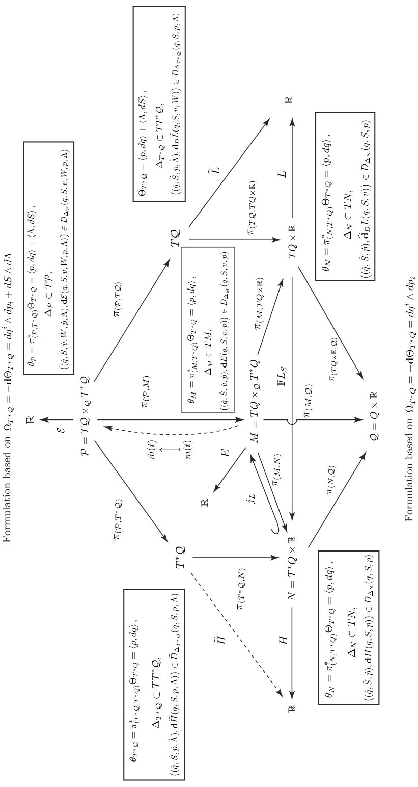 Figure 1
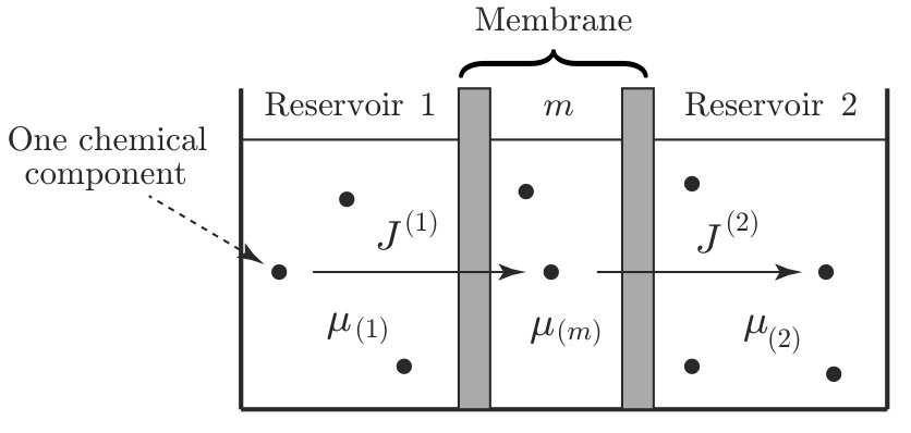 Figure 2
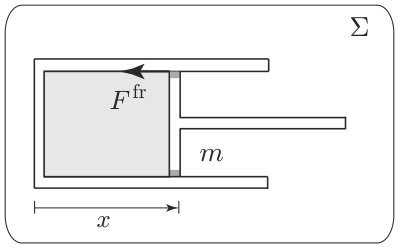 Figure 3
Peer Reviews
No public reviews on file for this paper yet. If you reviewed it on a platform where reviews are public (OpenReview, ICLR, NeurIPS, ICML), you can paste yours below so the community can read it here.
Videos
No videos yet. Explain this paper in a talk, walkthrough, or lecture? Add one.
Dirac structures in nonequilibrium thermodynamics
François Gay-Balmaz Hiroaki Yoshimura
CNRS, LMD, IPSL School of Science and Engineering
Ecole Normale Supérieure Waseda University
24 Rue Lhomond 75005 Paris, France Okubo, Shinjuku, Tokyo 169-8555, Japan
[email protected] [email protected]
Abstract
Dirac structures are geometric objects that generalize both Poisson structures and presymplectic structures on manifolds. They naturally appear in the formulation of constrained mechanical systems. In this paper, we show that the evolution equations for nonequilibrium thermodynamics admit an intrinsic formulation in terms of Dirac structures, both on the Lagrangian and the Hamiltonian settings. In absence of irreversible processes these Dirac structures reduce to canonical Dirac structures associated to canonical symplectic forms on phase spaces. Our geometric formulation of nonequilibrium thermodynamic thus consistently extends the geometric formulation of mechanics, to which it reduces in absence of irreversible processes. The Dirac structures are associated to the variational formulation of nonequilibrium thermodynamics developed in Gay-Balmaz and Yoshimura [2016a, b] and are induced from a nonlinear nonholonomic constraint given by the expression of the entropy production of the system.
Contents
-
2 A class of constraints of the thermodynamic type and its Dirac formulations
-
2.1 Variational formulation for nonlinear nonholonomic systems
-
3 Dirac formulations induced from the thermodynamical symplectic form
-
4 Dirac formulations induced from the mechanical symplectic form
1 Introduction
Nonequilibrium thermodynamics is a phenomenological theory which aims to identify and describe the relations among the observed macroscopic properties of a physical system and to determine the macroscopic dynamics of this system with the help of fundamental laws (e.g. Stueckelberg and Scheurer [1974]). The field of nonequilibrium thermodynamics naturally includes macroscopic disciplines such as classical mechanics, fluid dynamics, elasticity, and electromagnetism. The main feature of nonequilibrium thermodynamics is the occurrence of the various irreversible processes, such as friction, mass transfer, and chemical reactions, which are responsible of entropy production.
It is well known that in absence of irreversible processes, the equations of motion of classical mechanics, i.e., the Euler-Lagrange equations, can be derived from Hamilton’s variational principle applied to the action functional associated to the Lagrangian of the mechanical system. This variational formulation is intimately related to the existence of fundamental geometric structures in mechanics such as the canonical symplectic form on phase space, relative to which the equations of motion can be written in Hamiltonian form. It has been a challenging question to systematically extend both the variational and the geometric structures from the setting of classical mechanics to that of nonequilibrium thermodynamics.
In Gay-Balmaz and Yoshimura [2016a, b], we proposed an answer to the question regarding the variational structures by presenting a variational formulation for nonequilibrium thermodynamics which extends Hamilton’s principle of classical mechanics to include irreversible processes. This approach was developed for discrete and continuum systems with various irreversible processes such as heat transfer, matter transfer, viscosity, and chemical reactions. The variational formulation involves two types of constraints: a phenomenological constraint that needs to be satisfied by the critical curve of the action functional; and a variational constraint that imposes conditions on the variations of the curve to be considered.
In this paper, we shall show that Dirac structures provide appropriate geometric objects underlying nonequilibrium thermodynamics. These structures are associated to the variational formulation developed in Gay-Balmaz and Yoshimura [2016a, b].
Dirac structures are geometric objects that generalize both (almost) Poisson structures and (pre)symplectic structures on manifolds. They were originally developed by Courant and Weinstein [1988], Courant [1990], and Dorfman [1993], who also considered the associated constrained dynamical systems. Dirac structures were named after Dirac’s theory of constraints, see, Dirac [1950]. It was shown that Dirac structures are appropriate geometric objects for the formulation of electric circuits, van der Schaft and Maschke [1995a]; Bloch and Crouch [1997], and nonholonomic mechanical systems, van der Schaft and Maschke [1995b], in the context of implicit Hamiltonian systems, which yield implicit differential-algebraic equations as the evolution equations. It was further shown in Yoshimura and Marsden [2006a, b] that, in the Lagrangian setting, the Lagrange-d’Alembert equations of nonholonomic mechanics and its associated variational structure, can be formulated in terms of Dirac structures, as implicit Lagrangian systems.
The geometry of equilibrium thermodynamics has been mainly studied via contact geometry, following the initial works of Gibbs [1873a, b] and Carathéodory [1909], by Hermann [1973] and further developments by Mrugala [1978, 1980], Mrugala, Nulton, Schon, and Salamon [1991]. The contact manifold in this setting is called the thermodynamic phase space with contact form given by the Gibbs form, typically, where denotes the energy and are pairs of conjugated extensive and intensive variables. In this geometric setting, thermodynamic properties are encoded by Legendre submanifolds of the thermodynamic phase space. A step towards a geometric formulation of irreversible processes was made in Eberard, Maschke, and van der Schaft [2007] by lifting port Hamiltonian systems to the thermodynamic phase space. The underlying geometric structure in this construction is again a contact form.
As mentioned above, in this paper we shall show that the equations of motion for nonequilibrium thermodynamics can be formulated in the context of Dirac structures that are associated with the Lagrangian variational setting developed in Gay-Balmaz and Yoshimura [2016a, b]. More precisely, we shall prove that the equations of motion can be naturally formulated as Dirac dynamical systems based either on the generalized energy, the Lagrangian, or the Hamiltonian. To do this, we will extend the use of Dirac structures from the case of linear nonholonomic constraints to a class of nonlinear nonholonomic constraints which we will call of the thermodynamic type. In the case of nonequilibrium thermodynamics, the nonlinear constraint is given by the expression of entropy production associated to the irreversible processes involved in the system.
Variational formulation for nonequilibrium thermodynamics of simple systems.
A discrete thermodynamic system is a collection of a finite number of interacting simple systems . By definition, a simple thermodynamic system111In Stueckelberg and Scheurer [1974] they are called élément de système (French). We choose to use the English terminology simple system instead of system element. is a macroscopic system for which one (scalar) thermal variable and a finite set of mechanical variables are sufficient to describe entirely the state of the system. From the second law of thermodynamics, we can always choose the thermal variable as the entropy , see Stueckelberg and Scheurer [1974]. A system is said to be adiabatically closed if there is no exchange of matter and heat with the exterior of the system. It is said to be isolated if, in addition, there is no exchange of mechanical work with the exterior of the system.
We now quickly review from Gay-Balmaz and Yoshimura [2016a] the variational formulation of nonequilibrium thermodynamics in the particular case of simple adiabatically closed systems, which are the focus of the present paper. Let be the configuration manifold associated to the mechanical variables of the system, assumed to be of finite dimensions. The Lagrangian is a function , where denotes the tangent bundle of . We assume that the system involves exterior and friction forces which are fiber preserving maps .
A curve , is a solution of the variational formulation of nonequilibrium thermodynamics if it satisfies the variational condition
[TABLE]
for all variations and subject to the constraint
[TABLE]
with , and if it satisfies the nonlinear nonholonomic constraint
[TABLE]
From this variational formulation, we deduce the equations of motion for the adiabatically closed simple system as
[TABLE]
The variational formulation (1.1)–(1.3) is an extension of the Hamilton principle of mechanics to the case of nonequilibrium thermodynamics. In absence of the entropy variable , this variational formulation recovers the Hamilton principle and (1.4) reduces to the Euler-Lagrange equations with external force.
Note that the explicit expression of the constraint (1.3) involves phenomenological laws for the friction force , this is why we refer to it as a phenomenological constraint. The associated constraint (1.2) is called a variational constraint since it is a condition on the variations to be used in (1.1). The constraint (1.3) is nonlinear and one passes from the variational constraint to the phenomenological constraint by formally replacing the variations , , by the time derivatives , . Such a simple correspondence between the phenomenological and variational constraints still holds for the more general thermodynamic systems considered in Gay-Balmaz and Yoshimura [2016a, b].
If the simple system is not adiabatically closed, then the phenomenological constraint (1.3) becomes
[TABLE]
where denotes the external heat power supply, see Gay-Balmaz and Yoshimura [2016a].
In the present paper we shall focus on the case of simple isolated systems, i.e., adiabatically closed simple systems in which . The case can be easily included in the Dirac formulation, see Remark 4.6. From now on, we shall refer to these systems as simple systems.
Since the partial derivative of the Lagrangian is interpreted as minus the temperature of the system, we shall always assume
[TABLE]
It should be noted that the system (1.4) (with the external power included as in (1.5)) is the general form of the evolution equation for all simple systems, i.e., systems in which one scalar thermal variable is sufficient, in addition to configurational variables, to describe entirely the system. The system (1.4) also covers the case of simple systems arising in chemical reactions and electric circuits, see Gay-Balmaz and Yoshimura [2016a] and §5. The variational formulation (1.1)–(1.3) has been extended to general discrete systems in Gay-Balmaz and Yoshimura [2016a] which involve internal mass and heat transfer, as well as to continuum systems such as multicomponent viscous heat conducting fluid with chemical reactions in Gay-Balmaz and Yoshimura [2016b], and atmospheric thermodynamics in Gay-Balmaz [2017]. We refer to Gay-Balmaz and Yoshimura [2017b] for a variational formulation based on the free energy. For non simple systems, the variational approach is based on the concept of thermodynamic displacement.
Remark 1.1** (Inclusion of linear nonholonomic mechanical constraints).**
Linear nonholonomic mechanical constraints can be naturally included in this variational formulation. Suppose that the mechanical motion is constrained by a regular distribution (i.e., a smooth vector subbundle) . The variational formalism (1.1)–(1.3) is modified by considering, in addition to the variational constraint (1.2), the variational constraint and, in addition to the phenomenological constraint (1.3), the nonholonomic constraint . This is a thermodynamic extension of the Lagrange-d’Alembert principle used in nonholonomic mechanics, see, e.g., Bloch [2003]. **
Example.
A typical example of a simple thermodynamic system is the case of a perfect gas confined by a piston in a cylinder as illustrated in Fig. 1.1. In this case the configuration space of the mechanical variable is and the Lagrangian is given by , where is the mass of the piston, 222The state functions for a perfect gas are and , where is a constant depending exclusively on the gas (e.g. for monoatomic gas, for diatomic gas) and is the universal gas constant. From this, it is deduced that the internal energy reads
is the internal energy of the gas, is the number of moles, is the volume, and is the area of the cylinder with constant value. The friction force reads , where is the phenomenological coefficient, determined experimentally. From (1.4), we immediately get the coupled mechanical and thermal evolution equations for this system as
[TABLE]
where is the pressure and is the temperature. We refer to Gruber [1999] for a derivation of the equations of motion for this system by following the systematic approach of Stueckelberg and Scheurer [1974].
Plan of the paper.
In §2, we consider a special class of implicit second order differential-algebraic equations with nonlinear constraints arising from the Lagrange-d’Alembert principle. We refer to the constraints in this class as ”constraints of the thermodynamic type”. We show that these equations admit two types of Dirac formulations, one based on the generalized energy, the other one on the Lagrangian. The Dirac structure for the first case is defined on the Pontryagin bundle (the direct sum of the velocity and phase spaces) while the Dirac structure for the second case is defined on the phase space (cotangent bundle). In §3, we make use of these results to develop two Dirac formulations for the thermodynamics of simple systems. Associated to the first Dirac formulation there exists a variational formulation, the Lagrange-d’Alembert-Pontryagin principle, compatible with the variational formulation for simple systems given in Gay-Balmaz and Yoshimura [2016a]. The Dirac structures constructed in this case are induced by the canonical symplectic form on the thermodynamic configuration space. In §4, we develop Dirac formulations, with Dirac structures induced from the canonical symplectic form on the mechanical configuration space. These Dirac formulations can be written in terms of the generalized energy, the Lagrangian, or the Hamiltonian. We also explain the relation between the different Dirac formulations obtained. Finally, in §5 we illustrate the Dirac formulations with examples of simple thermodynamic systems involving irreversible processes associated to friction, mass transfer, and chemical reactions.
We finish this introduction by recalling below the definition of Dirac structures on manifolds and the associated Dirac dynamical systems. We also comment on the role of two canonical symplectic forms: one is associated to the mechanical configuration space and the other to the thermodynamic configuration space.
Dirac structures, Dirac dynamical systems, and nonholonomic mechanics.
Let be a manifold and consider the Pontryagin vector bundle over endowed with the symmetric fiberwise bilinear form
[TABLE]
for . A Dirac structure on (also called an almost Dirac structure) is by definition a vector subbundle , such that relative to , see Courant [1990].
For example, given a two-form and a distribution on (i.e., a vector subbundle of ), the subbundle defined by, for each ,
[TABLE]
is a Dirac structure on . In this paper, we shall extensively use this construction of Dirac structure.
Given a Dirac structure on and a function , the associated Dirac dynamical system for a curve is
[TABLE]
Note that in general (1.9) is a system of implicit differential-algebraic equations and the questions of existence, uniqueness or extension of solutions for a given initial condition can present several difficulties.
The formulation (1.9) offers a unified treatment for the equations of nonholonomic mechanics with (possibly degenerate) Lagrangian. Let us quickly recall how this proceeds. Consider a mechanical system with configuration manifold , a Lagrangian and a constraint distribution . Let be the Pontryagin bundle of and define the induced distribution , where is the projection defined by . We consider the Dirac structure induced, via (1.8), by the distribution and the presymplectic form on , where is the canonical symplectic form on and is the projection defined by . Then, the equations of motion for the nonholonomic system can be written in the form of the Dirac dynamical system on the Pontryagin bundle as
[TABLE]
where , defined by is the generalized energy associated to . System (1.10) is equivalent to the implicit differential-algebraic equation
[TABLE]
where denotes the annihilator of in . This system implies the Lagrange-d’Alembert equations
[TABLE]
for the nonholonomic system, see Yoshimura and Marsden [2006b].
There is an alternative Dirac formulation of the implicit system (1.11) that makes use of the Dirac structure on (instead of ) associated to the canonical symplectic form on and to the distribution induced on by . This formulation is directly based on the Lagrangian function and reads
[TABLE]
where is the Dirac differential whose definition will be reviewed later. The system (1.12) is called the Lagrange-Dirac system.
In the hyperregular case, the equations can be also written in terms of the Hamiltonian in the Hamilton-Dirac form
[TABLE]
In the present paper we shall show that the equations of evolution for the thermodynamics of simple systems can be written in the Dirac dynamical system form (1.10) and in the Lagrange-Dirac form (1.12) in two ways, as well as in the Hamilton-Dirac form (1.13), see Fig. 4.1. In the case of thermodynamics, however, one starts with a nonlinear constraint. We shall restrict our discussion to the case of simple thermodynamic systems and leave the development of the corresponding Dirac approach to general thermodynamic systems for a future work.
Mechanical and thermodynamic configuration spaces.
As mentioned earlier, in absence of the entropy variable, both constraints disappear and the variational formulation (1.1)–(1.3) recovers Hamilton’s principle of classical mechanics. In this case the intrinsic geometric structure is usually given by the canonical symplectic form on the cotangent bundle of the configuration manifold of the mechanical system, locally given as
[TABLE]
It is therefore expected that when thermodynamics is included, the relevant geometric structure should be naturally induced from this canonical structure. We shall show in this paper that this is indeed the case, namely, the appropriate Dirac structures are induced by the canonical symplectic form and by a distribution built from the phenomenological constraint. These Dirac structures are developed on and for the generalized energy and the Lagrangian formulations, respectively.
In addition, we will see that the canonical symplectic structure on the thermodynamic configuration space
[TABLE]
locally given by
[TABLE]
can be also used as the fundamental intrinsic form from which Dirac structures are deduced.
2 A class of constraints of the thermodynamic type and its Dirac formulations
In this section, we first recall a generalized Lagrange-d’Alembert principle for nonlinear nonholonomic mechanics, which involves two types of constraints, the kinematic and variational constraints. Then we focus on a specific situation, relevant with thermodynamics, for which the kinematic constraint is deduced from the variational constraint. We show that in this specific case, which we call “constraints of the thermodynamic type”, the equations of motion derived from the Lagrange-d’Alembert principle admit two types of Dirac formulations; one associated to a Dirac structure on the cotangent bundle and the other one associated to a Dirac structure on the Pontryagin bundle.
2.1 Variational formulation for nonlinear nonholonomic systems
The Lagrange-d’Alembert principle.
Consider a configuration manifold and a Lagrangian function defined on the tangent bundle of the configuration manifold. The general formulation of the Lagrange-d’Alembert principle, considered in Cendra, Ibort, de León, and Martín de Diego [2004], involves the choice of two distinct constraints, the kinematical and variational constraints, which, following Marle [1998] must in general be considered as independent notions. The kinematical constraint is given by a submanifold and describes a restriction on the motion of the mechanical system. The variational constraint is a subset such that for all the sets
[TABLE]
are vector spaces, the spaces of virtual displacements.
For simplicity, we assume that , where is the tangent bundle projection, we assume that is a submanifold and also that all the vector spaces have the same (strictly positive) dimension. These hypotheses are not needed to apply the Lagrange-d’Alembert principle, however, since they are verified in the case of interest for this paper, we shall assume them. We also refer to Cendra and Grillo [2007] for a general treatment of the constraint sets and .
By definition, a curve is a solution of the Lagrange-d’Alembert principle for if and
[TABLE]
for all variations of the curve with fixed endpoints, such that
[TABLE]
By applying this principle, one obtains that a curve is a solution of the Lagrange-d’Alembert principle for if and only if it satisfies the following implicit second order differential-algebraic equations
[TABLE]
We shall not discuss here the question of the existence and uniqueness of solutions of this implicit differential equation since in our case of interest for thermodynamics, see §3, it reduces to an explicit differential equation.
Nonlinear constraints of the thermodynamic type.
We now present a setting that is well adapted for the description of the nonequilibrium thermodynamics of simple systems. From now on, we shall denote the configuration manifold by , while we use the notation exclusively for the configuration manifold associated to the mechanical variables. As we will see in §3 when applying this setting to thermodynamics, the configuration manifold contains mechanical variables as well as thermodynamic variables, so it is referred to as the thermodynamic configuration space.
In the setting that we now develop, the variational constraint is chosen first and the kinematic constraint is defined from it as follows:
[TABLE]
Thus, if is locally given by equations , then is locally given by .
Note that in this setting, it is the variational constraint which determines the kinematic constraint, and not the converse as in the Chetaev case. Note also that in general is a nonlinear nonholonomic constraint.
In the case of a kinematic constraint given by (2.2), the implicit second order differential-algebraic equation (2.1) becomes
[TABLE]
where we note that is equivalent with . One directly computes that the energy , defined by
[TABLE]
is constant along the solutions of the system (2.3), for any choice of variational constraint .
We shall present two Dirac formulations for the implicit second order differential equations (2.1). These two formulations, on the Pontryagin bundle and on the cotangent bundle , extend the corresponding Dirac formulations (1.10) and (1.12) of nonholonomic mechanics, respectively. While the first formulation uses the generalized energy and its ordinary differential, the second formulation uses the Lagrangian and its Dirac differential.
2.2 Dirac formulation on the Pontryagin bundle
In this section we develop the Dirac dynamical system formulation on the Pontryagin bundle for systems with nonlinear nonholonomic constraints of the thermodynamic type. The Dirac structure is defined from the presymplectic form on induced by the canonical symplectic form on and from a distribution on induced by the given variational constraint . This results in a Dirac dynamical system extending (1.10) to the case of nonlinear constraints of the thermodynamic type.
Induced Dirac structure.
From a given variational constraint , we construct the induced distribution on the Pontryagin bundle , defined by:
[TABLE]
Locally, the distribution reads
[TABLE]
Consider the presymplectic form on induced from the canonical symplectic form on by the projection . To the distribution and the presymplectic form is naturally associated the induced Dirac structure on defined as
[TABLE]
where we used the notation . Note that this definition follows the construction of a Dirac structure recalled in (1.8), with , and . Locally, one directly checks that \big{(}(q,v,p,\dot{q},\dot{v},\dot{p}),(q,v,p,\alpha,\beta,u)\big{)}\in D_{\Delta_{\mathcal{P}}}(q,v,p) is equivalent to
[TABLE]
Dirac dynamical system formulation on .
Given a Lagrangian function , we define the generalized energy on the Pontryagin bundle as
[TABLE]
Using the local expression \mathbf{d}\mathcal{E}(q,v,p)=\big{(}q,v,p,-\frac{\partial L}{\partial q},p-\frac{\partial L}{\partial v},v\big{)} for the differential of together with (2.6), it follows that \big{(}(q,v,p,\dot{q},\dot{v},\dot{p}),\mathbf{d}\mathcal{E}(q,v,p)\big{)}\in D_{\widetilde{C}_{V}}(q,v,p) is equivalent to
[TABLE]
One observes that from the definition of given in (2.2) and from the third equation, the first equation is equivalent to . This is a key step that explicitly involves the fact that the kinematic constraint is determined from the variational constraint via the definition (2.2). Therefore, we get from (2.8) the implicit form of the equations (2.3) associated to the constraints of the thermodynamic type. These results are summarized in the following Theorem.
Theorem 2.1**.**
Consider a variational constraint , the associated kinematic constraint of the thermodynamic type defined in (2.2), and the associated Dirac structure on defined in (2.5). Let be a Lagrangian function and be the associated generalized energy. Then the following statements are equivalent:
- •
The curve satisfies the implicit first order differential-algebraic equations
[TABLE]
- •
The curve satisfies the Dirac dynamical system
[TABLE]
Moreover, the system (2.9) is equivalent to the implicit second order differential-algebraic equations on given by
[TABLE]
associated to constraints of the thermodynamic type.
The Lagrange-d’Alembert-Pontryagin principle.
We now show that the evolution equations (2.9) associated to the Dirac dynamical system on the Pontryagin bundle have a natural variational structure, called the Lagrange-d’Alembert-Pontryagin principle. This is similar to the situation of Dirac dynamical systems in linear nonholonomic mechanics, see Yoshimura and Marsden [2006b], which also admit such variational structures.
For constraints of the thermodynamic type, the Lagrange-d’Alembert-Pontryagin principle for a curve in the Pontryagin bundle reads as follows:
[TABLE]
for variations such that and , and where the curve satisfies . In terms of , these conditions intrinsically read , , and . Notice that the variational formulation (2.10) may be restated in terms of the generalized energy , see (2.7), as
[TABLE]
with respect to the same class of variations as before. One checks that a curve satisfies the principle (2.10) if and only if it is a solution of the equations (2.9), thus called the Lagrange-d’Alembert-Pontryagin equations associated to and .
This variational formulation can be intrinsically given as follows. Consider the one-form , where is the canonical one-form on . In coordinates, we have . With the help of this one-form, the principle (2.11) can be written as
[TABLE]
with respect to the same class of variations as before. This yields the intrinsic Lagrange-d’Alembert-Pontryagin equations:
[TABLE]
where is the presymplectic form on considered earlier.
2.3 Lagrange-Dirac formulation
In this section we develop the Lagrange-Dirac formulation for systems with nonlinear nonholonomic constraints of the thermodynamic type. We define the Dirac structure on from the canonical symplectic form on and from a distribution on induced by the given variational constraint . This results in a Lagrange-Dirac system extending (1.12) to the case of nonlinear constraints of the thermodynamic type.
Induced Dirac structure.
From a given variational constraint and a given Lagrangian , we assume that it is possible to define the variational constraint by
[TABLE]
where is such that . The assumption under this definition is that the right hand side of (2.12) does not depend on the choice of such that holds. This assumption holds for instance when is nondegenerate. However, in §3, we will show that this construction can be used even for a special case in which is degenerate.
Using the cotangent bundle projection we construct from the induced distribution on as
[TABLE]
Locally, the distribution reads
[TABLE]
To the distribution and the canonical symplectic form on is naturally associated the induced Dirac structure on defined, for , by
[TABLE]
Locally, one directly checks that \big{(}(q,p,\dot{q},\dot{p}),(q,p,\alpha,u)\big{)}\in D_{\Delta_{T^{*}\mathcal{Q}}}(q,p) is equivalent to
[TABLE]
Lagrange-Dirac formulation on .
Given a Lagrangian function , the Dirac differential of the Lagrangian is the map defined by
[TABLE]
where is the canonical diffeomorphism, locally given by , see, Yoshimura and Marsden [2006a]. Using the local expression (2.15), one checks that \big{(}(q,p,\dot{q},\dot{p}),\mathbf{d}_{D}L(q,v)\big{)}\in D_{\Delta_{T^{*}\mathcal{Q}}}(q,p) is equivalent to
[TABLE]
We thus get again the implicit form of the equations (2.3) associated to the nonholonomic constraints of the thermodynamic type. These results are summarized in the following Theorem.
Theorem 2.2**.**
Consider a variational constraint and the associated kinematic constraint of the thermodynamic type defined in (2.2). Let be a Lagrangian function, be the variational constraint as in (2.12), and define the induced Dirac structure as in (2.14). Then the following statements are equivalent:
- •
The curve satisfies the implicit first order differential-algebraic equations
[TABLE]
- •
The curve satisfies the Lagrange-Dirac system
[TABLE]
Moreover, the system (2.16) is equivalent to the implicit second order differential-algebraic equations on given by
[TABLE]
associated to nonlinear nonholonomic constraints of the thermodynamic type.
Remark 2.3** (The special case of mechanical systems with linear nonholonomic constraints).**
In the particular case of linear nonholonomic constraints in mechanics, the previous two Dirac formulations recover those of nonholonomic mechanical systems developed in Yoshimura and Marsden [2006a]. In this case and we assume that a Lagrangian and a distribution are given. The kinematic and variational constraints are given by and (so that ) and the Lagrange-d’Alembert equations (2.17) become
[TABLE]
For the case of the Dirac dynamical system formulation on studied in §2.2, the induced distribution defined in (2.4) is which recovers the distribution used in (1.10). For the case of the Lagrange-Dirac formulation on studied in the present section, the hypothesis underlying the definition (2.12) is clearly verified for any Lagrangian (whether is degenerate or not). We can thus define and from (2.13), we have , which recovers the distribution used in (1.12).
In conclusion, in the special case , , and , the Dirac formulations of Theorem 2.1 and Theorem 2.2 recover the corresponding Dirac formulations for nonholonomic mechanics (1.10) and (1.12).**
3 Dirac formulations induced from the thermodynamical symplectic form
In this section, we first show that the equations of evolution for the thermodynamics of simple systems fall into the class that is considered in §2. Then, by applying the results of §2, we obtain the corresponding Dirac formulations for the thermodynamics of such systems, namely, a Dirac dynamical system formulation on the Pontryagin bundle and a Lagrange-Dirac formulation. We also present the associated Lagrange-d’Alembert-Pontryagin variational structures.
3.1 Dirac formulation on the Pontryagin bundle
Constraints for the thermodynamics of simple systems.
Let us consider a simple thermodynamic system with a Lagrangian and a friction force . For simplicity, we assume that , see Remark 4.6. Here is the configuration manifold of the mechanical variables of the system, and denotes the space of the thermodynamic variable. Let us further introduce the thermodynamic configuration manifold . Then, the variational constraint (1.2) defines the subset
[TABLE]
where , , and . Since by hypothesis, see (1.6), we obtain that is a submanifold of of codimension one.
The kinematic constraint defined from the variational constraint in (2.2) is given here by
[TABLE]
which hence coincides with the phenomenological constraint (1.3). This justifies the terminology “constraint of the thermodynamic type” used for the general setting developed in §2 which naturally includes the types of constraints arising in thermodynamics.
For each fixed , the annihilator of is given by
[TABLE]
By using the expression of (3.2) and (3.3), and the fact that the Lagrangian does not depend on , the system (2.1) yields
[TABLE]
This recovers the equations of motion for the thermodynamics of a simple system, which is recalled in (1.4) with .
Let be the Pontryagin bundle over . Using the notation for an element of the Pontryagin bundle , the distribution induced by on , defined in (2.4) with the help of the projection , as , reads locally
[TABLE]
Dirac dynamical system formulation on .
As in (2.5), we define the Dirac structure on induced from the distribution and the presymlectic form on as
[TABLE]
Writing locally and , where , and , the induced Dirac structure on is locally described as follows: \big{(}(x,\dot{x}),(x,\zeta)\big{)}\in D_{\Delta_{\mathcal{P}}}(x) is equivalent to
[TABLE]
The generalized energy defined in (2.7) is given here by
[TABLE]
Using the expression \mathbf{d}\mathcal{E}(q,S,v,W,p,\Lambda)=\big{(}q,S,v,W,p,\Lambda,-\frac{\partial L}{\partial q},-\frac{\partial L}{\partial S},p-\frac{\partial L}{\partial v},\Lambda,v,W\big{)}, the Dirac dynamical system \big{(}(x,\dot{x}),\mathbf{d}\mathcal{E}(x)\big{)}\in D_{\Delta_{\mathcal{P}}}(x), for , yields
[TABLE]
We thus obtain the following theorem concerning the Dirac formulation of the thermodynamics of simple systems.
Theorem 3.1**.**
Consider a simple system with a Lagrangian and a friction force . Then the following statements are equivalent:
- •
The curve x(t):=\big{(}q(t),S(t),v(t),W(t),p(t),\Lambda(t)\big{)}\in\mathcal{P} satisfies the equations
[TABLE]
- •
The curve satisfies the Dirac dynamical system
[TABLE]
Moreover, the system (3.6) is the implicit version of the system of evolution equations
[TABLE]
for the thermodynamics of simple systems.
Proof. The result follows from Theorem 2.1 and the expressions (3.1)–(3.4) computed above. It also follows from the expression of the generalized energy , given in (3.5) and the expression of its differential .
The Lagrange-d’Alembert-Pontryagin principle on .
As explained in §2.2, to any Dirac dynamical system on the Pontryagin bundle with constraints of thermodynamic type, is naturally associated a variational formulation on the Pontryagin bundle, called the Lagrange-d’Alembert-Pontryagin principle. We now describe this variational formulation for the case of the thermodynamics of adiabatically closed simple systems.
For a curve x(t)=\big{(}q(t),S(t),v(t),W(t),p(t),\Lambda(t)\big{)}\in\mathcal{P}, the Lagrange-d’Alembert-Pontryagin principle on given in (2.10) becomes here
[TABLE]
for variations \delta x(t)=\big{(}\delta q(t),\delta S(t),\delta v(t),\delta W(t),\delta p(t),\delta\Lambda(t)\big{)} of the curve that satisfy
[TABLE]
and , and where the curve is subject to the phenomenological constraint
[TABLE]
From this principle, one derives the associated Lagrange-d’Alembert-Pontryagin equations given by
[TABLE]
which are manifestly equivalent with the evolution equations for the Dirac dynamical system obtained in (3.6).
Using the generalized energy , it follows that the variational formulation (3.9) can be rewritten as
[TABLE]
for the admissible variations that satisfy (3.10), where the curve satisfies the nonholonomic constraint (3.11). Note that this principle is a Hamilton-Pontryagin version of the variational formulation developed in Gay-Balmaz and Yoshimura [2016a].
The intrinsic Lagrange-d’Alembert-Pontryagin equations for thermodynamics.
The variational formulation can be intrinsically written as follows. Consider the projection , and the one-form , where is the canonical one-form on . In coordinates, we have . With the help of this one-form, the variational formulation (3.12)–(3.11) reads, for a curve ,
[TABLE]
with respect to variations such that and , and with the constraint . From this principle it follows the intrinsic Lagrange-d’Alembert-Pontryagin equations for thermodynamics as
[TABLE]
where is the presymplectic form considered earlier. In coordinates it reads . Equation (3.13) is the intrinsic formulation of the system (3.6).
3.2 Lagrange-Dirac formulation
In the above, we have presented the Dirac dynamical system formulation for the thermodynamics of simple systems, by using a Dirac structure on the Pontryagin bundle , following the developments of §2.2. In this section we show the Lagrange-Dirac formulation for such systems by using a Dirac structure on the cotangent bundle , following the developments of §2.3.
Constraints for the thermodynamics of simple systems.
Consider a Lagrangian and assume it is hyperregular with respect to the mechanical variables, i.e., the map
[TABLE]
is a diffeomorphism for each fixed , see Gay-Balmaz and Yoshimura [2017a] for more details. Under this hypothesis, following (2.12), given the variational constraint in (3.1), we can define the variational constraint as
[TABLE]
where is uniquely determined by the condition . Note that by using the projection , , we can lift the Lagrangian onto as . The lifted Lagrangian is not regular since it does not depend on . Nevertheless, for the case of thermodynamics, the variational constraint (3.15) is well-defined, because the right hand side does not depend on . This is a case where the definition (2.12) can still be used even though the Lagrangian (here ) is degenerate. Explicitly, we have
[TABLE]
where and , in which is uniquely determined from the condition .
Using the notation , the induced distribution on , defined in (2.13) with the help of the projection as
[TABLE]
reads locally
[TABLE]
Lagrange-Dirac formulation on .
Given the distribution and the canonical symplectic form , one can define the induced Dirac structure on by
[TABLE]
for each . Writing locally and , with , and , the condition \big{(}(z,\dot{z}),(z,\zeta)\big{)}\in D_{\Delta_{T^{*}\mathcal{Q}}}(z) is equivalent to
[TABLE]
From this local expression, it follows that
[TABLE]
if and only if
[TABLE]
where the last two equalities come from the fact that and both belong to fibers at the point . Recall that
[TABLE]
One thus obtains the following Lagrange-Dirac formulation for the thermodynamic of simple systems.
Theorem 3.2**.**
Consider a simple system with a Lagrangian and a friction force . Assume that is hyperregular with respect to the mechanical variables and define and as before. Then the following statements are equivalent:
- •
The curve \big{(}q(t),S(t),v(t),W(t),p(t),\Lambda(t)\big{)}\in\mathcal{P} satisfies the equations
[TABLE]
- •
The curve satisfies the Lagrange-Dirac system
[TABLE]
Moreover, the system (3.18) is an implicit version of the system of evolution equations (3.8) for the thermodynamics of simple systems.
4 Dirac formulations induced from the mechanical symplectic form
In this section, we show that Dirac formulations of nonequilibrium thermodynamics of simple systems can be constructed by using the canonical symplectic form on the cotangent bundle of the mechanical configuration manifold . In this case, we can develop a Hamilton-Dirac description.
4.1 Dirac formulation on
We consider the vector bundle on given by
[TABLE]
whose vector fiber at is . An element in this fiber is denoted as . Note that we can write as the pull-back of the Pontryagin bundle of , i.e., , where is the projection .
Constraints for the thermodynamics of simple systems.
In §3.1 we have considered the distribution on induced by the variational constraint in (3.1) associated to (1.2). We observe that the variational constraint does not depend on , so it can be used to yield a distribution on as
[TABLE]
It is locally given as
[TABLE]
Dirac formulation on .
Consider the projection
[TABLE]
and the presymplectic form on induced from the canonical symplectic form of . Denoting by an arbitrary element in , we define the Dirac structure on induced from the distribution and the presymlectic form as
[TABLE]
Writing locally and , where , and , the induced Dirac structure on is locally described as follows: for each , the condition \big{(}(m,\dot{m}),(m,\zeta)\big{)}\in D_{\Delta_{M}}(m) is equivalent to
[TABLE]
The generalized energy is defined here by
[TABLE]
Using the expression \mathbf{d}E(q,S,v,p)=\Big{(}q,S,v,p,-\frac{\partial L}{\partial q},-\frac{\partial L}{\partial S},p-\frac{\partial L}{\partial v},v\Big{)}, the Dirac dynamical system \big{(}(m,\dot{m}),\mathbf{d}E(m)\big{)}\in D_{\Delta_{M}}(m), for , yields
[TABLE]
We thus obtain the following theorem concerning the Dirac formulation of the thermodynamics of simple systems on .
Theorem 4.1**.**
Consider a simple system with a Lagrangian and a friction force . Then the following statements are equivalent:
- •
The curve satisfies the equations
[TABLE]
- •
The curve satisfies the Dirac dynamical system
[TABLE]
Moreover, the system (4.1) is the implicit version of the system of evolution equations
[TABLE]
for the thermodynamics of simple systems.
Lagrange-d’Alembert-Pontryagin principle on .
Let us now describe the variational formulation associated to the above Dirac dynamical system. Given a curve , we consider the Lagrange-d’Alembert-Pontryagin principle on given by
[TABLE]
for variations of the curve that satisfy
[TABLE]
and , and where the curve is subject to the phenomenological constraint
[TABLE]
It is easily verified that this principle yields the implicit system (4.1) on .
Intrinsic Lagrange-d’Alembert-Pontryagin equations on .
The above variational formulation can be intrinsically written as follows. Consider the projection , and the one-form , where is the canonical one-form on . In coordinates, we have . With the help of this one-form, the variational formulation (4.3)–(4.5) reads, for a curve ,
[TABLE]
with respect to variations of the curve such that and , and with the constraint . From this principle it follows the intrinsic Lagrange-d’Alembert-Pontryagin equations for thermodynamics on as
[TABLE]
where is the presymplectic form considered above. Equation (4.6) is the intrinsic formulation of the system (4.1).
4.2 Lagrange-Dirac formulation on
We describe here a Lagrange-Dirac formulation on associated to the Dirac structure on induced from the variational constraint and the canonical symplectic form on .
Constraints.
Consider a Lagrangian of a simple thermodynamic system and assume it is hyperregular with respect to the mechanical variables , see (3.14). Recall that in this case we can define from the constraint , see (3.15). Since does not depend on it induces the following distribution on :
[TABLE]
locally given as
[TABLE]
We recall the definition , in which is uniquely defined from the condition . Associated to this distribution and to the presymplectic form , is the Dirac structure on given by, for each ,
[TABLE]
Writing locally and , where , and , the induced Dirac structure on is locally described as follows: for each , the condition \big{(}(n,\dot{n}),(n,\zeta)\big{)}\in D_{\Delta_{N}}(n) is equivalent to
[TABLE]
Lagrange-Dirac formulation on .
Recall that the Dirac differential for a Lagrangian is defined by using the canonical diffeomorphism , locally given by . In our case, we extend to the diffeomorphism
[TABLE]
which is operating on as . Note that is a symplectic diffeomorphism with respect to the canonical symplectic structures and , where
[TABLE]
The associated Dirac differential of is
[TABLE]
From this definition and the expression (4.7) of the Dirac structure, we have
[TABLE]
if and only if
[TABLE]
where the last equality comes from the fact that and both belong to the fibers at . One thus obtains the following Lagrange-Dirac formulation for the thermodynamic of simple systems, based on the canonical symplecic form .
Theorem 4.2**.**
Consider a simple system with a Lagrangian and a friction force . Assume that is hyperregular with respect to the mechanical variables and define and as before. Then the following statements are equivalent:
- •
The curve satisfies the equations
[TABLE]
- •
The curve satisfies the Lagrange-Dirac system
[TABLE]
Moreover, the system (4.8) is an implicit version of the system of evolution equations (3.8) for the thermodynamics of simple systems.
4.3 Hamilton-Dirac formulation on
We assume that is hyperregular with respect to the mechanical variables, see (3.14). Under this assumption, we can define the Hamiltonian function by
[TABLE]
where is uniquely determined from by the condition .
We shall use the same distribution and the same Dirac structure as in §4.2 before. Note that in (4.7) we can directly write the constraint in terms of the Hamiltonian as . From (4.7), it follows that the Hamilton-Dirac system
[TABLE]
is equivalent to
[TABLE]
We get the following theorem.
Theorem 4.3**.**
Consider a simple system with a Lagrangian and a friction force . Assume that the Lagrangian is hyperregular with respect to the mechanical variables, consider the associated Hamiltonian and define as before. Then the following statements are equivalent:
- •
The curve satisfies the equations
[TABLE]
- •
The curve satisfies the Hamilton-Dirac system
[TABLE]
Moreover the system (4.11), equivalently written as
[TABLE]
is the Hamiltonian description of the system of evolution equations (3.8) for the thermodynamics of simple systems.
Hamilton-d’Alembert principle on .
To the Hamilton-Dirac formulation is naturally associated a variational structure. In our case, the variational formulation on is
[TABLE]
for all variations for the curve that satisfy
[TABLE]
with , and the curve is subject to the phenomenological constraint
[TABLE]
We refer to the principle (4.14)–(4.16) as the Hamilton-d’Alembert principle. From this principle one immediately obtains the system (4.13).
Intrinsic form of the Hamilton-d’Alembert principle on .
The variational formulation can be intrinsically written as follows. Let us define , where we recall that , and is the canonical one-form on .
The variational formulation is intrinsically described in terms of a curve as
[TABLE]
for all variations such that and , and with the constraint . It yields the following intrinsic Hamilton-d’Alembert equation on
[TABLE]
where . Equation (4.17) is the intrinsic expression of the system (4.13).
Remark 4.4** (Recovering the canonical formulation of classical mechanics).**
When does not depend on and the friction force is absent, it goes without saying that (4.17) reduces to the canonical symplectic formulation of Hamiltonian mechanics, namely,
[TABLE]
Relation between the Dirac formulations on and .
The Hamilton-Dirac formulation on presented in this section, namely
[TABLE]
is related, via the partial Legendre transform, to the Dirac formulation on presented in §4.1 given by
[TABLE]
Indeed, the partial Legendre transform induces the fiber preserving immersion
[TABLE]
over , where the function is defined by such that the condition holds.
One notices the following relations:
[TABLE]
[TABLE]
By using the explicit forms (4.1), resp., (4.13) of the systems (4.19), resp., (4.18) we notice that if the curve is a solution of the Hamilton-Dirac system (4.18), then the curve defined by is a solution of the Dirac dynamical system (4.19). Conversely, if the curve is a solution of the Dirac dynamical system (4.19), then the curve is of the form for a curve , because the relation is included in the system (4.19) (see the third equation in (3.6)). In addition, by inspection of the explicit forms (4.1) and (4.13), the curve is solution of the Hamilton-Dirac system (4.18).
Relation between the Dirac formulations on and .
We note that if the curve is a solution of the Dirac dynamical system (4.2) on , then the lifted curve defined by
[TABLE]
is a solution of the Dirac dynamical system (3.7) on . See Fig. 4.1 for an illustration of this relation.
Remark 4.5** (On Hamilton-Dirac formulations).**
Note that we have two Lagrange-Dirac formulations: one on which uses the Lagrangian , see §4.2, and one on which uses the lifted Lagrangian , see §3.2. On the Hamilton-Dirac side, however, we only have shown one formulation, on , described in the present section. There is no natural corresponding Hamilton-Dirac formulation on , because, in thermodynamics, the lifted Lagrangian is always degenerate, since it does not depend on .
Despite this degeneracy, one can define a Hamiltonian on by lifting the Hamiltonian as follows
[TABLE]
In this case, one recovers the equation of evolution for the thermodynamic of simple systems as a Hamilton-Dirac system for on by using a Dirac structure induced from the presymplectic form (not the canonical symplectic form ). Namely, we define
[TABLE]
where is the distribution defined in (3.16). Note that the Dirac structure (4.20) is distinct from the Dirac structure defined in (3.17). The condition \big{(}(z,\dot{z}),(z,\zeta)\big{)}\in\widetilde{D}_{\Delta_{T^{*}\mathcal{Q}}}(z) is equivalent to
[TABLE]
Thus, the Hamilton-Dirac system
[TABLE]
does yield the system (4.10). **
Remark 4.6** (Inclusion of the external force).**
An external force can be easily included in all the Dirac formulations. To do this, we consider the lift of the external force onto the manifold on which the Dirac structure is defined. For example, for the Dirac formulation on developed in §3.1, we consider the projections and , locally given by , and define the lifted external force as the horizontal one-form given by
[TABLE]
with . This external force is included in the Dirac dynamical system (3.7) as follows
[TABLE]
One easily checks that it yields the evolution equations (1.4). The case of the other Dirac formulations is treated similarly. **
5 Examples
We illustrate the Dirac formulations with three examples of simple systems, involving three different irreversible processes: friction, matter transfer, and chemical reactions.
The one-cylinder problem.
This example has been already described in §1, see Fig. 1.1. The thermodynamic configuration space is . We shall illustrate the approach of §4.1. The bundle reads . The Dirac structure is given as follows. For each , we have
[TABLE]
The generalized energy is
[TABLE]
and one directly checks that the Dirac dynamical system (4.2) yields the evolution equations (1.7) for the piston. The other formulations can be carried out similarly, by using the expressions
[TABLE]
Diffusion through a homogeneous membrane.
We consider a system with diffusion due to (internal) matter transfer through a homogeneous membrane separating two reservoirs, as considered in Oster, Perelson, Katchalsky [1973, §2.2]. The equations of evolution where derived in Gay-Balmaz and Yoshimura [2016a, §3.4] from the variational formalism, to which we refer for more details on this example. We suppose that the system is simple (so it is described by a single entropy variable) and involves a single chemical component. We denote by the number of mole of this chemical component in the membrane and also by and the numbers of mole in the reservoirs and , as shown in Fig. 5.1.
(1) Variational formulation based on the chemical potential. The approach developed in Gay-Balmaz and Yoshimura [2016a] is based on the internal energy , expressed in terms of the entropy and number of moles. We shall here describe the system by using the thermodynamic potential expressed in terms of the entropy and the chemical potentials, namely, we define the thermodynamic potential
[TABLE]
were on the right hand side are defined from the conditions .
The Lagrangian in this representation is defined as
[TABLE]
where . Let us denote by the flux from the reservoir into the membrane and the flux from the membrane into the reservoir . The variational formulation can be expressed as
[TABLE]
where the curves and satisfy the nonlinear nonholonomic constraint
[TABLE]
and with respect to variations and subject to the constraint
[TABLE]
with . This variational principle, together with the observation and the phenomenological constraint yield the evolution equations
[TABLE]
(2) Dirac formulation. The thermodynamic configuration space is with . The bundle reads , with , . The Dirac structure is given as follows. For each , we have
[TABLE]
The generalized energy is
[TABLE]
and one directly checks that the Dirac dynamical system (4.2) yields the evolution equation (5.2) for membrane transport.
The generalized energy on to be used in the Dirac formulation (3.7) is
[TABLE]
(3) The Hamiltonian. We note that the Lagrangian defined in (5.1) is nondegenerate in the sense of (3.14). The associate Hamiltonian defined in (4.9) recovers the internal energy, namely,
[TABLE]
The Hamilton-Dirac system (4.12) yields the evolution equations (5.2).
Chemical reactions dynamics.
Consider a system of several chemical components undergoing chemical reactions. Let be the chemical components and the chemical reactions. We denote by the number of moles of the component . Chemical reactions may be represented by
[TABLE]
where and are forward and backward reactions associated to the reaction , and , are forward and backward stoichiometric coefficients for the component in the reaction . From this relation, the number of moles has to satisfy
[TABLE]
where , is the degree of advancement of reaction , and is the rate of the chemical reaction . The mass conservation during each reaction is given by
[TABLE]
where is the molecular weight of component . We shall denote by , the internal energy of the system. We assume that the volume stay constant .
The variational formulation for the nonequilibrium thermodynamics of this system was presented in Gay-Balmaz and Yoshimura [2016a, §3.3] and is based on the Lagrangian defined by
[TABLE]
where and on the right hand side is expressed in terms of by
[TABLE]
which results from (5.3). The expression of the entropy production involves friction forces of the general form , where the symmetric part of the matrix is positive.
The thermodynamic configuration space is . The bundle reads , with , , . The Dirac structure is given as follows. For each , we have
[TABLE]
The generalized energy is
[TABLE]
and one obtains from the Dirac dynamical system (4.2) the evolution equations for the chemical reactions, which coincide with those derived in Gay-Balmaz and Yoshimura [2016a, §3.3]. The generalized energy on to be used in the Dirac formulation (3.7)
[TABLE]
The Lagrangian (5.4) is degenerate hence the Hamiltonian cannot be defined.
One can alternatively describe chemical reaction dynamics by using a thermodynamic potential analogous to the one introduced for matter transfer above. This alternative formulation is based on the approach for chemical reactions described in Gay-Balmaz and Yoshimura [2016a, Def. 3.7], in which case the Lagrangian is regular and a Hamiltonian can be defined.
Conclusion.
In this paper we have shown that the equations of motion for nonequilibrium thermodynamics can be formulated in the context of Dirac structures that are associated with the Lagrangian variational setting developed in Gay-Balmaz and Yoshimura [2016a, b]. We have considered the thermodynamics of simple systems, i.e., systems for which one entropy variable is sufficient to describe the irreversibility. We have proved that the equations of motion can be naturally formulated as Dirac dynamical systems based on either the generalized energy, the Lagrangian, or the Hamiltonian. These formulations are associated to either the canonical symplectic form on the thermodynamic phase space (§3) or the canonical symplectic form on the mechanical phase space (§4). These formulations are compatible with the geometric formulation of classical mechanics given in terms of the canonical symplectic form, which is recovered in absence of the entropy variable and friction forces. We have explained the link between the various Dirac formulations and summarised it in Fig. 4.1. Finally we have illustrated these formulations with examples involving the irreversible processes of friction, matter transfer, and chemical reactions.
Acknowledgement.
F.G.B. is partially supported by the ANR project GEOMFLUID, ANR-14-CE23-0002-01; H.Y. is partially supported by JSPS Grant-in-Aid for Scientific Research (26400408, 16KT0024, 24224004), the MEXT “Top Global University Project” and Waseda University (SR 2017K-167).
The reference list from the paper itself. Each links out to its DOI / PubMed record.
- 1Bloch [2003] Bloch, A. M. [2003], Nonholonomic Mechanics and Control , volume 24 of Interdisciplinary Applied Mathematics , Springer-Verlag, New York. With the collaboration of J. Baillieul, P. Crouch and J. Marsden, and with scientific input from P. S. Krishnaprasad, R. M. Murray and D. Zenkov.
- 2Bloch and Crouch [1997] Bloch, A. M. and P. E. Crouch [1997], Representations of Dirac structures on vector spaces and nonlinear L–C circuits. In: Differential Geometry and Control (Boulder, CO, 1997) . Vol. 64. pp. 103–117. Amer. Math. Soc. Providence, RI.
- 3Carathéodory [1909] Carathéodory, C. [1909], Untersuchungen über die Grundlagen der Thermodynamik, Math. Ann. , 67 , 355–386.
- 4Cendra and Grillo [2007] Cendra, H. and S. D. Grillo [2007], Lagrangian systems with higher order constraints, J. Math. Phys. 48 052904.
- 5Cendra, Ibort, de León, and Martín de Diego [2004] Cendra, H., A. Ibort, M. de León, and D. de Diego [2004], A generalization of Chetaev’s principle for a class of higher order nonholonomic constraints, J. Math. Phys. 45 , 2785.
- 6Courant [1990] Courant, T. J. [1990], Dirac manifolds, Trans. Amer. Math. Soc. , 319 , 631–661.
- 7Courant and Weinstein [1988] Courant, T. and A. Weinstein [1988], Beyond Poisson structures. In: Action hamiltoniennes de groupes. Troisième théorème de Lie (Lyon, 1986) . Vol. 27. pp. 39–49. Hermann. Paris.
- 8Dirac [1950] Dirac, P. A. M. [1950], Generalized Hamiltonian dynamics, Canad. J. Math. , 2 , 129–148.