Optimal Threshold Design for Quanta Image Sensor
Omar A. Elgendy, Stanley H. Chan

TL;DR
This paper develops an optimal threshold design framework for Quanta Image Sensors, showing that spatially varying thresholds improve image quality and proposing a practical bisection-based update scheme.
Contribution
It introduces a theoretical oracle threshold matching pixel intensity and a practical asymptotically unbiased threshold update method.
Findings
Improved convergence rate over existing methods
Theoretical oracle threshold matches pixel intensity
Practical threshold scheme achieves better image reconstruction
Abstract
Quanta Image Sensor (QIS) is a binary imaging device envisioned to be the next generation image sensor after CCD and CMOS. Equipped with a massive number of single photon detectors, the sensor has a threshold above which the number of arriving photons will trigger a binary response "1", or "0" otherwise. Existing methods in the device literature typically assume that uniformly. We argue that a spatially varying threshold can significantly improve the signal-to-noise ratio of the reconstructed image. In this paper, we present an optimal threshold design framework. We make two contributions. First, we derive a set of oracle results to theoretically inform the maximally achievable performance. We show that the oracle threshold should match exactly with the underlying pixel intensity. Second, we show that around the oracle threshold there exists a set of thresholds that give…
Click any figure to enlarge with its caption.
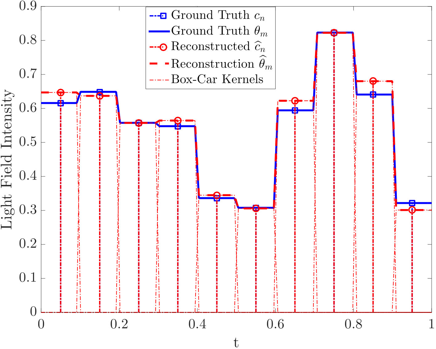 Figure 1
 Figure 2
 Figure 3
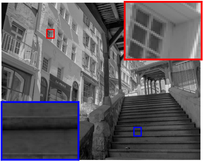 Figure 4
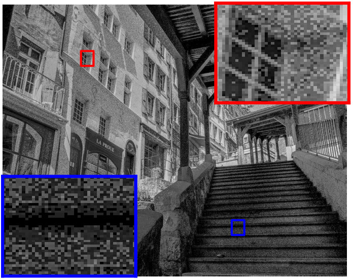 Figure 5
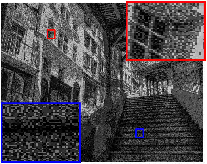 Figure 6
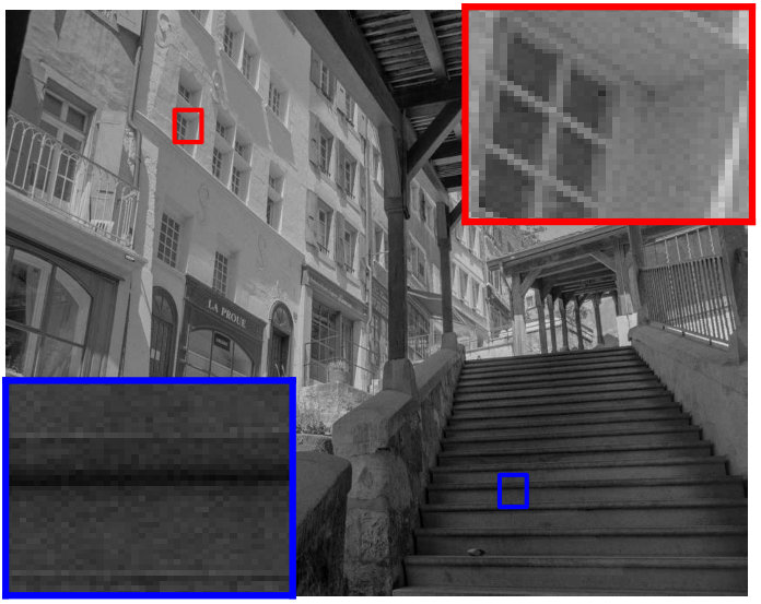 Figure 7
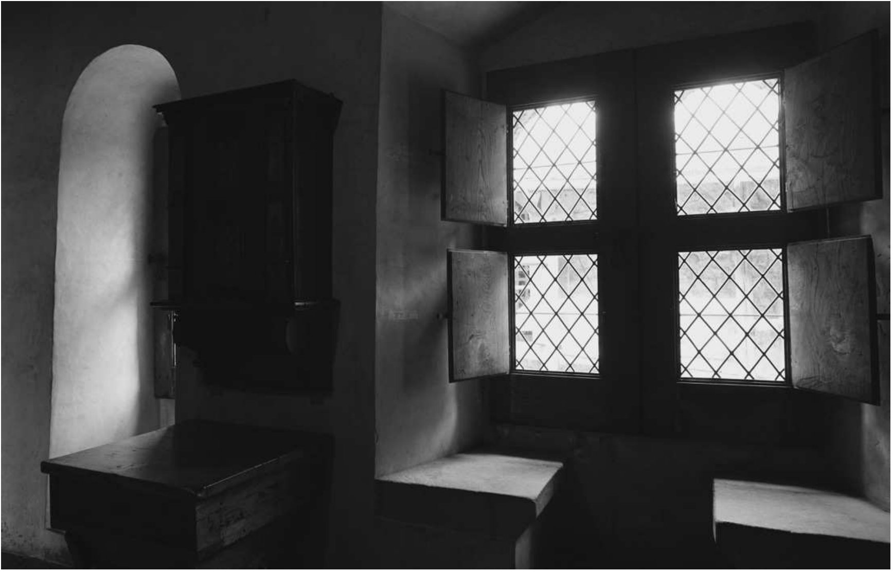 Figure 8
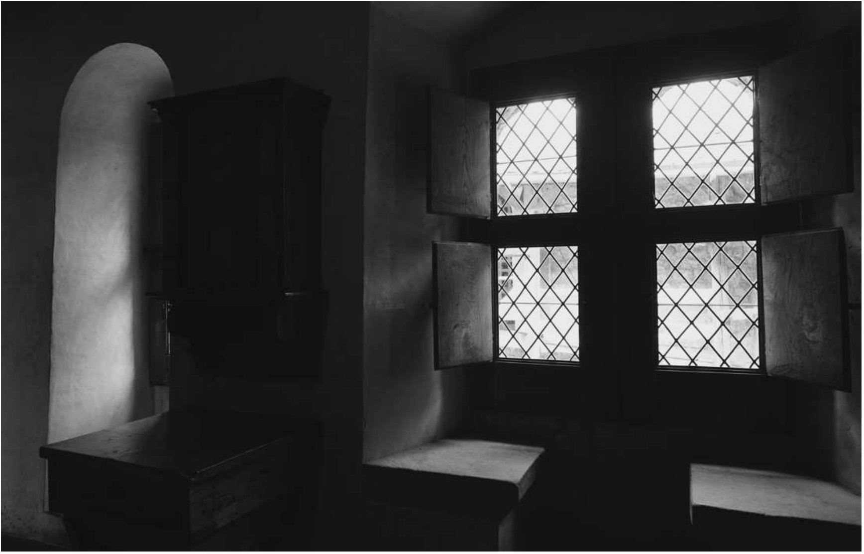 Figure 9
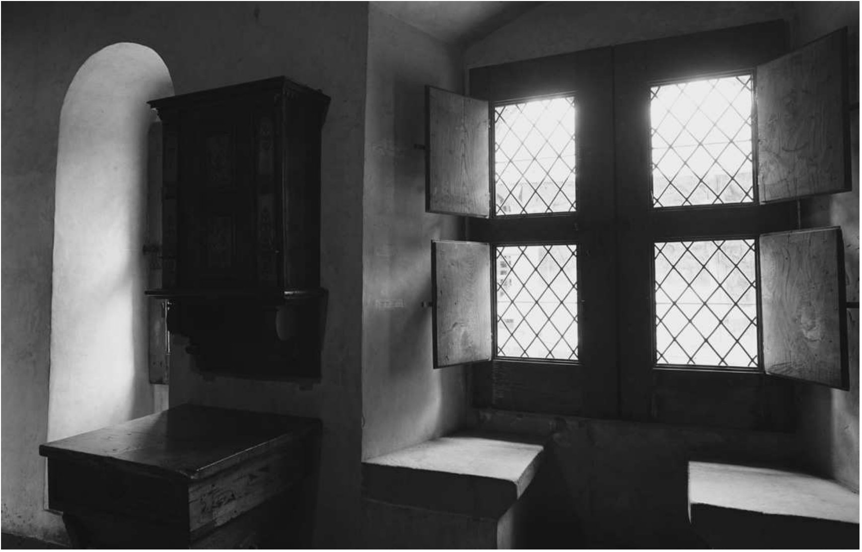 Figure 10
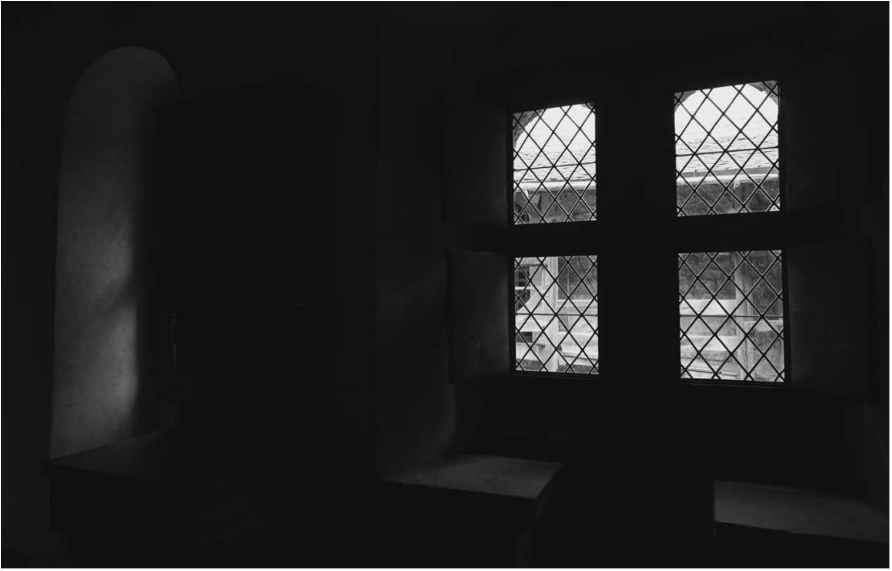 Figure 11
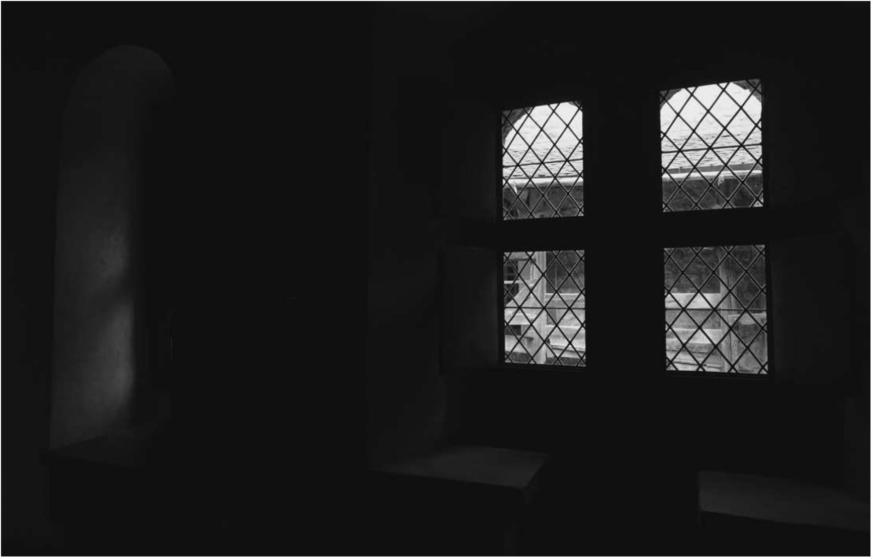 Figure 12
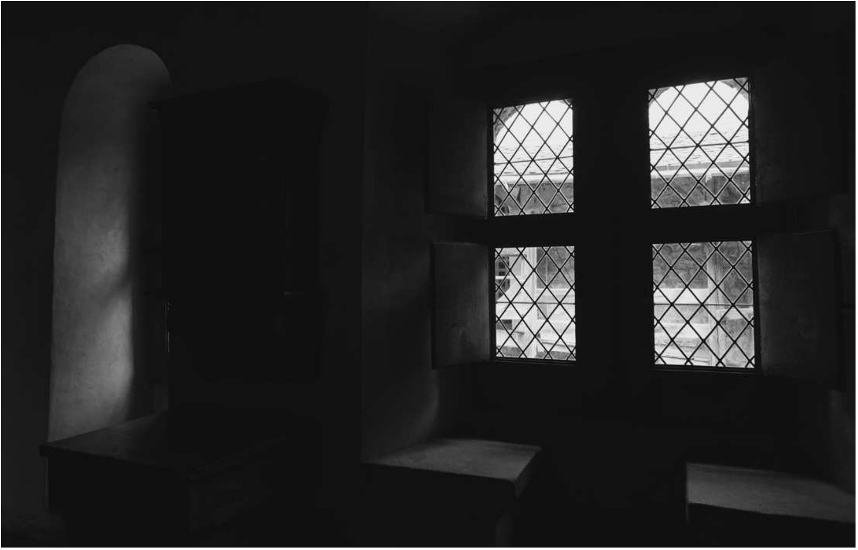 Figure 13
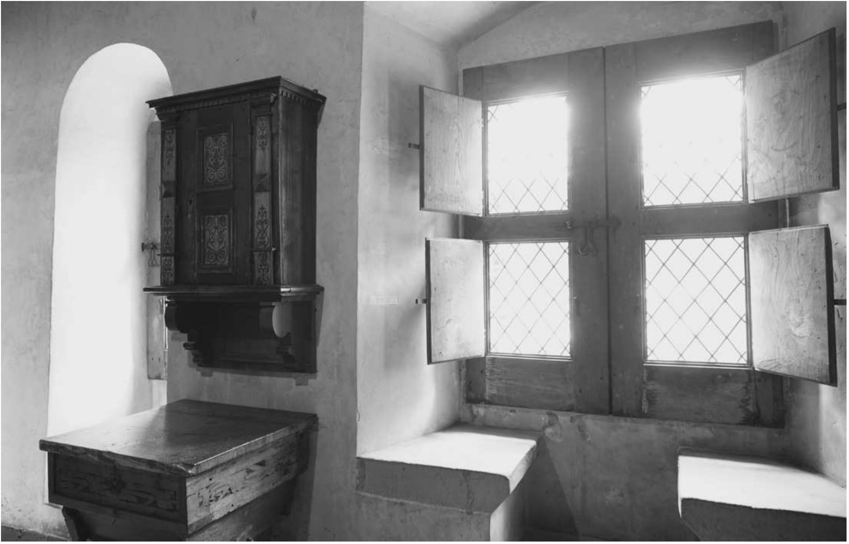 Figure 14
 Figure 15
 Figure 16
 Figure 17
 Figure 18
 Figure 19
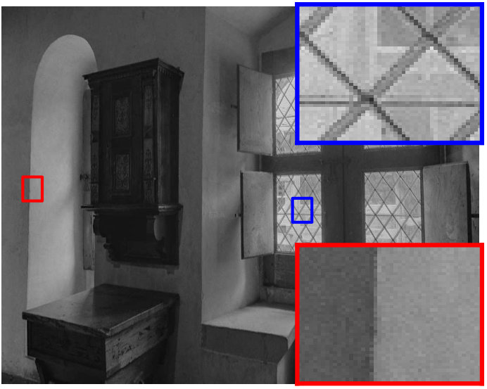 Figure 20
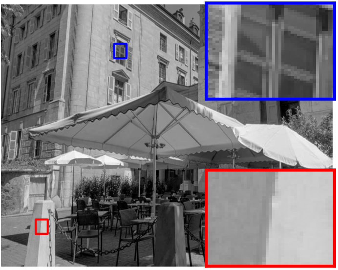 Figure 21
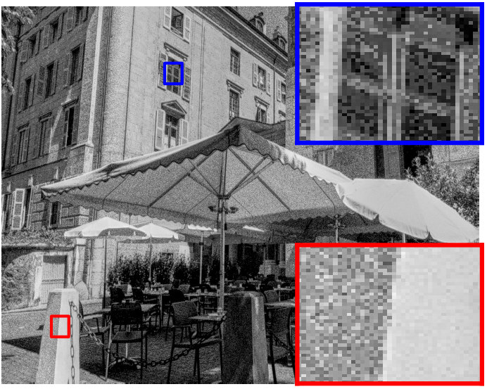 Figure 22
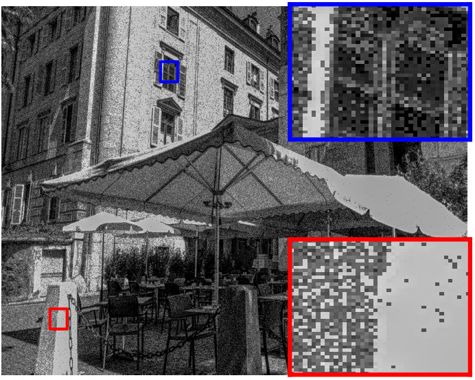 Figure 23
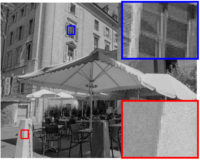 Figure 24
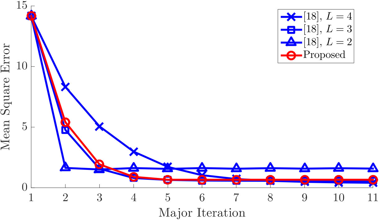 Figure 25
 Figure 26
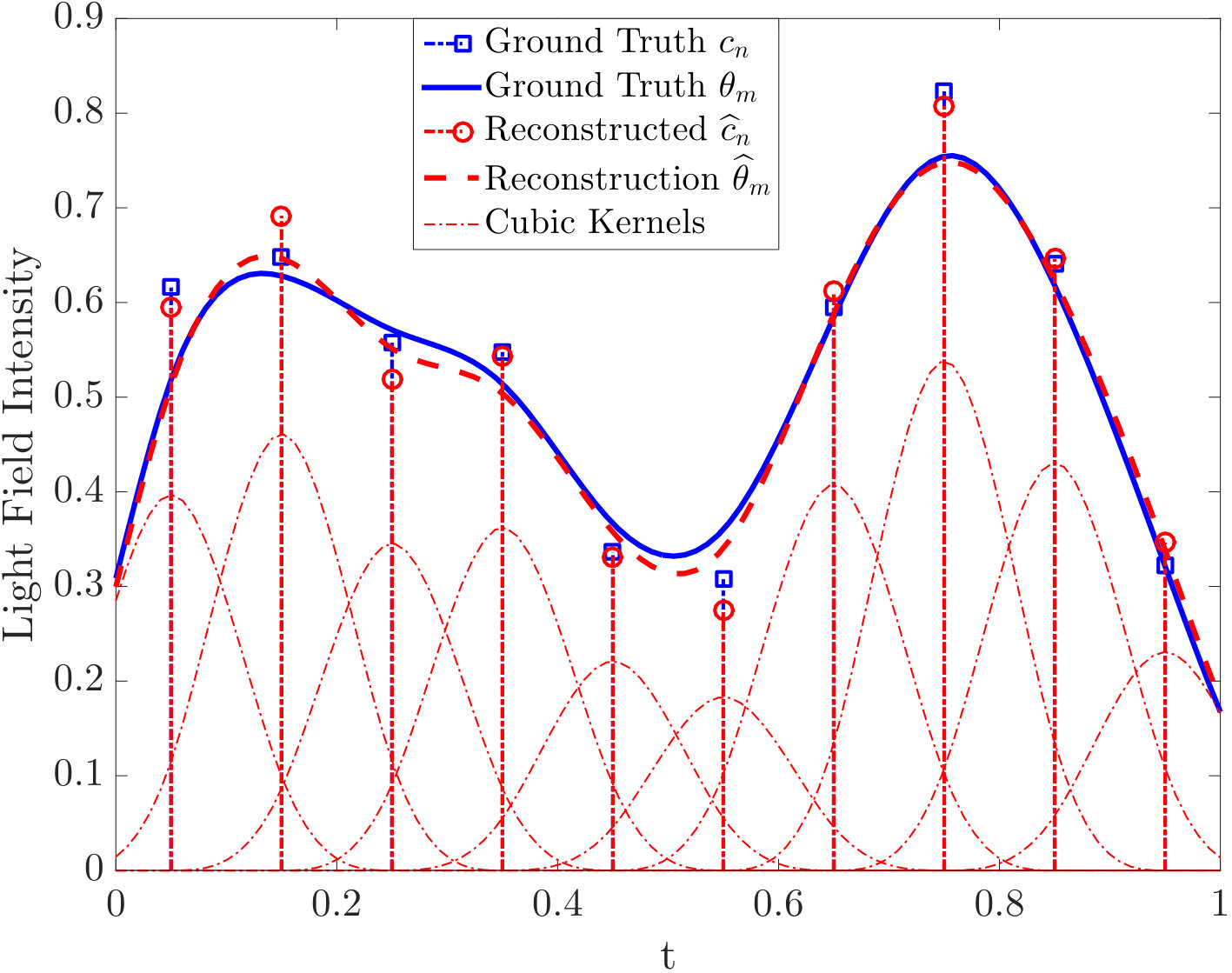 Figure 27
 Figure 28
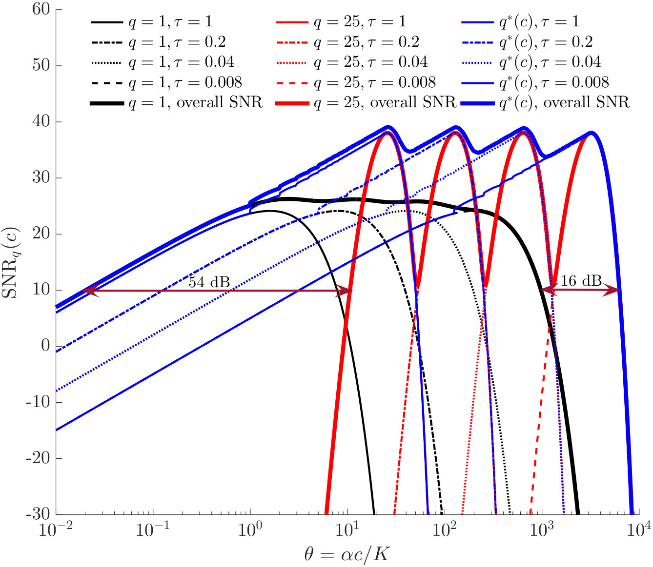 Figure 29
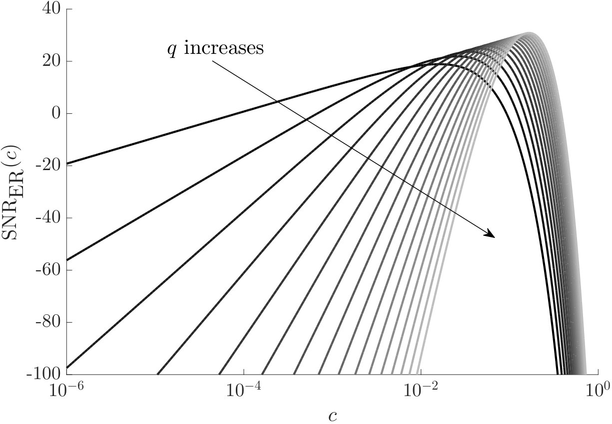 Figure 30
 Figure 31
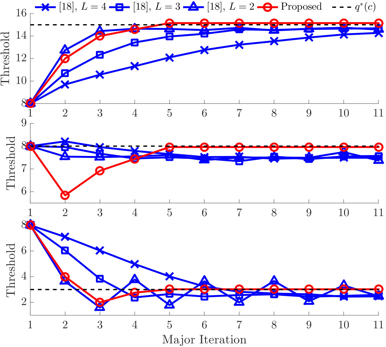 Figure 32
 Figure 33
 Figure 34
 Figure 35
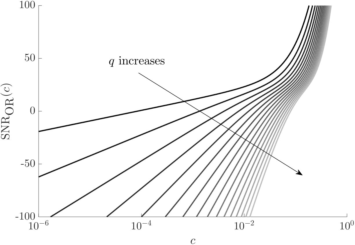 Figure 36
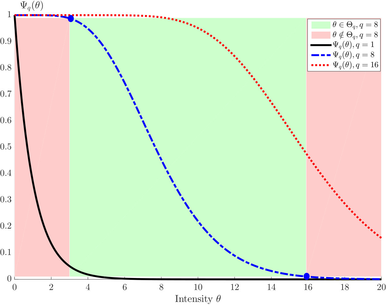 Figure 37
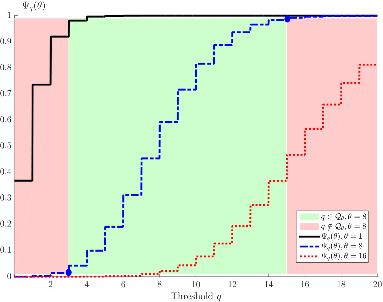 Figure 38
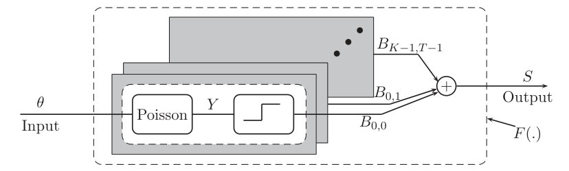 Figure 39
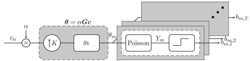 Figure 40
| Camera | Canon 5D CMOS | EMCCD [12] | GMAPD [13] | SPC SPAD [14] | SwissSPAD [11] | Fossum QIS [15] |
| Price | Prototype | Prototype | Prototype | Prototype | ||
| Resolution | ||||||
| Pixel Pitch (m) | 25 | 24 | ||||
| Full-well capacity | 69 ke- (@ISO100) | 180 ke- | - | e- | - | e- |
| Frames per second (fps) | 6 | |||||
| Sensor data rate | Mbps | 0.48 Gbps | 0.52 Gbps | 1.54 Gbps | 10.24 Gbps | 1 Gbps |
| Configuration |
|
Std | |||
|---|---|---|---|---|---|
| Uniform Threshold | 10.30 | 0.01 | |||
| 28.80 | 0.04 | ||||
| 23.22 | 0.02 | ||||
| 12.95 | 0.01 | ||||
| Conditional Reset [21] | Ascending sequence | 23.77 | 0.52 | ||
| Descending sequence | 24.95 | 0.53 | |||
| Proposed Method | 30.14 | 0.06 | |||
| 31.18 | 0.06 | ||||
| 32.78 | 0.02 |
Peer Reviews
No public reviews on file for this paper yet. If you reviewed it on a platform where reviews are public (OpenReview, ICLR, NeurIPS, ICML), you can paste yours below so the community can read it here.
Videos
No videos yet. Explain this paper in a talk, walkthrough, or lecture? Add one.
\reserveinserts
28
Optimal Threshold Design for Quanta Image Sensor
Omar A. Elgendy, and Stanley H. Chan The authors are with the School of Electrical and Computer Engineering, Purdue University, West Lafayette, IN 47907, USA. Email: { oelgendy, stanchan}@purdue.edu. The work was supported, in part, by the U.S. National Science Foundation under Grant CCF-1718007. A preliminary version of this paper was presented at the 2016 IEEE International Conference on Image Processing (ICIP), Phoenix, AZ.This paper follows the concept of reproducible research. All the results and examples presented in the paper are reproducible using the code and images available online at http://engineering.purdue.edu/ChanGroup/.
Abstract
Quanta Image Sensor (QIS) is a binary imaging device envisioned to be the next generation image sensor after CCD and CMOS. Equipped with a massive number of single photon detectors, the sensor has a threshold above which the number of arriving photons will trigger a binary response “1”, or “0” otherwise. Existing methods in the device literature typically assume that uniformly. We argue that a spatially varying threshold can significantly improve the signal-to-noise ratio of the reconstructed image. In this paper, we present an optimal threshold design framework. We make two contributions. First, we derive a set of oracle results to theoretically inform the maximally achievable performance. We show that the oracle threshold should match exactly with the underlying pixel intensity. Second, we show that around the oracle threshold there exists a set of thresholds that give asymptotically unbiased reconstructions. The asymptotic unbiasedness has a phase transition behavior which allows us to develop a practical threshold update scheme using a bisection method. Experimentally, the new threshold design method achieves better rate of convergence than existing methods.
Index Terms:
Quanta image sensor, single-photon imaging, high dynamic range, binary quantization, maximum likelihood.
I Introduction
I-A Threshold Design for Quanta Image Sensor
Quanta Image Sensor (QIS) is a class of solid-state image sensors envisioned to be the next generation imaging device after CCD and CMOS. Originally proposed by Eric Fossum in 2005 [1], the sensor has gained significant momentum in the past decade, both in terms of hardware design [2, 3, 4] and image processing [5, 6, 7, 8, 9]. The advantage of QIS over the mainstream CCD and CMOS is attributed to its high spatial resolution (e.g., pixels per sensor with nm pitch per pixel [10]) and high speed (e.g., 100k fps as reported in [11]). However, in order to simplify circuit, minimize power and reduce data transfer, QIS is operated in a binary mode: When the number of photons arriving at the sensor exceeds a threshold , the sensor generates a binary bit “1”. When the number of photons is less than , the sensor generates a “0”. The goal of this paper is to address the question of how to optimally choose to maximize the signal-to-noise ratio of the reconstructed image.
Optimal threshold design for QIS is important as it directly affects the dynamic range of an image. Figure 1 illustrates an example where we simulate the raw binary data acquired by a QIS using a uniform threshold . When is low, most of the bits in the raw input are “1”. The reconstructed image is therefore an over-exposed image. On the other hand, when is high, most of the bits in the raw input are “0”. The reconstructed image is then under-exposed. In both cases, it is evident from the simulation that a uniform threshold has limited performance. A better way is to allow to vary spatially so that a pixel (or a group of pixels) has its own threshold value. The result in Figure 1(d) shows the reconstruction result using a spatially varying threshold obtained from our proposed technique, which is clearly better than the uniform thresholds.
I-B Scope and Contributions
The goal of this paper is to present an optimal threshold design methodology and provide theoretical justifications. The two major contributions are summarized as follows.
First, we provide a rigorous theoretical analysis of the performance limit of the image reconstruction as a function of the threshold. These results form the basis of our subsequent discussions of the threshold update scheme. Some results are known, e.g., the signal-to-noise ratio is a function of the Fisher Information [16, 17], but a number of new results are shown. In particular, we show that (i) the maximum likelihood estimate has a closed-form expression in terms of the incomplete Gamma function (Section III.B); (ii) the oracle threshold can be derived in closed-form by maximizing the signal-to-noise ratio (Section III.C); (iii) the image reconstruction has a phase transition behavior (Section IV.A - Section IV.D).
Second, we propose an efficient threshold update scheme based on our theoretical results. The new scheme is a bisection method which iteratively updates the threshold without the need of reconstructing the image. By checking whether the proportion of one’s and zero’s approaches 0.5 in a spatial-temporal block, the threshold is guaranteed to be near optimal. Compared to other existing threshold update schemes such as [18] and [19, 20, 21], the new scheme offers significantly faster rate of convergence (Section IV.E). We also demonstrate how the dynamic range can be extended for high dynamic range (HDR) imaging (Section IV.F).
A preliminary version of this paper was presented in ICIP 2016 [8]. This journal version contains significantly more details including complete proofs of major results, more comprehensive comparisons with existing methods, and discussions of HDR imaging.
II Background
II-A Current State of QIS
Quanta Image Sensor (QIS) belongs to the family of photon-counting devices. These photon-counting devices have been known for a long time. Some better-known examples are the electron-multiplying charge-coupled device (EMCCD) [22, 23], single-photon avalanche diode (SPAD) [24, 14, 11], Geiger-mode avalanche photodiode (GMAPD) [13], etc. The common feature of these devices is their single photon sensitivity, which makes them useful in medical imaging [25, 26, 27], astronomy [28], defense [29], nuclear engineering [30], depth and reflectivity reconstruction [31], ultra-fast low-light tracking [32], and recently in quantum random number generation used in cryptography [33, 34].
The concept of QIS was first proposed by Fossum in 2005 as a solution for sub-diffraction limit pixels. The sensor was called the digital film sensor, and later the quanta image sensor [35, 36, 15]. After the introduction of QIS, researchers in EPFL developed a similar concept called the Gigavision camera [37, 38, 6]. Recently, teams at the University of Edingburgh [39, 14, 24] and EPFL [33, 40] have made new progresses in QIS using binary single photon detectors. In the industry, Rambus Inc. (Sunnyvale, CA) has developed binary image sensors for high dynamic range imaging [19, 20, 21]. Table I lists several recent QIS prototypes that are available or are currently being developed. As a comparison we also show a Canon 5D Mark III CMOS camera. Among many different features, the most noticeable is the frame rate. For example, SPS SPAD can be operated at 20k fps. SwissSPAD can even achieve 156k fps. Both are significantly faster than a standard CMOS camera.
II-B Related Work on Threshold Design
Existing work on QIS threshold design study can be summarized into three classes of methods.
- •
Markov Chain [18]. The Markov Chain method developed by Hu and Lu [18] is a time-sequential update scheme. A Markov Chain probability is used to control how easy the threshold should be increased or decreased. While the method has provable convergence, the threshold of each single photon detector of the QIS has to be updated sequentially in time. In contrast, our proposed method allows a group of single photon detectors to share the same threshold. As a result, our proposed method has significantly faster rate of convergence.
- •
Conditional Reset [19, 20, 21]. The conditional reset method is a hardware solution proposed by Vogelsang and colleagues. The idea is to take a sequence of images with ascending (or descending) thresholds, and digitally integrate the sequence to form an image. The drawback of the method, besides the additional hardware cost of the per-pixel reset transistors, is the limited quality of the reconstructed image. For the same number of frames, our proposed method produces better images.
- •
Checkerboard Threshold [16]. This method constructs a checkerboard of thresholds by alternating two threshold values and . The optimality criterion of and is based on minimizing the Cramér-Rao lower bound (CRLB) integrated over a range of light intensities, which is essentially an average case result. Our proposed method obtains the optimal threshold for each pixel. This per-pixel optimization has higher reconstruction performance compared to checkerboard threshold.
II-C QIS Imaging Model
In this subsection we provide an overview of the QIS imaging model. The model has been previously discussed in several papers, e.g., [6, 7, 8, 9]. Readers interested in details can refer to these papers for further explanations.
II-C1 Spatial Oversampling
We denote the discrete version of the light intensity as a vector , where specify the spatial coordinates. We assume that is normalized to the range for all so that there is no scaling ambiguity. To model the actual light intensity, we multiply by a constant to yield , where is a fixed scalar constant.
Given the -dimensional vector , QIS uses tiny pixels called jots to sample . The ratio is known as the spatial oversampling factor. The oversampling process is illustrated in Figure 2, where it first upsamples the vector by a factor of , and then filters the output by a lowpass filter . Mathematically, the process can be expressed as
[TABLE]
where denotes the light intensity sampled at the jots, and the matrix is defined as
[TABLE]
where is a vector of all ones and denotes the Kronecker product. Note that the choice of in (2) is the result of simplifying the model by assuming that the lowpass filter is for all . This assumption is typically reasonable, because on each QIS jot there is a micro-lens to focus the incident light. Although previous papers, e.g., [6, 7], do not make such assumption, in this paper we decide to use a simplified , for otherwise the theoretical analysis will become very complicated. Nevertheless, in the Supplementary Material we show comparison between a general and the simplified . The gap is usually insignificant.
II-C2 Truncated Poisson Process
We assume that the operating speed of QIS is significantly faster than the scene motion. Therefore, for a given scene (and also ), we are able to acquire a set of independent measurements. We illustrate this using the channels in Figure 2.
The oversampled signal generates a sequence of Poisson random variables according to the distribution
[TABLE]
where denotes the -th jot of the QIS and denotes the -th independent measurement in time. Denoting as the quantization threshold, the final observed binary measurement is a truncation of :
[TABLE]
The probability mass function of is given by
[TABLE]
The goal of image reconstruction is to recover the underlying image from the binary measurements . A pictorial illustration of the reconstruction is shown in Figure 3.
II-C3 Properties of Truncated Poisson Processes
The probability mass function of in (4) is Bernoulli. However, the right hand side of (4) involves infinite sums which are difficult to interpret. To simplify the equations, we consider the upper incomplete Gamma function defined in [41] as:
[TABLE]
where is the standard Gamma function. The incomplete Gamma function allows us to rewrite the infinite sums in (4) using the following identity [41]:
[TABLE]
Consequently, the probabilities in (4) become
[TABLE]
Example 1**.**
In the special case of , we obtain:
[TABLE]
which coincides with the results shown in [6] and [7].
The incomplete Gamma function is a decreasing function of because the first order derivative of with respect to is negative:
[TABLE]
The limiting behavior of is important. For a fixed , the function as and as . While still exists in these situations because is monotonically decreasing, for a given the value could be numerically very difficult to evaluate. To characterize the sets of and that is (numerically) invertible, we define the -admissible set and the -admissible set.
Definition 1**.**
The -admissible set and -admissible set of the incomplete Gamma function are
[TABLE]
respectively, where is a constant.
More discussions of the incomplete Gamma function can be found in the Supplementary Material.
Remark 1**.**
In this paper, we assume that QIS is noise-free, i.e., the only source of randomness is the truncated Poisson random variable. In real sensors, there will be readout noise, photo-response non-uniformity caused by conversion gain variation, dark count rate (a.k.a. dark current), optical crosstalk and electronic crosstalk. See [42] for details.
III Optimal Threshold: Theory
III-A Image Reconstruction by MLE
We begin the optimal threshold design by discussing image reconstruction because the optimality of the threshold is measured with respect to the reconstructed image. However, since QIS is a new device, the number of reconstruction methods is limited. A few examples that can be found in the literature are the gradient descent [6], dynamic programming [43], ADMM [7], and Transform-Denoise method [9], and neural network [44]. In this paper, we shall focus on the maximum likelihood estimation (MLE) approach as it provides closed-form expressions.
Given , MLE solves the following optimization problem:
[TABLE]
subject to the constraint that . Here, the right hand side of is the likelihood function of a Bernoulli random variable, and follows from taking the logarithm. With the defined in (2), we can partition into blocks where each block is
[TABLE]
Then, the pixel can be estimated as follows.
Proposition 1** (Closed-form ML Estimate).**
The solution of the MLE in (9) is
[TABLE]
where is the sum of bits in the -th block .
Proof.
See [9]. ∎
III-B Signal-to-Noise Ratio of ML Estimate
In order to determine the optimal threshold, we need to quantify the performance of the ML estimate. The performance metric we use is the signal-to-noise ratio of the ML estimate at every pixel . Considering each individually is allowed here because they are independently determined according to (10). For notation simplicity we drop the subscript in the subsequent discussions.
Definition 2**.**
The signal-to-noise ratio (SNR) of the ML estimate is defined as
[TABLE]
where the expectation is taken over the probability mass function of the binary measurements in (6).
The difficulty of working with is that it does not have a simple closed-form expression. In view of this, Lu [17] showed that the SNR is asymptotically linear to the log of the Fisher Information.
Proposition 2**.**
As ,
[TABLE]
where is the Fisher Information measuring the amount of information that the random variable carries about the unknown value .
Proof.
See [17]. ∎
While the asymptotic result shown in Proposition 2 has significantly simplified the SNR, we still need to determine the Fisher Information. The following proposition gives a new result of the Fisher Information with arbitrary .
Proposition 3**.**
The Fisher Information of the probability mass function in (6) under a threshold is:
[TABLE]
Proof.
See Appendix A-A. ∎
Substituting (13) into (12), we observe that the SNR can be approximated as
[TABLE]
which is characterized by the unknown pixel value , the threshold , the spatial oversampling ratio and the number of temporal measurements . To understand the behavior of (14), we show in Figure 4 as a function of for different thresholds . For a fixed , is a convex function with a unique maximum. The goal of optimal threshold design is to determine a which maximizes for a fixed .
Remark 2**.**
The in (14) can also be derived from a concept in the device literature called the exposure-referred SNR [45]. See Supplementary Material for discussions.
III-C Oracle Threshold
We now discuss the optimal threshold design in the oracle setting. We call the result oracle because the optimal threshold depends on the unknown pixel intensity . The practical threshold design scheme will be discussed in Section IV.
Using the definition of the signal-to-noise ratio, the optimal threshold is determined by maximizing with respect to :
[TABLE]
The second equality follows from Proposition 2. Substituting (13) yields an expression of the right hand side of (15). To further simplify the expression we derive the following lower bound.
Proposition 4**.**
The function is lower bounded as follows.
[TABLE]
Proof.
See Appendix A-B. ∎
Using this lower bound, we can derive the optimal threshold as follows 111Straightly speaking, the result shown in Proposition 5 is a “near-optimal” result because we are minimizing the lower bound. From our experience, the gap between the near-optimality and the exact optimality is typically insignificant..
Proposition 5**.**
The optimal threshold is
[TABLE]
where denotes the flooring operator that returns the largest integer smaller than or equal to the argument.
Proof.
See Appendix A-C. ∎
The result of Proposition 5 is important as it states that the oracle threshold is exactly the same as the light intensity . The flooring operation and the addition of a constant 1 are not crucial here because they are only used to ensure that is an integer. In [18], a special where was demonstrated experimentally. Proposition 5 now provides a theoretical justification.
IV Optimal Threshold: Practice
The oracle threshold derived in the previous section provides a theoretical foundation but is practically infeasible as it requires knowledge of the ground truth . In this section, we present an alternative solution by relaxing the optimality criteria. Our strategy is to consider a set of thresholds which are close to the oracle threshold , and show that they are asymptotically unbiased when the number of observed bits approaches infinity (Section IV.A). This result will allow us to characterize the estimate (Section IV.B). We will then show that there exists a phase transition region where the asymptotic unbiasedness is maintained as stays within a certain range around , and is lost rapidly as falls outside this range (Section IV.C - IV.D). Based on these observations, we will present a practical threshold update scheme (Section IV.E).
IV-A Asymptotic Unbiasedness
In order to derive an alternative threshold that does not require the ground truth, we start by reconsidering the ML estimate in Proposition 1. For a spatial-temporal block , the ML estimate satisfies the condition
[TABLE]
where is the sum of bits in . The right hand side of this equation is an important quantity. We denote it as
[TABLE]
In the device literature (e.g., [45]), the term is known as the bit-density as it is the proportion of ones in . Note that is a random variable because is the sum of i.i.d. random binary bits. Therefore, if we want to understand (17), we must first derive the the mean and variance of .
Proposition 6**.**
The mean and variance of are
[TABLE]
respectively.
Proof.
See Appendix A-D. ∎
We can now look at the asymptotic behavior of to see if it offers any insight about the optimal threshold. Applying the strong law of large number to , we can show that as ,
[TABLE]
Going back to (17)-(18), the ML estimate should have the expectation:
[TABLE]
where (a) follows from the definition of , (b) follows from (20), and (c) holds because and cancels each other.
What is the implication of (21)? It shows that the ML estimate is asymptotically unbiased. That is, as the number of independent measurements grows, the estimate approaches to the ground truth . In other words, as long as is large enough, the random variable would be an accurate estimate of the ground truth. How can this be used to determine the threshold ? Let us look at .
IV-B Set of Admissible Thresholds
The result in (17)-(21) shows that for a given (or equivalently ), the ML estimate can be found by
[TABLE]
When this happens, the given by (22) is asymptotically unbiased. However, the inversion is not always allowed. There is a set of ’s that can make invertible, which is defined as in Definition 1. The following proposition relates to .
Proposition 7**.**
Let be a constant. Then, for any
[TABLE]
the random variable will not attain 0 or 1 with probability at least , i.e.,
[TABLE]
In this case, the ML estimate is uniquely defined by (22).
Proof.
See Appendix A-E. ∎
Before we proceed, let us look at some rough magnitude of the parameters in the following example.
Example 2**.**
Let the ground truth pixel value be . The sensor parameters are set as , , . For a constant , the tolerance level is . Therefore, as long as , which is the set , the probability that equals to 0 or 1 is upper bounded by .
IV-C Gap between and
The result in the previous subsection shows that as long as , the ML estimate is asymptotic unbiased. However, how is a compared to the oracle threshold ? We answer this question in three parts.
First, does an asymptotically unbiased estimate maximize the SNR? The answer is no, because Proposition 5 states that if is the optimal threshold, then for any . Therefore, moving from the exact optimal to an asymptotically unbiased threshold is a relaxation of the optimality criteria.
If asymptotic unbiasedness is a relaxed optimality criteria, how much SNR drop will there be if we choose a but not necessarily ? We show in Figure 5 the plot of a typical experiment with setup discussed in Example 2. As shown in the figure, the green zone is the set , or equivalently . For any in this , the reconstruction has a SNR at least 30dB. If we further tighten so that , or equivalently , the SNR stays in the range , which is reasonably narrow.
How tight should be? Ideally we want to be as tight as possible. But knowing the fact that the incomplete Gamma function has a rapid transition (See the black line in Figure 5), can be much wider. In fact, we can choose such that stays close to 0.5, so that we are guaranteed to obtain a near optimal threshold. From an information theoretic point of view, is where the bit density attains the maximum information — if is too high then most bits become 0 whereas if is too low then most bits become 1. It is maximum when leads to 50% zeros and 50% ones. 222The exact optimal value of at is slightly lower than 0.5 due to the nonlinearity of the Gamma function. See Supplementary Material for additional discussion.
IV-D Phase Transition Phenomenon
We can now point out a very interesting phenomenon in Figure 5. In the upper plot of Figure 5 we show two sets of curves: blue curves (solid and dotted), and black curves (solid and dotted). The black curves represent the ratio , and the black curves represent the average bit density . For both sets of curves, we use dotted lines to illustrate the Monte-Carlo simulation using 10,000 random samples, where each sample refers to a spatial-temporal block containing binary bits. Notice that these dotted lines overlap exactly with their expectations, and hence (17)-(21) are valid.
Let us take a closer look at the blue curve . Let , where and are the smallest and the largest integers in respectively. There are three distinct phases:
When , the threshold is low and so most bits become 1. Therefore, and hence . Thus, as decreases.
When , the threshold high and so most bits become 0. Therefore, and hence . Thus, as increases.
When , the ML estimate is asymptotically unbiased. Therefore, .
Essentially, Figure 5 demonstrates a phase transition behavior of the threshold. Such phase transition exists because is only invertible when .
IV-E Bisection Threshold Update Scheme
Now we present a practical threshold update scheme. As we discussed in Section IV.C, the oracle threshold can be obtained when bit density is close to 0.5. Therefore, a practical procedure to determine is to sweep through a range of until the bit density reaches 0.5. To achieve this objective, we propose a bisection method illustrated in Figure 6 and Algorithm 1. Starting with initial thresholds and , we check whether the bit density satisfies and . If this is the case, then we find a mid point and check whether is greater or less than 0.5. If , we replace by , otherwise we replace by . The process repeats until is sufficiently close to 0.5.
In our proposed threshold update scheme, we assume that the image has been partitioned into blocks . Each contains binary bits and is used to estimate one pixel value . This setting results in different thresholds, one for every pixel. To generalize the setting, it is also possible to allow multiple pixels to share a common threshold. Figure 7 shows an example. The advantage of sharing a threshold for multiple pixels is that circuits associated with the sensor can be simplified. In terms of performance, since neighboring pixels are typically correlated, sharing the threshold causes little drop in the resulting SNR.
The price that the proposed bisection algorithm has to pay is the number of frames it requires to determine a good . For every evaluation of , the sensor has to physically acquire one frame and compute the bit density in each of the blocks. Therefore, the more bisection steps we need, the more frames that the sensor has to physically acquire. The rate of convergence of the proposed method and existing methods will be compared in Section V.
IV-F Extension to High Dynamic Range
While QIS is a photon counting device, it is designed to count a few photons to keep the full-well capacity small, e.g. 20 photoelectrons as reported in [46]. Therefore, for practical imaging tasks, we need to extend the dynamic range for QIS.
There are two ways to enable dynamic range extension:
- •
Bright Scenes: Reduce Duty Cycle. In the signal processing block diagram shown in Figure 2, we can replace the constant by a fraction as , where determines the ratio between the actual integration time and the readout scan time. It can also be referred to the shutter duty cycle because the shutter is opened to collect photons during this proportion of time [47]. For very bright scenes, a low duty cycle will prevent QIS from saturating early.
- •
Dark Scenes: Multiple Measurements. For dark scenes, multiple measurements can be taken to ensure enough photons over the measurement period. This, however, is different from conventional HDR imaging. In conventional HDR imaging, the multiple shots are taken at different shutter speeds, e.g., 1/8192, 1/2048, 1/512, 1/128, 1/32, 1/8, 1/2 seconds [48], which is redundant. QIS’s multiple shot functions more similar to burst photography [49]. The amount of acquisition time is significantly less than the conventional HDR imaging.
These two methods can be used for any threshold scheme, including ours and others. The benefit of using our proposed threshold scheme is that it supports a much wider dynamic range extension. In Figure 8, we illustrate the total dynamic range that can be covered using 4 multiple measurements at duty cycles , , , and . The maximum threshold level is , and the minimum threshold level is . It can be seen from the figure that with the optimal threshold , the dynamic range is significantly more than the non-optimal ones. In particular, we observe a 16dB and a 54dB improvement compared to and , respectively. Experimental results will be shown in Section V.C.
IV-G Hardware Consideration
Concerning the hardware implementation, we anticipate that future QIS will be equipped with per-pixel FPGAs to perform the proposed threshold update scheme. On-sensor FPGA is an actively developing technology. For example, MIT Lincoln Lab’s digital focal plane array can achieve on-sensor image stabilization and edge detection [50] . For QIS threshold update, the complexity is low because we are only counting the number of ones in the bisection. More specifically, in order to perform the bisection, we only need additions to compute ; one comparison ; one addition and one multiplication (with a constant 0.5) to update the threshold . The dominating factor here is the additions, which can be implemented efficiently by shifting bits in a buffer.
We should also point out that the proposed bisection method can be flexibly adjusted spatially and temporally for different hardware configurations. For example, we can use a spatial-temporal window for low-resolution high-speed imaging, or for high-resolution low-speed imaging. This flexibility offers additional advantages of QIS over conventional CCD and CMOS cameras.
V Experimental Results
In this section we evaluate the proposed threshold update scheme by comparing it with existing methods. We consider two evaluation metrics: (1) convergence rate of the threshold update methods; (2) quality of the reconstructed images. For reconstruction evaluation, we create our own Purdue dataset comprising 77 images captured by a Canon EOS Rebel T6i camera. For HDR imaging, we use the HDR-Eye dataset by Nemoto et al. [51, 52]. In all experiments, we fix the spatial over-sampling factor as , and number of temporal frames as . The maximum threshold level is set as to ensure that it is realistic for today’s QIS.
V-A Convergence
We compare the proposed threshold update scheme with the Markov Chain (MC) adaptation proposed by Hu and Lu [18]. The Markov Chain adaptation models the threshold as a variable with states. These states can be regarded as steps before reaching to the next threshold level. The probability of changing from one state to another is controlled by a parameter with . When a bit arrives, the state will be updated (increased or decreased) or will remain unchanged. Once the state is increased by times, the threshold will be increased by one.
When comparing Markov Chain adaptation with the proposed bisection algorithm, one should be aware of the difference between the two methods. Markov Chain adaptation is a per-jot update scheme whereas the proposed bisection algorithm is a per-pixel update scheme. For a pixel with jots, Markov Chain adaptation needs iterations to update the threshold sequentially. In contrast, the proposed bisection algorithm updates a common threshold for all jots simultaneously. Thus in practice our bisection algorithm is significantly less complex to implement in hardware than the Markov Chain. In order to take the different forms of updates into account, we treat the iterations of Markov Chain adaptation as one “major iteration” and compare it with the one bisection step of the proposed algorithm.
The first comparison we make is to check the threshold at different jots. Figure 9 shows the results of three typical runs with underlying optimal thresholds . In this experiment, we generate 100 random binary blocks of size and estimate the threshold at each major iteration. We report the average of these 100 estimates to minimize the randomness of the data. The results show that one iteration of the proposed bisection algorithm works as good as the iterations of the Markov Chain adaptation. In some cases, Markov Chain tends to oscillate whereas the bisection result is stable.
The second comparison we make is to check how close the estimated threshold is compared to the optimal threshold. The optimal threshold is obtained using the oracle scheme. In Figure 10, we plot the mean squared error between the estimated threshold and the oracle threshold. For fairness, we show the results of the MSE averaged over the 77 images of our dataset, and 50 random samples per image. One threshold is shared by jots, and each jots correspond to one pixel. The result is consistent with the ones shown in Figure 9.
V-B Image Reconstruction Quality
The convergence comparison in the previous subsection is only useful to compare threshold update methods that actually return a threshold. In the QIS literature, there are methods that implicitly update the threshold, e.g., the conditional reset method [21]. For comparison with these methods, we have to compare the quality of the image reconstructed from the binary raw data. The image reconstruction is done using the closed-form ML estimate in Section III-A.
We consider three classes of methods:
- •
Uniform Threshold. Uniform threshold is commonly used in the device literature [5, 6, 7]. A uniform threshold is a single threshold applied to all pixels in the image. In this experiment, we consider the following choices of uniform thresholds: , , and .
- •
Conditional Reset [21]. Conditional reset counts the number of photons and is reset when it is above the threshold. The threshold in conditional reset is sequentially increasing or decreasing. The reconstructed image is obtained by digitally integrating the raw binary frames.
- •
Proposed Method. As we discussed in Section IV-E, the proposed method can be implemented to let multiple pixels share a common threshold. Thus, in this experiment we consider three sharing strategies: (1) Share a threshold between a neighborhood of jots (i.e., one threshold for one pixel); (2) Share a threshold between a neighborhood of jots (i.e., one threshold for pixel); (3) Share a threshold between a neighborhood of jots (i.e., one threshold for pixels).
The result of the experiment is shown in Table II. The PSNR values reported are averaged over 77 images in our dataset. Each image generates 50 random realizations, and the PSNR of an image is averaged over these 50 random realizations to minimize the randomness. As shown in the table, while conditional reset generally performs better than a uniform threshold, it performs significantly worse than the proposed threshold update scheme.
V-C Influence of QIS Threshold on HDR Imaging
Since QIS does not have sufficient full well capacity to accumulate photons for HDR imaging, we apply the dynamic range extension method discussed in Section IV-F. When different threshold schemes are used, the reconstructed HDR images will be affected. The objective of this experiment is to evaluate the influence of the threshold in HDR imaging.
In this experiment, we consider the HDR-Eye image dataset [51, 52]. Each HDR image in this dataset contains 9 images acquired at different exposure settings (,, , , [math], , , , and EV). A snapshot of these images are shown in Figure 11. From each exposure, we simulate the photon counts resulting from the luminance channel. The sensor gain is set as to ensure proper number of photons, where and . On the reconstruction side, we reconstruct the 9 images using the MLE discussed in Section III-A. Tone mapping and exposure fusion [53] are applied to the 9 imags to generate an HDR image. As a reference, we apply the same tone mapping and fusion algorithm to the 9 ground truth images. PSNR between the reference and the estimated is then recorded.
The result of this experiment is shown in Figure 12. With the proposed threshold update scheme, the reconstructed images achieve the highest PSNR value and visual quality. When , which is too low, the image appears under-exposed. When , which is too high, the image appears over-exposed. The spatially varying property of the proposed method mitigates the issue by allowing multiple thresholds.
In practice, one would typically add image denoisers to handle the randomness in the ML estimate and potentially other types of noise. This can be done using methods such as [9]. In HDR literature, there are also optical approaches that reduce the number of exposures, e.g., [54, 55]. These techniques are complementary to QIS, because QIS is a sensor of similar functionality of a CMOS. Thus optical techniques can always be added.
VI Conclusion
Quanta Image Sensor is a new image sensor for high speed, high resolution and high dynamic range imaging. The sensor has a threshold which needs to be carefully adjusted so that the dynamic range can be maximized. We studied the threshold design problem by establishing several theoretical results. First, we showed that an oracle threshold can be obtained assuming that we know the underlying pixel value. Our result showed that the oracle threshold must match with the pixel value in order to maximize the signal-to-noise ratio. Second, we showed that around the oracle threshold, there exists a set of thresholds that can produce asymptotically unbiased estimates of the pixel value. Within this set of threshold, the signal-to-noise ratio stays very close to the oracle case. Third, we developed a bisection method to update the threshold scheme. We also discussed how QIS can be used in HDR imaging, and its advantages compared to standard sensors. Experimental results showed the effectiveness of our proposed approach compared to the standard approach that uses uniform threshold for all pixels.
Acknowledgment
The authors thank Professor Eric Fossum, Jiaju Ma and Saleh Masoodian at Dartmouth College for many insightful discussions about the physics and circuits of QIS.
Appendix A
A-A Proof of Proposition 3
The Fisher Information metric is defined as:
[TABLE]
where . Using the chain rule, we can derive the Fisher Information as follows
[TABLE]
The expectation can be calculated as follows
[TABLE]
Using (7) to differentiate the 1st term, we get:
[TABLE]
where and . Similarly, the second term is
[TABLE]
Substitute (A-A) and (LABEL:eq:partial0) in (A-A) yields
[TABLE]
A-B Proof of Proposition 4
The lower bound is obtained by observing that the product attains its maximum value when . Substituting with the upper bound , we get:
[TABLE]
A-C Proof of Proposition 5
Using the definition of Gamma function and , we can rewrite the lower bound in Proposition 4 as follows.
[TABLE]
The only dependence on is in the second term, so we take a closer look at it. When , all summands are positive because . Hence, the total sum increases by increasing . On the other hand, when , we start to add negative summands because . Therefore, the total sum decreases on increasing over . Thus, maximum is obtained at .
A-D Proof of Proposition 6
By definition, is the summation of independent i.i.d. Bernoulli random variables. Therefore, is a binomial random variable with parameters and . The mean and variance of a binomial random variable is , and . Therefore, we have
[TABLE]
A-E Proof of Proposition 7
The probability can be evaluated by checking the complement when or :
[TABLE]
where (a) follows from the fact that , which is a sum of i.i.d. Bernoulli random variables, is a binomial random variable.
Let . If
[TABLE]
then we have
[TABLE]
Thus, it holds that
[TABLE]
The reference list from the paper itself. Each links out to its DOI / PubMed record.
- 1[1] E. R. Fossum, “What to do with sub-diffraction-limit (SDL) pixels?–A proposal for a gigapixel digital film sensor (DFS),” in Proc. IEEE Workshop CC Ds Adv. Image Sensors , Sep. 2005, pp. 214–217.
- 2[2] J. Ma, D. Hondongwa, and E. R. Fossum, “Jot devices and the quanta image sensor,” in Proc. IEEE Int. Electron Devices Meeting , Dec. 2014, pp. 10.1.1–10.1.4.
- 3[3] J. Ma and E. R. Fossum, “A pump-gate jot device with high conversion gain for a quanta image sensor,” IEEE J. Electron Devices Soc. , vol. 3, no. 2, pp. 73–77, Mar. 2015.
- 4[4] J. Ma, L. Anzagira, and E. R. Fossum, “A 1 μ 𝜇 \mu m-pitch quanta image sensor jot device with shared readout,” IEEE J. Electron Devices Soc. , vol. 4, no. 2, pp. 83–89, Mar. 2016.
- 5[5] F. Yang, Y. M. Lu, L. Sbaiz, and M. Vetterli, “An optimal algorithm for reconstructing images from binary measurements,” in Proc. IS&T/SPIE Electronic Imaging, Computational Imaging VIII , Jan. 2010, vol. 7533, pp. 75330 K–75330 K–12.
- 6[6] F. Yang, Y. M. Lu, L. Sbaiz, and M. Vetterli, “Bits from photons: Oversampled image acquisition using binary poisson statistics,” IEEE Trans. Image Process. , vol. 21, no. 4, pp. 1421–1436, Apr. 2012.
- 7[7] S. H. Chan and Y. M. Lu, “Efficient image reconstruction for gigapixel quantum image sensors,” in Proc. IEEE Global Conf. Signal and Information Processing (Global SIP’14) , Dec. 2014, pp. 312–316.
- 8[8] O. A. Elgendy and S. H. Chan, “Image reconstruction and threshold design for quanta image sensors,” in Proc. IEEE Int. Conf. Image Process. (ICIP’16) , Sep. 2016, pp. 978–982.