Made-to-measure modeling of observed galaxy dynamics
Jo Bovy, Daisuke Kawata, Jason A. S. Hunt

TL;DR
This paper enhances the made-to-measure (M2M) dynamical modeling technique, enabling simultaneous optimization of system parameters and uncertainties, demonstrated through galaxy data and a harmonic oscillator model.
Contribution
The authors introduce improvements to the M2M method, including simultaneous parameter optimization and a sampling approach for uncertainty quantification in galaxy dynamics modeling.
Findings
Improved M2M method allows joint optimization of nuisance and potential parameters.
Demonstrated the method with Gaia DR1 data on F-type stars.
Enabled probabilistic modeling of system uncertainties.
Abstract
Among dynamical modeling techniques, the made-to-measure (M2M) method for modeling steady-state systems is among the most flexible, allowing non-parametric distribution functions in complex gravitational potentials to be modeled efficiently using N-body particles. Here we propose and test various improvements to the standard M2M method for modeling observed data, illustrated using the simple setup of a one-dimensional harmonic oscillator. We demonstrate that nuisance parameters describing the modeled system's orientation with respect to the observer---e.g., an external galaxy's inclination or the Sun's position in the Milky Way---as well as the parameters of an external gravitational field can be optimized simultaneously with the particle weights. We develop a method for sampling from the high-dimensional uncertainty distribution of the particle weights. We combine this in a Gibbs…
Click any figure to enlarge with its caption.
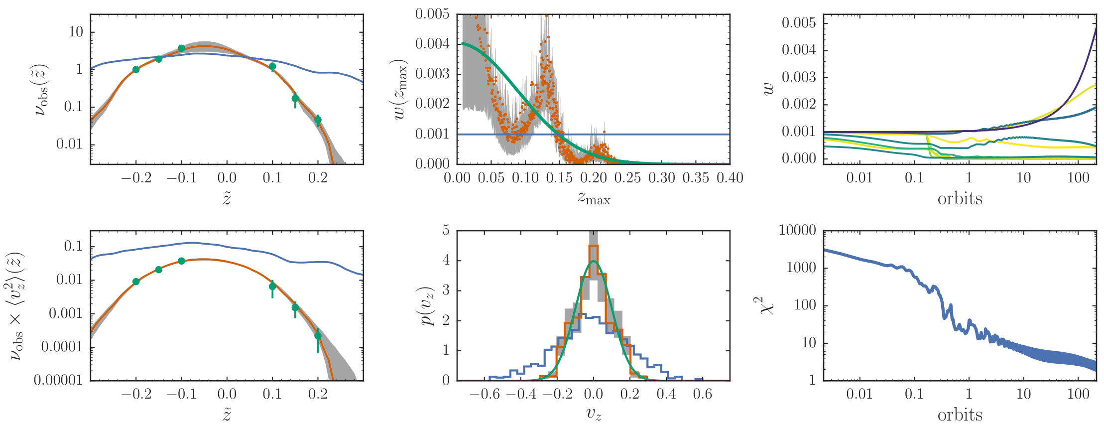 Figure 1
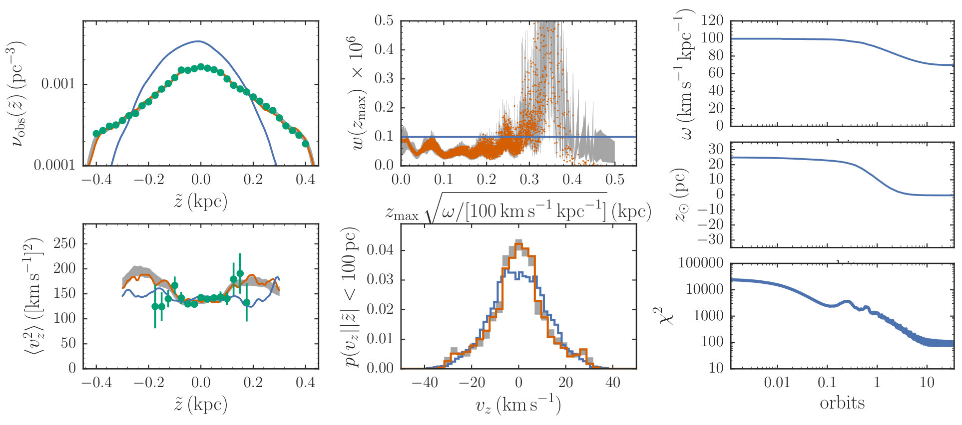 Figure 2
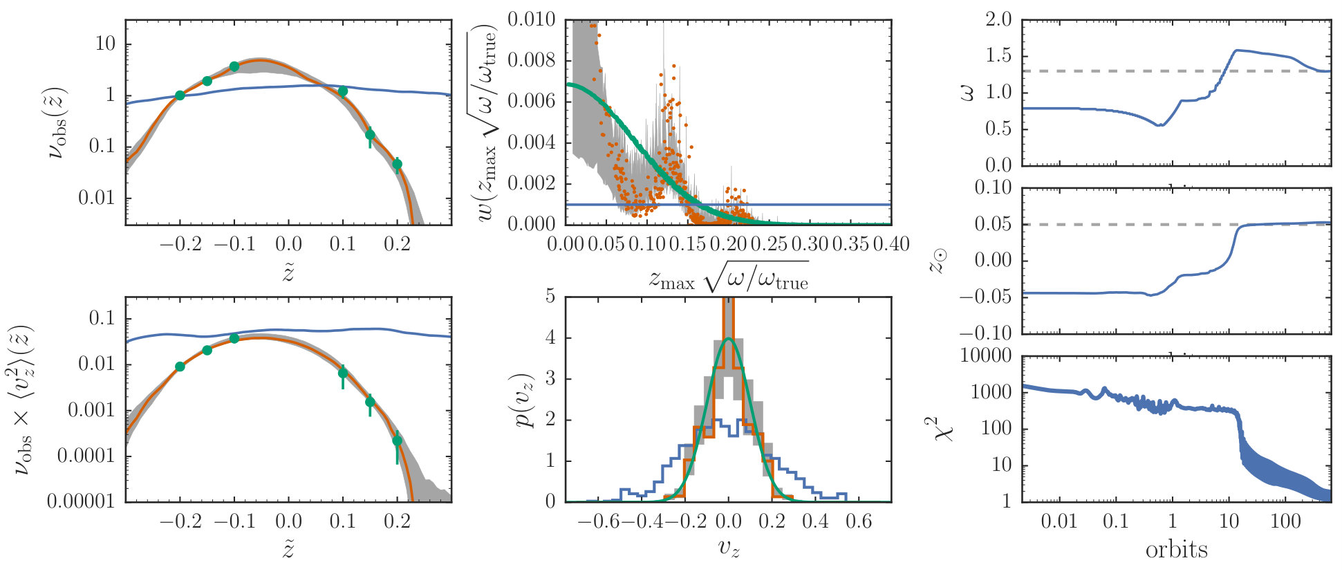 Figure 3
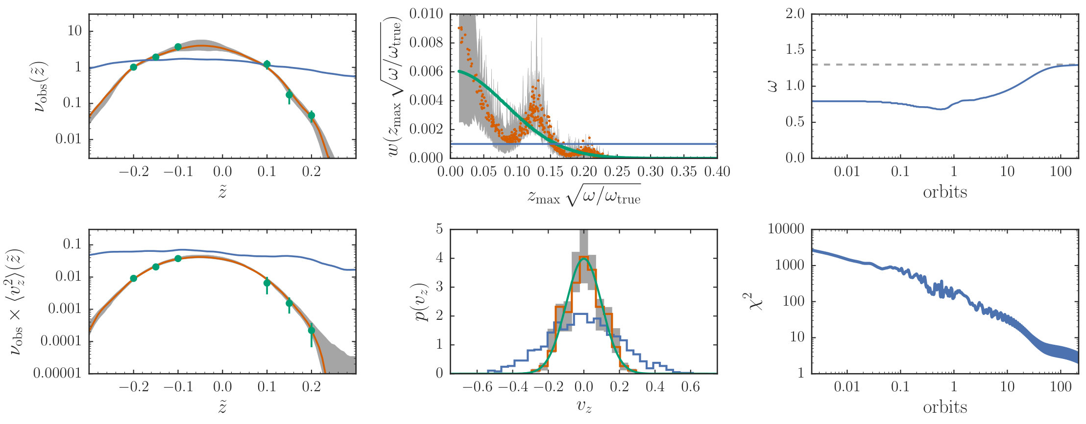 Figure 4
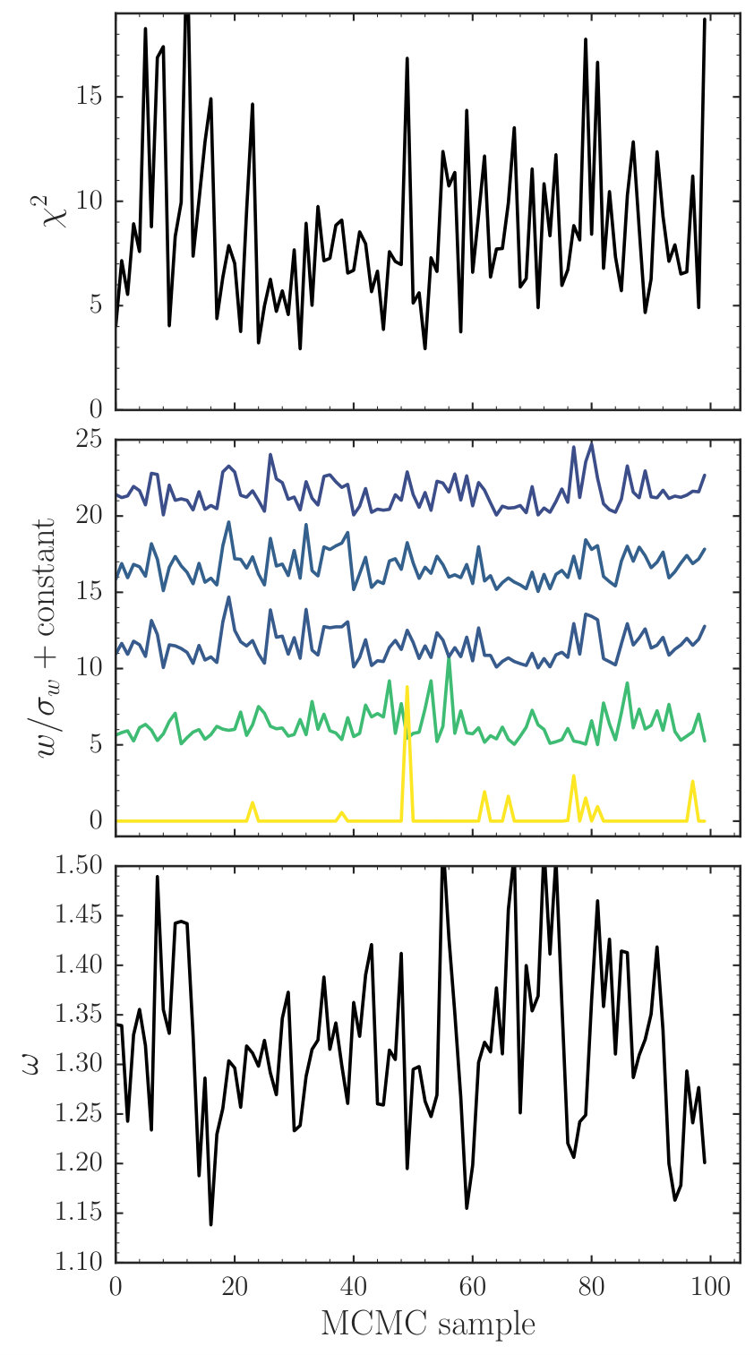 Figure 5
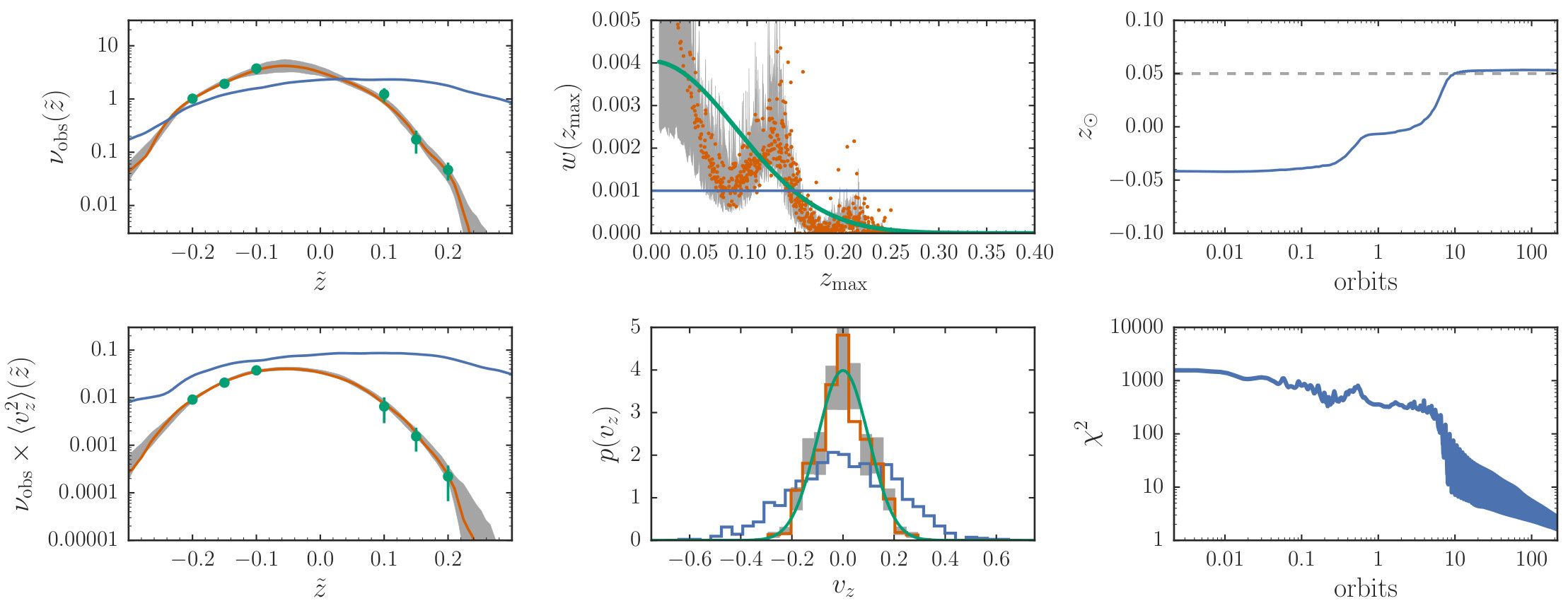 Figure 6
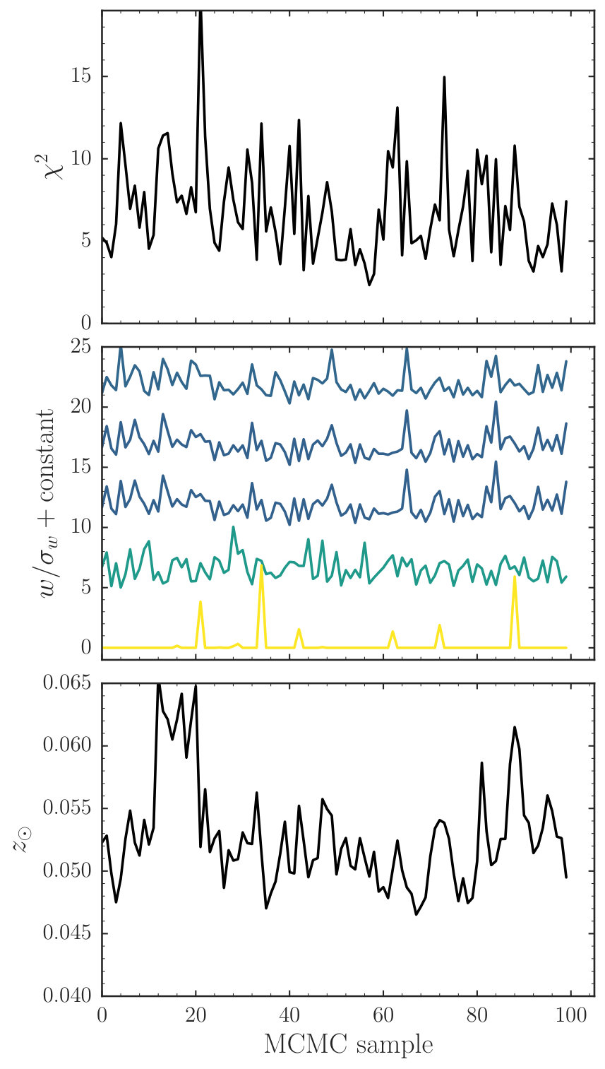 Figure 7
Peer Reviews
No public reviews on file for this paper yet. If you reviewed it on a platform where reviews are public (OpenReview, ICLR, NeurIPS, ICML), you can paste yours below so the community can read it here.
Videos
No videos yet. Explain this paper in a talk, walkthrough, or lecture? Add one.
Made-to-measure modeling of observed galaxy dynamics
Jo Bovy1,2, Daisuke Kawata3, & Jason A. S. Hunt4
1Department of Astronomy and Astrophysics, University of Toronto, 50 St. George Street, Toronto, ON M5S 3H4, Canada
2Center for Computational Astrophysics, Flatiron Institute, 162 5th Ave, New York, NY 10010, USA
3Mullard Space Science Laboratory, University College London, Holmbury St. Mary, Dorking, Surrey, RH5 6NT, United Kingdom
4Dunlap Institute for Astronomy and Astrophysics, University of Toronto, 50 St. George Street, Toronto, Ontario, M5S 3H4, Canada E-mail: [email protected] P. Sloan Fellow
(6 September 2017)
Abstract
Among dynamical modeling techniques, the made-to-measure (M2M) method for modeling steady-state systems is among the most flexible, allowing non-parametric distribution functions in complex gravitational potentials to be modeled efficiently using -body particles. Here we propose and test various improvements to the standard M2M method for modeling observed data, illustrated using the simple setup of a one-dimensional harmonic oscillator. We demonstrate that nuisance parameters describing the modeled system’s orientation with respect to the observer—e.g., an external galaxy’s inclination or the Sun’s position in the Milky Way— as well as the parameters of an external gravitational field can be optimized simultaneously with the particle weights. We develop a method for sampling from the high-dimensional uncertainty distribution of the particle weights. We combine this in a Gibbs sampler with samplers for the nuisance and potential parameters to explore the uncertainty distribution of the full set of parameters. We illustrate our M2M improvements by modeling the vertical density and kinematics of F-type stars in Gaia DR1. The novel M2M method proposed here allows full probabilistic modeling of steady-state dynamical systems, allowing uncertainties on the non-parametric distribution function and on nuisance parameters to be taken into account when constraining the dark and baryonic masses of stellar systems.
keywords:
galaxies: general — galaxies: kinematics and dynamics — galaxies: fundamental parameters — galaxies: structure — Galaxy: kinematics and dynamics — solar neighborhood
††pagerange: Made-to-measure modeling of observed galaxy dynamics–LABEL:LastPage††pubyear: 2017
1 Introduction
Constraining the orbital structure and mass distribution of astrophysical systems through dynamical modeling is one of the fundamental ways to learn about the dark-matter and baryonic distribution in external galaxies (e.g., Rix et al., 1997; Cappellari et al., 2012), supermassive black holes at the centers of galaxies (e.g., Magorrian et al., 1998), and the mass distribution of the Milky Way (e.g., Bovy & Rix, 2013), to name but a few. Of particular interest are systems—such as galaxies or star clusters—that may be assumed to be in a steady state. Many techniques have been proposed to model such systems, typically combining the steady-state assumption with further assumptions about the orbital structure (e.g., the velocity anisotropy) or symmetry (e.g., spherical or axisymmetric) of the system. The simplest among these techniques are those based on moments of the collisionless Boltzmann equation, e.g., the Jeans equations, which despite their restrictive assumptions remain a useful tool for interpreting data (e.g., Cappellari et al., 2013). A second class of techniques directly uses parameterized distribution functions (DFs) that satisfy the collisionless Boltzmann equation by only depending on integrals of the motion. While restricted to gravitational potentials for which such integrals can be computed, this class of models has reached a high level of sophistication, especially in the Milky Way (e.g., Binney, 2010; Bovy & Rix, 2013; Trick et al., 2016). A third class of methods eschews parameterized DFs, but rather builds a steady-state model in a fixed gravitational potential from a large number of orbit building blocks with weights determined by fitting a set of constraints (Schwarzschild, 1979, 1993).
Syer & Tremaine (1996) proposed a method known as made-to-measure (M2M) modeling that is closely related to orbit-based modeling. In M2M, the DF is represented not by entire orbits but instead by a set of -body particles with positions and velocities and weights . They demonstrated that a steady-state solution to a set of constraints on the phase-space distribution (expressed as a ,the mean-squared difference between the model and the data) can be obtained by slowly adjusting the weights of each particle in the direction of decreasing while integrating the orbits of the particles. The advantages of this particle-based technique over orbit-based methods are that only the current snapshot needs to be stored in memory rather than entire orbits, that the -body particles can contribute a self-consistent part of the gravitational potential, and that one ends up with an actual sampling from the steady-state DF. The latter makes M2M also an ideal technique for initializing -body simulations (e.g., Dehnen, 2009; Malvido & Sellwood, 2015).
Since its original description, various improvements have been made to the basic M2M setup, such as allowing for observational uncertainties and kinematic data in the constraints (De Lorenzi et al., 2007; Long & Mao, 2010), integrating particles on individual time scales for problems with a range of orbital frequencies (Dehnen, 2009), improvements in the smoothing applied to the model (Dehnen, 2009), and allowing data for individual stars as constraints (Hunt & Kawata, 2013; Hunt et al., 2013; Hunt & Kawata, 2014). As currently conceived, M2M modeling applies to the particle weights only and any other parameter describing the system is held fixed during the optimization. This includes nuisance parameters describing the modeled system’s orientation with respect to the observer, for example, the inclination of an external galaxy or the Sun’s distance to the Galactic center for Milky-Way applications, and the parameters of the external gravitational field. Furthermore, as methods for modeling observed data both Schwarzschild and M2M modeling remain problematic in that they are fundamentally optimization algorithms that do not take into account the uncertainties in the DF resulting from the strong degeneracies among the large number of orbit or particle weights (Magorrian, 2006). For obtaining the best constraints from a given set of observables, a fully probabilistic treatment is warranted that samples from the full uncertainty distribution for the particle weights, nuisance parameters, and the parameters describing the potential. In this paper we extend the basic M2M modeling framework to optimize for nuisance and potential parameters simultaneously with the particle weights and we introduce sampling methods to sample the uncertainty distribution of all parameters.
The outline of this paper is as follows. In 2 we describe the simple, one-dimensional setup that we use as a toy problem: modeling an isothermal population in a external harmonic-oscillator potential. We describe the standard M2M method in 3. In 4 we discuss how to sample from the uncertainty distribution of the particle weights. We show how one can optimize the value of the nuisance parameters at the same time as the values of the particle weights in 5 and give a Markov Chain Monte Carlo (MCMC) algorithm to sample both the particle weights and the nuisance parameters. In 6, we discuss how we can also optimize the value of the parameters describing the external gravitational potential simultaneously with the particle weights and the nuisance parameters and present an MCMC algorithm for sampling all parameters. To illustrate how the M2M improvements perform for real data, we apply the new M2M algorithm to data on the density and kinematics of F stars in Gaia DR1 in 7. We discuss various aspects of this novel M2M method and avenues for future work in 8 and present our conclusions in 9.
2 Harmonic-oscillator M2M: a simple testbed for M2M modeling
To illustrate and test our modeling extensions of the basic M2M algorithm below, we consider a one-dimensional system with the gravitational potential of a harmonic oscillator (HO). This setup is chosen for its simplicity; everything that we describe below applies more generally to full, three-dimensional M2M modeling. This setup is an ideal testbed for M2M modeling because (a) orbit integration is analytic, (b) the DF corresponding to a given potential and a given density is unique (thus, there is a well-defined unique solution to the M2M problem; e.g., Kuijken & Gilmore 1989), (c) it is easy to write down simple DF models, and (d) running the M2M modeling in practice is very fast. While simple, this model is a also semi-realistic, approximate representation of the vertical dynamics in the solar neighborhood close to the mid-plane and thus has some practical applicability (see 7). We ignore the self-gravity of the M2M -body particles and the potential is thus assumed to be external and fixed. In this section, we describe the basic notation, equations, and concepts of this model.
We denote the phase-space coordinates as . The HO potential is
[TABLE]
specified by a single parameter , the oscillator’s frequency. Orbit integration in the HO potential is analytic: orbits are given by
[TABLE]
where
[TABLE]
in which is the initial phase-space position of an orbit indexed by and is the arc-tangent function that chooses the quadrant correctly.
In this HO potential, we attempt to match a population drawn from a DF given by
[TABLE]
where is the energy and is the velocity dispersion parameter. This DF is isothermal—it has the same velocity dispersion at all heights —and in a steady-state, because it is only a function of the conserved energy . The density distribution for this distribution is
[TABLE]
which is a Gaussian distribution with a standard deviation . The velocity distribution at each is a Gaussian with dispersion . Sampling orbits at initial phase-space locations from is simple: (i) sample from the exponential distribution and convert it to ; (ii) sample uniformly between [math] and ; (iii) convert to .
To fit this DF using M2M below, we start with drawn with uniform weights from an isothermal DF, but with a different from the true velocity dispersion: , with typically . It is then easy to see that the correct output particle weights for a true velocity-dispersion parameter should be
[TABLE]
if the potential remains fixed. If the potential is adiabatically changed from a HO potential with frequency to one with frequency the correct output particle weights are
[TABLE]
where is the action.
3 Standard M2M modeling
We first describe the standard M2M case. Standard M2M models a steady-state DF as a set of particles ( indexed by orbiting in a fixed potential. Each particle has a weight that is adjusted on-the-fly during orbit integration to fit a set of constraints, like the density in bins, or the velocity dispersion. By only adjusting the particle weights on timescales the orbital timescale, an approximate equilibrium distribution is obtained.
In practice, M2M maximizes an objective function that represents a balance between reproducing the constraints, expressed as differences between data and model, and a penalty that disfavors non-smooth DFs
[TABLE]
Traditionally, the penalty is implemented through a maximum-entropy constraint by setting
[TABLE]
where is a default set of particle weights. In the absence of constraints, the entropy penalty prefers . The parameter quantifies the strength of the penalty.
Constraints are expressed as a kernel applied to the DF :
[TABLE]
which for the -body snapshot is computed as
[TABLE]
To illustrate the standard M2M case, we use the density and the density-weighted mean-squared velocity, both observed at a few points indexed by . The model density is given by
[TABLE]
where is a kernel function with a width parameter that integrates to one () and we assume that the observations are done as a function of , which is measured with respect to the observer’s position, located at from the midplane (we give the specific kernel and used in this paper in 3.2). In what follows, we will abbreviate . We assume that the density is observed with a Gaussian error distribution characterized by a variance and the contribution from the density to is then
[TABLE]
where we have defined , with superscript ‘0’ to indicate that this is a zero-th moment quantity.
The model density-weighted mean-squared velocity is given by
[TABLE]
where we have chosen a kernel . As for the density, we assume that this quantity is observed with a Gaussian error distribution with variance and the contribution to is
[TABLE]
where we have defined , where the superscript indicates that this is a second-moment quantity (not a square), like for the density difference . The reason that we work with the density-weighted mean-squared velocity is that it has a simple form; for applications to data, one might want to use the mean-squared velocity directly (for example in the example application in 7 below), but this requires normalizing by the density and thus leads to more complicated derivatives below (see Appendix A).
The standard M2M force of change equation is then given by
[TABLE]
In this equation, we have that
[TABLE]
and
[TABLE]
We solve Equation (18) using a simple Euler method with a fixed step size, computing the orbital evolution as we go along using Equations (2) and (3). Unlike most previous applications of M2M, we do not require , but instead let the total weight be constrained by the data (see discussion in 8.3 below).
The M2M method for optimizing the objective function can be thought of as a sort of gradient ascent. Gradient-ascent optimization of an objective function does not have a physical timescale associated with it. However, by writing the gradient-ascent algorithm in the manner of Equation (18), we are essentially performing gradient ascent on a clock that runs with time compared to the orbit integration that runs with time . If is the orbital time scale, substantial changes to the objective function and the particle weights only happen on timescales . M2M works by adjusting such that , the orbital timescale, which pushes the particle weights to an equilibrium distribution.
3.1 Previous extensions to the standard M2M algorithm
For the sake of completeness, we discuss some of the previous extensions to the standard M2M method that have been proposed. These are all concerned with how the M2M optimization for the particle weights is run and are thus different from the extensions that we propose in the following sections on how to fit additional parameters beside the particle weights and how to sample from the uncertainty distribution of all parameters.
Syer & Tremaine (1996) propose to lessen the impact of Poisson noise due to the finite number of -body particles by smoothing the and deviations that appear in Equation (18) with smoothed versions and . In the end, this leads one to solve for (,) using the differential equations
[TABLE]
where is another inverse-timescale parameter. Because we only want to smooth on shorter timescales than that over which we substantially change the particle weights, we typically need (see Syer & Tremaine 1996 for a detailed discussion of this constraint). Dehnen (2009) considers a modified version of this procedure in which not the constraint but the objective function itself is smoothed. This leads one to smooth the force-of-change factor itself in a similar manner as the Syer & Tremaine (1996) smoothing
[TABLE]
Note that if we discretize the solution of Equation (18) with a stepsize , setting is equivalent to no smoothing and cannot be set to a larger value. Malvido & Sellwood (2015) argue that for large particle numbers, smoothing is redundant in that the unsmoothed algorithm already leads to final particle weights based on the smoothed objective function. We do not apply any smoothing in any of the examples in this paper.
Dehnen (2009) also introduced a method for solving the M2M optimization where each particle gets integrated on its own (approximate) timescale. This is a necessary addition when modeling systems with a wide range of orbital timescales (e.g., Hunt & Kawata, 2013) and all of our extensions of the traditional M2M algorithm below apply to this formalism from Dehnen (2009) as well. However, we do not consider it here further, because all orbits in our example problem of the HO have the exact same orbital frequency.
3.2 An example M2M fit
Figure 1 shows an example of the standard M2M algorithm. We draw 100,000 mock data points from an isothermal DF with and in a HO potential with . We evaluate the density and the density-weighted mean-squared velocity at for using the expressions in Equations (14) and (16) with a kernel width of for an Epanechnikov kernel
[TABLE]
We then assume Gaussian uncertainties and and obtain the measurements and displayed in the left panels of Figure 1. These are the measurements that we use for all of the tests in this paper.
To model these mock data, we draw 1,000 M2M particles from the isothermal DF with —twice the true —and assign them initial weights . We fix and to their true values. We run the standard M2M optimization algorithm with and solve the M2M evolution with a stepsize of for steps or about 217 orbits. We do not apply a roughness penalty () to let the data fully determine the particle weights. We compute observables from these 1,000 particles using a kernel with size , three times larger than the kernel used to generate the mock data. We chose this larger kernel to demonstrate that the kernel size or even its shape may be different between the data and the model observables, as long as they consistently measure the observable in question. In 7, we apply the new methods developed in this paper to Gaia data, where to account for the Gaia selection function the kernel used must be a set of rectangular bins, while the model observables are computed using an Epanechnikov kernel, because rectangular bins do not have well-behaved derivatives.
The resulting fit is shown in red in Figure 1. In the left panels the red line is the model’s density and density-weighted mean-squared velocity evaluated at the final snapshot of the particles with their best-fit weights. The model is smooth and fits the data well. The top, middle panel displays the best-fit weights . These oscillate around their true value, indicated by the green curve. The bottom, middle panel shows the velocity distribution (for all ) of the final particle distribution. This velocity distribution is close to a Gaussian with , the true distribution displayed in green. The right panels demonstrate how the particle weights (top) and (bottom) converge. At the end of the procedure we have that and we do not optimize further (the true minimum is ). Some of the weights that are largely unconstrained by the data are still evolving somewhat, without affecting the model fit.
4 Uncertainties on the particle weights
The standard M2M algorithm returns the best-fit particle weights without any estimate of their uncertainties. Standard algorithms for sampling from the uncertainty distribution for the particle weights, such as MCMC methods of various sorts, could in principle be applied if we interpret the objective function in Equation (10) as the logarithm of a posterior PDF. However, these algorithms do not work well for the M2M problem, because this posterior PDF evaluated at any given snapshot is noisy, the weights-space is high-dimensional (dimension 1,000 in the test example employed in this paper), and the uncertainties of the particle weights are highly correlated.
The method for obtaining uncertainties on the particle weights that we propose here is based on the following simple observation. Consider a linear model in which the vector of observations is modeled as a function of a parameter vector as , where is Gaussian noise with mean and known variance (which may include correlations between different components of ), and is a constant matrix. For this model, the posterior probability distribution function (PDF) under a uniform prior is given by
[TABLE]
where the variance is given by
[TABLE]
(e.g., Hogg et al., 2010). Rather than computing the mean and variance of this Gaussian posterior PDF, we can sample from the posterior PDF as follows
[TABLE]
That is, we sample new observations from the uncertainty distribution of and compute the ‘best-fit’ for this new set of observations. This is a sample from the posterior PDF: (a) the distribution of is Gaussian, because is a linear transformation of another Gaussian variable , (b) the expectation value of , and (c) the variance ; because a Gaussian distribution is fully characterized by its mean and variance, this proves that the distribution of is the correct posterior PDF.
In the M2M objective function in Equation (10), the observations are linearly related to the weight parameters through the kernels . The algorithm above is based on the assumption that there is no constraint on the sign of each of the weight parameters . Our M2M application, however, requires that all weights be non negative for the DF to be everywhere non-negative. To deal with this, we therefore force the to remain positive, which is automatically the case when using the M2M optimization algorithm described above; we discuss the effect of this constraint in more detail below. Thus, we sample particle weights from the weights PDF by (a) sampling new observations from the uncertainty distribution for each , and (b) computing the best-fit particle weights using the standard M2M algorithm (which includes the constraint) . Each such set is an independent sample from the weights PDF, unlike in a Markov chain. We will refer to this as the ‘data-resampling method for sampling the particle weights PDF’. This method is presented in Algorithm 1. The algorithm, as written down there, draws samples from the uncertainty distribution for the particle weights; when we use this algorithm as part of a larger Gibbs MCMC chain, we will typically use it to draw just a single sample ( in Algorithm 1).
This method does not properly deal with particle weights for which the penalty term in Equation (11) (which becomes a prior when sampling the particle weights) has a significant effect or for weights that, if they were allowed to be negative, have much probability mass at . An extreme case of the former are weights of orbits that do not pass through any observed volume. Under the optimization algorithm, these will always return the prior weight with no scatter. If the prior on the particle weights was Gaussian we could similarly sample new prior means as the first step in the algorithm in Equation (28) (because the prior mean is in this case equivalent to an ‘observation’ of with an error variance equal to the prior variance). We do not implement this here, but see further discussion of this in 8.4. For weights that want , the optimization algorithm will effectively associate all probability mass at with . While this is not technically correct—it does not sample from the posterior PDF—it is reasonable to set weights to zero that want to be less than zero. Some M2M algorithms remove orbits with small or zero weights and our sampling method effectively samples from the two alternative models for such orbits with the probability of these two alternatives determined by the data: (a) they get removed () and (b) they have non-zero weights (). We discuss the issue of particle weights that prefer to be negative in the context of the M2M extensions in the next two sections further in 8.2.
An example of the data-resampling method for sampling the particle-weights PDF is shown in Figure 1. We draw 100 samples from the weights PDF, that is, 100 sets of 1,000 particle weights. Each set is optimized using the same optimization settings as in 3.2; each set’s initial particle distribution is set to the final snapshot of the previous sample. Because we set , we assume a flat, improper prior for all particle weights. The gray band displays the range spanned by this sample of particle weights. The uncertainty in the particle weights (top, middle panel) and consequent uncertainty in the density and density-weighted mean-squared velocity (left panels) and the velocity distribution (bottom, middle panel) adheres to our physical intuition. For example, orbits with are essentially only constrained by the observations at , which corresponds to because ; the uncertainty in the particle weights blows up at because of this. The density kernel for an observation at is dominated by orbits with , while the velocity-squared kernel at all gets large contributions from stars with large . Therefore, weights at high are strongly constrained by the velocity data. The uncertainty in the density in the left panel is therefore large near , while the uncertainty in the velocity is small at the same . At large the data allow a more steeply declining density and/or velocity, but not a shallower distribution (which would have too large velocities at low heights). Keep in mind that these strong relations depend on knowing the gravitational potential and keeping it fixed.
5 Optimizing and sampling nuisance parameters
Dynamical modeling of observed galaxy kinematics often requires the knowledge of parameters separate from those specifying the distribution function (the particle weights in the M2M case) and those related to the gravitational potential. These are typically related to the observer’s perspective: for example, the observer’s three-dimensional position and velocity with respect to the center of the system being modeled (e.g., the Sun’s distance from the Galactic center for Milky-Way dynamics) or the observer’s viewing angle (e.g., a galaxy’s inclination for an external galaxy, the Sun’s position with respect to the bar when modeling the central Milky Way). These types of parameters enter into the kernel evaluation in the M2M objective function. The standard method for determining these parameters is to optimize the M2M objective function for the particle weights on a grid of nuisance parameters. Here we demonstrate that the M2M objective function in Equation (10) can be optimized simultaneously for the particle weights and the nuisance parameters.
As an example we consider the Sun’s height above the plane. The Sun’s height enters the kernels through . Similar to the standard M2M algorithm, we can form a force of change equation for as
[TABLE]
where we have allowed the freedom to use a different from the parameter used in the force-of-change equation for the particle weights. We have that
[TABLE]
If one wants to include a prior on there would be an additional contribution to the force of change from this prior. We then again solve the system of Equations (18) and (30) using an Euler method with a fixed step size, computing the orbital evolution as we go along using Equations (2) and (3).
An example of this is displayed in Figure 2, where we fit the same data as in the example described in 3.2, but now also fitting . All of the optimization parameters are kept the same and we set . We start at an initial guess of , far from the true value. We see that quickly and smoothly converges to , close to the true value.
After finding the best-fit from the M2M optimization, we can sample the joint posterior PDF for using a Metropolis-Hastings-within-Gibbs sampler by repeating the following steps
[TABLE]
where we sample particle weights in the (a) step using the data-resampling technique of 4 (see Algorithm 1 with to draw a single particle-weights sample) and sample using a Metropolis-Hastings (MH) update using the objective function as the log posterior PDF , in which the weights are held fixed. Step (b) is presented in detail in Algorithm 2. In practice, we average the objective function in step (b) over about one orbital period (lines 2–5 and 10–13 in Algorithm 2) and use the exact same orbital trajectories (thus the rewind step in line 8 of Algorithm 2) to reduce the noise in the objective function. Because the optimization in step (a) typically requires tens to hundreds of orbital periods, step (b) proceeds quickly compared to step (a). We can improve mixing in the MCMC chain by performing multiple MH steps for each weights sample ( in Algorithm 2) and keeping only the final sample in each step (b); as long as the total number of orbital steps in (b) is much less than that for a single optimization, this does not increase the computational cost significantly.
The result of this procedure for the example problem is shown in Figures 2 and 3. We have drawn 100 samples from the joint PDF of the particle weights and , using a Gaussian proposal distribution with standard deviation and performing M2M optimization time steps in step (a) and 20 MH steps for each particle-weights sample. The chain is initialized at the best-fit from the M2M optimization described above. We average the objective function using steps or about 1 orbital period. The behavior of the MCMC chain is displayed in Figure 3. This figure demonstrates that the chain is well-mixed and has a small correlation length (adjacent samples have very different values). The chain for the particle weights demonstrates that weights with similar are strongly correlated. The acceptance ratio for the Metropolis-Hastings steps for for this chain is 0.30.
The uncertainty in the density and velocity profiles in Figure 2 now includes the uncertainty in and this increases the overall uncertainty. We find that . We can compare this to the standard method of constraining : we optimize the particle weights for a set of fixed and record the minimum for each . This gives . We can also compare our M2M-based result to the result if we assume that the DF is isothermal with unknown and normalization. In that case, the data constrain , similar to the M2M analyses. Overall, we find that the novel M2M procedure performs well.
6 Optimizing and sampling the gravitational potential
Traditionally, M2M modeling, much like Schwarzschild modeling, keeps the external gravitational field fixed during the M2M fit. The gravitational potential is optimized by running the fit for different fixed potentials and choosing the potential that provides the best fit. While the overall distance and velocity scale can be optimized by writing down a force of change equation for these (De Lorenzi et al., 2008), this does not apply to other parameters of the potential. However, similar to the force of change for nuisance parameters, we can write down the force of change for parameters describing the potential and adjust these parameters during the fit. Naively, the problem with this procedure is that the instantaneous objective function does not depend on the potential, because it is only a function of the current phase–space position of the M2M particles. In this section we discuss how to get around this problem, such that we can fit and MCMC sample the parameters describing the gravitational potential.
Using our HO example, we vary the frequency of the HO potential. The force of change equation for is
[TABLE]
where we have again allowed the freedom to use a different from the parameter used in the force-of-change equation for the particle weights or for the nuisance parameters. We can directly evaluate and using a finite difference approximation, e.g., , by integrating the orbit starting from the previous time step in the two potentials characterized by frequencies and and comparing the at the current time. In practice, we compute these finite differences with a large enough to give a substantial difference in over the time step . The parameter should be small enough such that substantial changes to only happen on many orbital timescales. In that case, the (non-resonant) orbits change adiabatically and the orbital structure corresponding to the M2M particles does not change between potentials. In certain applications it may also be necessary to adiabatically change the potential to that, in this case, corresponding to when computing the finite difference, but we do not find this to be necessary here.
An example of fitting for is shown in Figure 4, where we fit the same data as in the example described in 3.2, but now also fitting (while keeping fixed to its true value). We keep the optimization parameters for the particle weights the same as in 3.2, but use . We compute the finite difference using Equation (6) with and we only update every 10 time steps (and we therefore compute the finite difference using a time step 10 times the basic stepsize). We start at an initial guess and the fit converges to , close to the true value ).
Like for nuisance parameters, we can sample the joint posterior PDF for the particle weights and the potential parameters, in this case , using Metropolis-Hastings-within-Gibbs. The full MCMC sampler including the nuisance parameter is then given by
[TABLE]
where we again sample particle weights in the (a) step using the data-resampling technique of 4 (using to draw a single particle-weights sample) and sample and in steps (b) and (c) using a Metropolis-Hastings (MH) update using the objective function as the log posterior PDF, presented in detail in Algorithms 2 and 3. Like for the nuisance parameters on their own, we average the objective function in steps (b) and (c) over about one orbital period. Rather than simply changing the potential abruptly from a frequency to a proposal for the likelihood evaluation in step (c), we adiabatically change the potential parameter from its current value to its proposed value before evaluating the likelihood (lines 8–12 in Algorithm 3). We perform this adiabatic change by integrating backwards in time and then partially integrating forwards in time, in such a way that the subsequent likelihood evaluation would use the exact same orbital trajectories if were not changed (line 13 in Algorithm 3). This reduces the noise from the particle distribution in the likelihood evaluation. We can again improve mixing in the MCMC chain by performing multiple MH steps (b) and (c) for each particle-weights sample ( in Algorithms 2 and 3, not necessarily equal) and keeping only the final sample in each step (c). The adiabatic change of the potential is important for maintaining the reversibility of the MCMC chain. If the potential is changed non-adiabatically, orbits differ when revisiting the same potential and the likelihood of a given set of particle weights is then different at later times. This does not happen when the potential is changed adiabatically, because the nature of the orbits represented by the M2M particles does not change.
We apply this MCMC algorithm to sample the uncertainty distribution of the particle weights and given the mock data, fixing to its true value [that is, skipping step (b)]. In step (c), we use a Gaussian proposal with standard deviation and again perform M2M optimization time steps in step (a) and 20 MH steps for each step (a). We adiabatically change the potential using steps—or about 20 orbital periods—and average the objective function using 1,000 orbital time steps. The MCMC chain is started at the best-fitting in the M2M optimization described above. The behavior of the MCMC chain is displayed in Figure 5. The MH acceptance ratio for the steps in the chain is 0.37. The chain is again well-mixed and has a short correlation length.
From the MCMC samples we find that the mock data constrain . We can compare this to the standard M2M procedure, where the PDF for is approximated using the best-fit particle weights for each trial . This gives , similar to the MCMC result. If we assume that the DF is isothermal and marginalize over the amplitude and velocity dispersion of this isothermal DF, we find . All of these are consistent with the true value . That the isothermal DF gives a different best-fit than the M2M modeling is unsurprising, because it fits a different functional shape to the density and velocity constraints: the best-fit M2M DF is close to, but not exactly isothermal.
As a final test problem, we fit the particle weights, nuisance parameter , and the potential parameter simultaneously to the mock data and then perform full MCMC sampling using steps (a) through (c) above. For the optimization part, we use and integrate for time steps, again updating only every 10 time steps. Otherwise the setup is the same as above. We use the best-fit as the initial condition for MCMC sampling. In the MCMC sampling, we use optimization time steps in step (a) of the algorithm and we average the likelihood using 500 steps for sampling and using 1,000 steps for sampling and again adiabatically change the frequency in MH steps over 10,000 time steps. The result is shown in Figure 6. The parameters and converge to best-fit values of and . From the MCMC chain we find that and , similar to the analyses where one of these was kept fixed at its true value.
7 Application to Gaia DR1
As a first real-data application of the M2M extensions described in this paper, we model the vertical dynamics of F-type dwarfs using data from the Gaia DR1 Tycho-Gaia Astrometric Solution (TGAS; Gaia Collaboration et al. 2016b; Lindegren et al. 2016). We stress that the point of this application is only to illustrate the performance of the new M2M method on real data. Because we use the same HO model for the potential, which is not a fully realistic model for the vertical potential near the Sun, the parameter constraints that we derive below cannot be easily translated into a constraint on the local mass distribution and we do not attempt to put any constraint on the local gravitational potential from this modeling.
We define F-type dwarfs as those with near-infrared in the range . Bovy (2017) have measured the vertical stellar density profiles for different sub-types of F dwarfs (e.g., F0V) from the TGAS data, correcting for the selection biases inherent in the TGAS data. We use similar measurements of the vertical stellar density of all F-type dwarfs (F0V through F9V), defined as the combination of all of the sub-types considered by Bovy (2017). These density measurements cover the range in wide bins and are shown in the top left panel of Figure 7; is the vertical height as measured from the Sun’s position, similar to the toy example above.
We also measure the vertical velocity dispersion as a function of vertical height from the TGAS data. For this we select 103,603 F-type dwarfs using the same color and magnitude cuts as in Bovy (2017) and requiring relative parallax uncertainties less than 10 %. These data provide us with , where is the parallax and are the proper motion components in right ascension and declination. We obtain the uncertainty covariance for each data point by Monte Carlo sampling 10,001 points from the correlated uncertainty covariance for the parallax and proper motions. We fit the distribution from these data by deconvolving the observed two-dimensional distribution of using a mixture-of-Gaussians model of the velocity distribution in rectangular Galactic coordinates using the extreme-deconvolution (XD; Bovy et al. 2011) algorithm (see Bovy et al. 2009 for a similar application to Hipparcos data). Because we are only interested in the distribution and are not interested in the details of this distribution, we use only two Gaussians. We fit this model in bins covering and extract . Outside of this range, the data are too few and the proper motions constrain too little to provide a useful measurement of . We obtain uncertainties on these using 200 bootstrap resamplings. In the context of our modeling we use these measurements as a stand-in for , that is, we assume that these have been corrected for the solar motion. In principle we could marginalize over the solar motion in the same way as we marginalize over the solar position, but for the purpose of this illustration we will assume that the correction for the solar motion is perfect. These data are shown in the bottom left panel of Figure 7.
We thus model the density and mean-squared velocity . The latter is different from the observable that we have considered so far and requires us to write down the various forces of change for the particle weights, , and for the observable. These forces of change are similar to the earlier expressions, although they are slightly more complicated because the weights enter into the normalization in the denominator. We give the relevant expressions in the Appendix A. Because the particle weights enter into the denominator of each measurement, the model is no longer linear in the particle weights and the procedure for sampling the uncertainty distribution of the particle weights is no longer strictly correct. However, for large numbers of particle weights, the normalization factor is only slightly affected by each individual particle and the model is still close to linear in the particle weights. We have run all of the mock tests described in the previous sections for a mock data set consisting of density and measurements and find that the method proposed here still works well. We thus apply it as is to the TGAS data.
We use 10,000 -body particles and start from a HO potential with a frequency of , an isothermal DF with , and a solar offset of . We use a kernel width of . We then optimize the values of the particle weights, , and the frequency using the observed TGAS data using 30,000 steps with or a total time . We use , and and only update every 10 steps using . We use a flat prior, .
The result from the M2M optimization is displayed in Figure 7. The M2M optimization quickly converges to a well-constrained DF with and . We run the MCMC algorithm for sampling the particle weights, , and using 30,000 M2M optimization time steps for sampling the weights and using a proposal distribution for with width and a proposal for with width . We use 500 steps to average the objective function for the MH steps for and 1,000 steps for , again changing to proposed values using 10,000 steps. We obtain 20 MH samples for and 10 MH samples for for each sample from the uncertainty distribution for the particle weights. The MH acceptance fraction for and was 0.25 and 0.27, respectively.
The resulting uncertainty in the observed density and as well as that in the inferred DF is shown in Figure 7. Because the density is so well measured, the uncertainty in the model density is barely visible, but the uncertainty in the kinematics is larger. The DF becomes uncertain at large , but is well determined for orbits that stay closer to the plane. Marginalizing over the uncertainty in the DF, we find that and .
The HO potential fits the data that we chose to model well. This is surprising, because the local vertical potential should be quite different from a constant density model (the HO model) over the range over which we have observed the density. The HO model is able to fit the density data by having a large, high-energy component in the DF, that is, the peak at in the top middle panel in Figure 7. This leads to two observable consequences in other panels of this figure: the velocity dispersion increases for (bottom left panel) and the local velocity distribution should display a wide, high-velocity tail. An inspection of the TGAS F-star kinematics close to the plane where the vertical velocity is approximately given by the vertical component of the proper motion shows that such a high-velocity tail is absent in the observations (see also Holmberg & Flynn 2000). This means that the HO potential is not a good model for the local vertical potential. Therefore, we do not compare our constraint on to previous determinations of the local gravitational potential (e.g., Holmberg & Flynn, 2000) or interpret our measurement of , which may be affected by the model for the potential. Still, it is promising that the novel M2M algorithm proposed in this paper works reasonably well with the observational data with realistic uncertainties. We defer a more realistic treatment of the vertical potential to future work.
8 Discussion
In the previous sections we have introduced various extensions of the basic M2M method that are crucial to applying this method to model observational data. Here we discuss the formal assumptions and underpinnings of the sampling methods in more detail, comment on some aspects of the method further, and describe other extensions and improvements that could be made.
8.1 On interpreting the M2M objective function as a PDF
The algorithm for sampling the uncertainty distribution of the particle weights and the MCMC algorithms for sampling nuisance and potential parameters depend on our assumption that we can interpret the M2M objective function as the logarithm of a PDF for the parameters. However, the M2M objective function, defined in Equation (10), is not a static function, but fluctuates as the M2M particles orbit, even when all parameters are held fixed. Thus, the interpretation of the M2M objective function as a PDF is not obvious. We argue now that when run properly, the M2M procedure optimizes and samples from a well-defined, correct PDF.
M2M modeling can be seen as an approximation of Schwarzschild modeling. Schwarzschild modeling uses the same form of the objective function, except that the kernels that in M2M are evaluated for a snapshot are in Schwarzschild modeling averaged in time. The objective function in that case defines the logarithm of a well-defined, static PDF. Malvido & Sellwood (2015) have shown that M2M optimization is formally equivalent to Schwarzschild optimization in the limit of large times, large , and small . Therefore, the basic M2M optimization procedure in fact optimizes a well-defined, static objective function if the optimization is performed sufficiently slowly, that is, over a long enough time and with small . Moreover, our proposed sampling procedure for the uncertainty in the particle weights also optimizes the same objective function and thus effectively samples the well-defined, Schwarzschild PDF. To the extent that the objective function is convex (exactly so for the objective function in our mock example above when no smoothing is applied), there is also no danger of optimizing to a local maximum.
To sample parameters other than the particle weights we have introduced Metropolis-Hastings algorithms that use the averaged objective function as the logarithm of the PDF. The correct objective function is once again the equivalent Schwarzschild objective function. The question is in what limit these two are equivalent. For a single observation , we can schematically write down the contribution to as (ignoring the observational uncertainty in the denominator)
[TABLE]
where are the relevant kernel functions. The equivalent Schwarzschild form of this equation is
[TABLE]
where denotes the orbit-averaged kernel. Averaging Equation (39) gives
[TABLE]
where is the correlation matrix of the orbital kernels: and . Thus, for the orbit-averaged M2M objective function to be a good approximation to the Schwarzschild objective function, we need
[TABLE]
Orbits with very different trajectories have , while orbits with similar trajectories have and . Therefore, we can simplify the left-hand side of the previous equation to a sum over sets of orbits with similar trajectories
[TABLE]
For a large enough number of M2M particles distributed randomly in orbital phase, . Thus, if the M2M system consists of a large number of particles with well-mixed phases, the averaged M2M objective function is a good approximation to the Schwarzschild objective function and can therefore be used as the logarithm of the PDF in a Metropolis-Hastings update.
8.2 On the approximate data-resampling technique for sampling the particle-weights PDF
As we already stressed in 4, the method for sampling the particle-weights PDF by resampling the data and obtaining the best-fit weights for the resampled data is approximate in the sense that it technically only applies in the case that the particle weights can take any value, both positive and negative. When the weights are required to be positive, the data-resampling technique will oversample the zero-weight edge of parameter space—oversample it relative to its correct proportion under the PDF. Because a non-parametric method such as M2M can only constrain the gravitational potential by excluding solutions that require particles to have negative weights—without this restriction, the data can always be perfectly fit—this is a matter of concern. Here we provide some arguments that demonstrate that this is not a major problem.
There are two general statements that we can make about any M2M particle-weights PDF. The first is that for gravitational potentials that are close to the true potential, all orbits should be able to contribute non-negatively to the DF. Some orbital families may not exist and thus be constrained to have weights close to zero, but no orbits should require negative weights. This means in particular that we may assume that the mode of the PDF lies in the volume of where all weights are non-negative (if the weights are underconstrained, the mode is a trough that for the correct potential will extend into this volume; we will continue to use ‘mode’ below, but this always includes the ‘trough’ case as well). A second general property of the M2M PDF for the weights is that it is log-convex if the uncertainties are Gaussian and the predicted observables depend linearly on the particle weights. Combined with the fact that the mode of the PDF has all weights non-negative for gravitational potentials close to the true one, this implies that a significant amount of probability mass has non-negative weights.
We use the data-resampling technique for sampling the particle-weights PDF for two purposes: (i) for sampling the uncertainty in the particle DF when investigating the DF and (ii) to marginalize over the uncertainty in the particle DF when constraining the gravitational potential or any nuisance parameters. When using the data-resampling technique for studying the uncertainty in the orbital DF, presumably this will be done for a reasonable gravitational potential (otherwise one would adjust the potential first). The data-resampling technique will oversample weights exactly equal to zero for those orbits that are required to have negative weights to provide a good fit to the observations. The arguments in the previous paragraph demonstrate that this oversampling will only have a minor effect, because the mode is expected to have all non-negative particle weights.
In the full MCMC method for constraining nuisance parameters and the parameters of an external gravitational potential, the data-resampling technique is used to marginalize over the uncertainty in the particle DF. The MH steps are based on the ratio of the PDF for the current and the proposed set of parameters. That the data-resampling method oversamples weights being exactly equal to zero has a different effect based on whether the mode of the weights PDF has all non-negative weights (the case for well-fitting potentials) or whether it wants to have some negative weights (the case for badly-fitting potentials). In the first case, the likelihood of the model will be biased low by the oversampling, because there is a higher chance than there should be (under the correct PDF) of sampling the zero-weight edge, where the PDF has a lower value than in the region (this follows from the log-convexity of the likelihood). In the second case, the likelihood of the model will be biased high, because the oversampled edge now has higher probability than the region. Thus, the MH sampling is biased toward worse-fitting models and the data-resampling technique will therefore lead to conservative, somewhat inflated uncertainties on the parameters of the model. However, the more severe the oversampling of zero weights, the worse-fitting the model must be in the first place, because the oversampling fraction—the fraction of samples that land on the zero-weight edge—gets larger the further the mode of the particle-weights PDF is from the non-negative part of parameter space (the oversampling fraction is equal to the integral of the PDF over the part of space where at least one is negative when the are allowed to take on negative values, divided by the integral of the PDF over all space; for this to be large for a Gaussian PDF the mode needs to be deep in the negative-weight region). Therefore, the bias will be small, because even when evaluated too often with weights set to zero, these models will still have low likelihoods relative to better fitting models. We see no evidence of significantly inflated uncertainties on the nuisance or gravitational-potential parameters from the limitations of the data-resampling technique in any of the experiments in this paper.
8.3 Aspects of the method
Fixing the sum of the particle weights: From when M2M was first proposed, the sum of the particle weights has typically been fixed to a constant, under the assumption that the total mass of the modeled system is known. The standard M2M algorithm does not conserve the sum of the particle weights and the weights are typically simply renormalized after each update step. We have left the sum of the particle weights free to be constrained by the data, which is the appropriate thing to do because the total mass is never exactly known. This completely gets around the issue of the weights renormalization. Nevertheless, when setting up an -body simulation using the M2M method one may want to constrain the total mass of the system to a specific value. A simple way to do this is to (a) define the particle weights to sum to one, in which case the weights cover the simplex embedded in -dimensional space, and (b) transform the simplex to a dimensional space that covers all of . We discuss how to do this in Appendix B.
The importance of the integration method: We have sidestepped the issue of orbit integration in our example of a HO potential, because orbit integration can be performed analytically in this model. However, in more realistic models, orbits need to be integrated numerically with a small enough time step such that numerical errors are small. While typically not important in galactic dynamics, we recommend use of a symplectic integrator such as leapfrog for the following reason. When performing the entire sampling procedure, orbits can be integrated for thousands of dynamical times or more and small energy errors can accumulate to a significant fraction of the energy. Symplectic integrators with a small time step typically avoid growth of the energy error and faithfully follow the evolution of the dynamical system being modeled over many dynamical times.
Other MCMC samplers: In algorithms 2 and 3 we have opted to use a simple Metropolis-Hastings sampler to sample the nuisance and potential parameters. However, in applications with more nuisance parameters or more complicated potential models, we may want to use a MCMC sampler that is less sensitive to the proposal step size or explores the PDF more efficiently. Of particular interest is Hamiltonian Monte Carlo (Duane et al., 1987; Neal, 2011), which can make large strides across the PDF by making use of the derivatives of the PDF. For the nuisance parameters, we can straightforwardly compute these derivative as the average force of change similar to how the average objective function is computed in algorithm 2.
8.4 Directions for future work
Self-consistently generating the potential: One attractive aspect of M2M modeling compared to other dynamical modeling approaches is that it is possible to let the M2M particles generate the gravitational force field or some part of it (e.g., Hunt & Kawata, 2013). That is, when modeling the stellar kinematics of, for example, an external galaxy, one can run the M2M optimization while integrating the particles in the gravitational potential that they themselves generate (plus perhaps additional dark matter). If the particle weights are changed slowly enough, the potential changes adiabatically and if the number of particles is large enough, the potential, being the combination of many particles, changes on longer timescales than the individual particle weights. Therefore, the arguments above that demonstrate that the M2M procedure optimizes a well-defined objective function still hold. The data-resampling method for obtaining uncertainties on the values of the particle weights should therefore still perform well. In the MCMC updates of the nuisance parameters, the particle weights are held fixed and the gravitational force generated by the particles should therefore not change much (it could be held fixed). In the MCMC updates for the parameters of the external gravitational potential, the orbits are changed adiabatically and the potential generated by the particles needs to be updated on the fly as well to preserve the consistency between the M2M particles and the potential.
Dynamical stability: When we do not demand that the M2M particles generate (part of) the gravitational potential, one can end up with a solution or an MCMC sample that is dynamically unstable. M2M modeling, by virtue of using particles, can easily add the constraint of dynamical stability after the fact, by using the set of particle weights for a given MCMC sample to initialize an -body simulation and determining whether it is dynamically stable or not. Samples that are not stable could be rejected and pruned from the chain.
Priors on the particle weights: We have paid little attention to the penalization term (the prior) in the M2M objective function and set it to zero in all of our examples (corresponding to an improper, flat prior on the weights). While it is clear that we do have definite prior beliefs about the particle weights, these are not well expressed by the standard entropy-like M2M or Schwarzschild penalization terms in the objective function. These standard forms express the prior belief that the particle weights are close to a reference set of weights, but without any correlation between the weights of similar orbits. This is problematic when we want to sample the uncertainty distribution of the particle weights. Interpreting the standard penalization as the logarithm of a prior PDF and sampling from this prior PDF gives sets of particle weights in which similar orbits can have widely different weights. A better prior would express the fact that similar orbits have similar weights without necessarily having strong prior beliefs about the actual value of the weights. This could, for example, be done using a Gaussian process with a kernel function in the space of integrals of the motion. Alternatively, a local smoothing of the current set of particle weights could be substituted for the prior (Morganti & Gerhard, 2012). One advantage of using a Gaussian process is that this would allow the prior to be taken into account in the data-resampling technique for sampling the uncertainty in the particle weights: we can ‘resample’ the mean of the prior applied in each optimization sequence similar to how each data point is resampled in this technique and this returns formally correct samples from the posterior PDF for the particle weights (as long as they are positive). For spherical or axisymmetric systems integrals of the motion are available that can be used to evaluate the similarity of orbits, but even in general time-independent systems the energy could be used or one can construct other similarity functions.
Modeling multiple populations: In our mock example, we have assumed that only a single population of stars is being modeled. However, if density and kinematics measurements are available for different populations of stars, one could use the same set of particles with multiple weights associated with each particle, one for each stellar population. That is, suppose that we had modeled both F and G-type dwarfs in Gaia DR1 as an example, we could have used particles with two weights for each particle, one for F-type stars and one for G-type stars. These weights can all be optimized simultaneously. More generally, if we have additional information such as overall metallicity , abundance ratios, or ages for stars, we can replace the particle weights associated with each particle with parameterized functions, e.g., , of these additional quantities and fit for the parameters of these functions. One particularly attractive way of doing this is to represent these functions in terms of basis functions with free amplitude parameters, e.g., with a set of fixed basis functions. In this case, the observables remain linearly related to the parameters () and the data-resampling technique for obtaining uncertainties on the particle weights then also applies to the amplitudes of the basis functions.
9 Conclusion
M2M modeling is one of the most promising dynamical-modeling methods for fitting observational constraints on relaxed stellar systems without making additional assumptions about the shape of the system’s DF. This generality is a prerequisite to making the most robust inferences regarding the stellar, baryonic, and dark masses of stellar systems. M2M has been used successfully to model the dynamics of external galaxies (e.g., De Lorenzi et al., 2008) and of the bar-shaped inner Milky-Way region (e.g., Portail et al., 2017). However, so far M2M models (or Schwarzschild models for that matter; Magorrian 2006) have not dealt with the massive degeneracies that necessarily accompany a DF model as flexible as that used in M2M. Because these degeneracies can have a large influence on the inferences about the gravitational potential made using M2M modeling, results obtained without taking the uncertainty in the particle distribution into account should be viewed with suspicion.
We have improved and extended the standard M2M algorithm for fitting observational data in various ways. Firstly, we have shown that all parameters describing the system—particle weights, nuisance parameters, and the parameters of an external gravitational field—can be optimized simultaneously in the M2M optimization. This makes it much easier to fit M2M models to observational data, as only a single M2M run is necessary, no matter how complicated the nuisance parameters or external gravitational potential is.
Secondly, we have introduced algorithms to sample from the full posterior PDF that describes the uncertainty in the particle weights and the nuisance and gravitational-potential parameters. For the particle weights, which can be very numerous, this is done through a technique that resamples the data within its uncertainties and turns the sampling problem into an optimization problem. This technique is formally correct when the model is linear in the parameters and the data uncertainties are Gaussian. This is typically the case for M2M, where the model typically consists of kernels combined using linear weights, but we have also shown that this techniques works when the data is the second moment of the velocity distribution. We sample the nuisance parameters and those describing the external gravitational field through a carefully designed Metropolis-Hastings MCMC algorithm, where the averaged M2M objective function is used as the logarithm of the PDF and the potential is only ever changed adiabatically. Because of the tight connection between M2M and Schwarzschild modeling demonstrated in Malvido & Sellwood (2015) and in 8.1 these new techniques can also be useful for Schwarzschild modeling.
The full M2M method described in this paper allows for large-scale, fully-probabilistic modeling of observational data. It will be useful in future modeling of data on Milky-Way stars (e.g., Hunt & Kawata, 2014) and on external galaxies. As a first example, we have analyzed data on the vertical density and kinematics of F-type dwarfs from Gaia DR1 in a simple harmonic-oscillator model for the local gravitational potential. We find that we can fit the data that we have chosen to model, but a more realistic model for the gravitational potential is necessary to make definitive statements about what these data imply about the local mass distribution.
All of the analysis in this paper can be reproduced using the code found at
https://github.com/jobovy/simple-m2m
.
Acknowledgements We thank the anonymous referee for a constructive report. JB received support from the Natural Sciences and Engineering Research Council of Canada. JB also received partial support from an Alfred P. Sloan Fellowship and from the Simons Foundation. DK acknowledges the support of the UK’s Science & Technology Facilities Council (STFC Grant ST/K000977/1 and ST/N000811/1). This work has made use of data from the European Space Agency (ESA) mission Gaia (http://www.cosmos.esa.int/gaia), processed by the Gaia Data Processing and Analysis Consortium (DPAC, http://www.cosmos.esa.int/web/gaia/dpac/consortium).
Appendix A Using the mean-squared velocity as the observable
Instead of the density-weighted mean-squared velocity shown in equation (16), we can use the mean-squared velocity, , itself as an observable. This allows us to use the velocity measurements from a sub-sample of the one used for the density measurement. The model mean-squared velocity is defined as
[TABLE]
where , corresponding to a choice of a kernel of . Note that the denominator can be calculated using a different kernel (or kernel width) than the density itself (Equation [14]) and, therefore, we use which can be different from . Assuming that the observations have a Gaussian error distribution with variance , the contribution to from is given by
[TABLE]
In this case, the contribution from to the force of change for the particle weights becomes
[TABLE]
Similarly, the contribution from to the force of change for is
[TABLE]
The force-of-change for is again computed using a direct finite difference, similar to Equation (6).
Appendix B M2M on the simplex
If one wants to run M2M modeling under a hard constraint on the sum of the particle weights (e.g., if the total mass represented by the M2M particles is exactly known, as in setting up an -body simulation), the standard M2M force-of-change-based algorithm fails because the update equations for the particle weights do not conserve the sum of the weights. No satisfactory solution of this problem has been proposed in the literature.
If the particle weights must sum to a constant value we can always redefine them such that they sum to one: . The weights are then constrained to be positive and to sum to one and they therefore define a dimensional simplex embedded in . We can then re-write the M2M algorithm in terms of a transformed set of variables that cover all of and that parameterize the simplex. In this case, the particle weights always exactly sum to one and the algorithm cannot stray from this condition. Generically, such a transformation would require operations to compute the derivatives with respect to the from those with respect to the . Here we propose a specific transformation that is simple to implement and for which the derivatives with respect to can be computed in time. Transforming to the is then a feasible method even for very large numbers of -body particles.
The transformation from to is the combination of the following transformations (partially following Betancourt 2012)
[TABLE]
where is the log-odds function with the inverse . is a dimensional vector with entries , which causes the simplex with all particle weights equal to each other, , to be mapped to the zero vector. The inverse transformation is given by
[TABLE]
This inverse transformation is straightforward to implement using vectorized operations, while the transformation requires a loop to accumulate the product in the first line. The inverse transformation is the one that is relevant for evaluating the objective function during the running of the M2M algorithm. The transformation is only needed at initialization (if the weights are initialized as , then the initial for all ).
To run the M2M algorithm in terms of the variables, we compute the derivative of the objective function using the chain rule. The Jacobian of this transformation is (cf. Betancourt, 2012)
[TABLE]
This is a lower-triangular matrix. The chain rule can then be simplified to
[TABLE]
All derivatives can be computed together in time by accumulating the sum.
If one interprets the objective function as the logarithm of a probability distribution, transforming to a new set of variables requires tracking the determinant of the Jacobian. Because the Jacobian is a lower-triangular matrix, its determinant is given by the product of the diagonal entries
[TABLE]
The derivative of the logarithm of the Jacobian with respect to is given by
[TABLE]
for .
The reference list from the paper itself. Each links out to its DOI / PubMed record.
- 1Betancourt (2012) Betancourt, M. 2012, AIP Conference Proceedings 1443, 157
- 2Binney (2010) Binney, J. 2010, MNRAS, 401, 2318
- 3Bovy et al. (2009) Bovy, J., Hogg, D. W., & Roweis, S. T. 2009, Ap J, 700, 1794
- 4Bovy et al. (2011) Bovy, J., Hogg, D. W., & Roweis, S. T. 2011, Ann. Appl. Stat., 5, 1657
- 5Bovy & Rix (2013) Bovy, J., & Rix, H.-W. 2013, Ap J, 779, 115
- 6Bovy (2017) Bovy, J., 2017, MNRAS, 470, 1360
- 7Cappellari et al. (2013) Cappellari, M., Scott, N., Alatalo, K., et al. 2013, MNRAS, 432, 1709
- 8Cappellari et al. (2012) Cappellari, M., Mc Dermid, R. M., Alatalo, K., et al. 2012, Nature, 484, 485