Search for gravitational waves from Scorpius X-1 in the first Advanced LIGO observing run with a hidden Markov model
The LIGO Scientific Collaboration, the Virgo Collaboration: B. P., Abbott, R. Abbott, T. D. Abbott, F. Acernese, K. Ackley, C. Adams, T. Adams,, P. Addesso, R. X. Adhikari, V. B. Adya, C. Affeldt, M. Afrough, B. Agarwal,, K. Agatsuma, N. Aggarwal, O. D. Aguiar, L. Aiello, A. Ain

TL;DR
This study conducted a semi-coherent search for continuous gravitational waves from Scorpius X-1 using LIGO O1 data, employing a hidden Markov model to account for spin frequency wandering, but found no evidence of such waves.
Contribution
It introduces a novel semi-coherent search method combining a matched filter with a hidden Markov model for detecting gravitational waves from low-mass X-ray binaries.
Findings
No gravitational waves detected in the 60-650 Hz range.
Upper limits on strain amplitude were established at 106 Hz.
Upper limits are within an order of magnitude of the theoretical torque-balance limit.
Abstract
Results are presented from a semi-coherent search for continuous gravitational waves from the brightest low-mass X-ray binary, Scorpius X-1, using data collected during the first Advanced LIGO observing run (O1). The search combines a frequency domain matched filter (Bessel-weighted -statistic) with a hidden Markov model to track wandering of the neutron star spin frequency. No evidence of gravitational waves is found in the frequency range 60-650 Hz. Frequentist 95% confidence strain upper limits, , , and for electromagnetically restricted source orientation, unknown polarization, and circular polarization, respectively, are reported at 106 Hz. They are times higher than the theoretical torque-balance limit at 106 Hz.
Click any figure to enlarge with its caption.
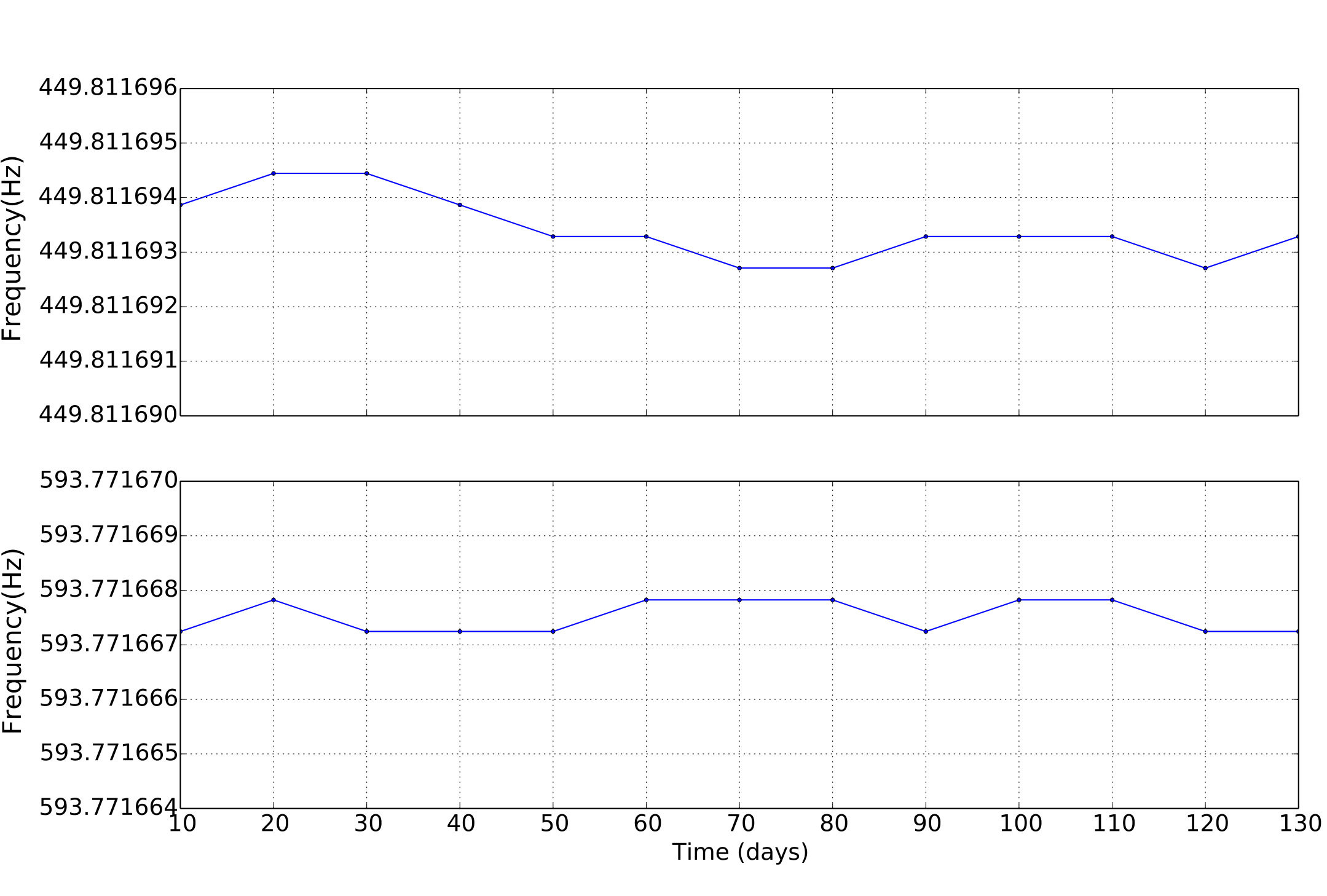 Figure 2
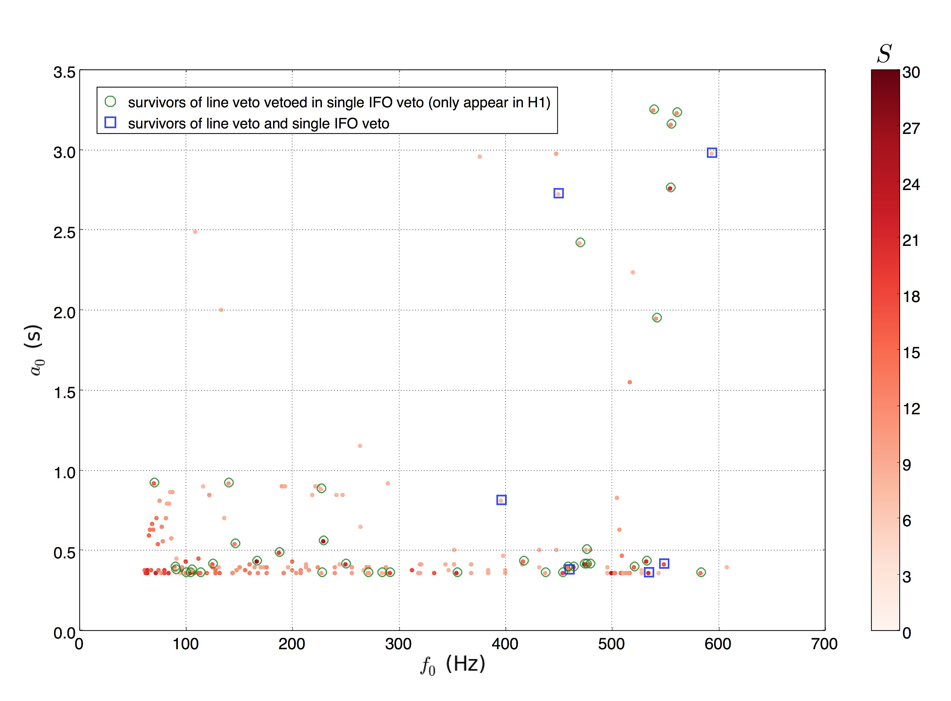 Figure 3
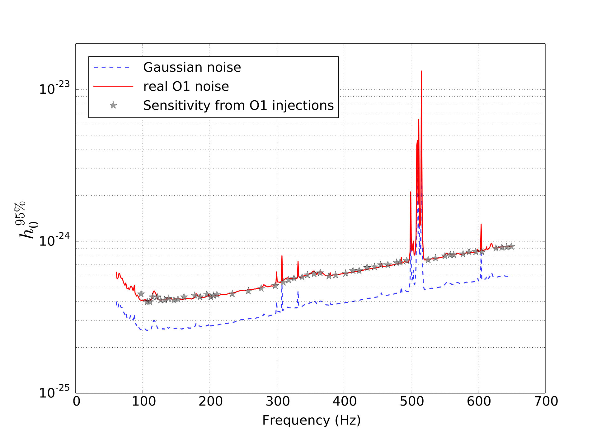 Figure 4
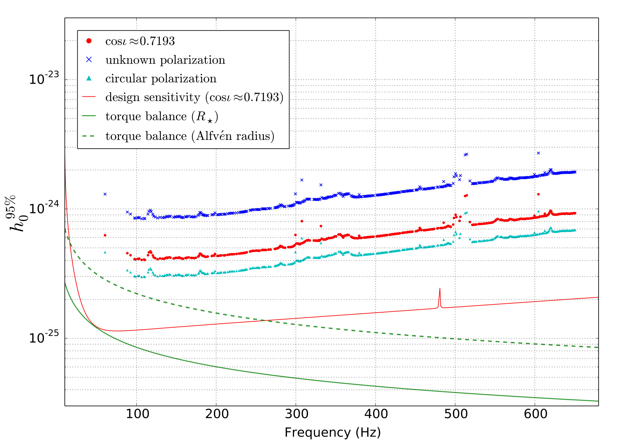 Figure 5
| Observed parameter | Symbol | Value | Reference |
| Right ascension | 16h 19m 55.0850s | Bradshaw et al. (1999) | |
| Declination | Bradshaw et al. (1999) | ||
| X-ray flux | Watts et al. (2008) | ||
| Orbital period | s | Galloway et al. (2014) | |
| Projected semi-major axis | s | Steeghs et al. (2002) | |
| Polarization angle | Fomalont et al. (2001) | ||
| Inclination angle | Fomalont et al. (2001) | ||
| Search parameter | Symbol | Search range | Resolution |
| Frequency | Hz | Hz | |
| Projected semi-major axis | s | 0.01805 s |
| Veto | Number |
|---|---|
| First pass | 180 |
| After line veto | 44 |
| After single IFO veto | 6 |
| After half veto | 2 |
| After longer veto | 0 |
| Category | Score in one detector | Estimated frequency in one detector | Action |
|---|---|---|---|
| A | in one detector but in the other | where | Veto |
| B | in one detector but in the other | where | Keep |
| C | in both detectors | Keep | |
| D | in both detectors | Keep |
| Sub-band (Hz) | (Hz) | (s) | ||||
|---|---|---|---|---|---|---|
| () | ||||||
| 395–396 | 395.8561536 | 3 | 0.81 | 8.05153 | 6.55545 | 9.13679 |
| 449–450* | 449.8116935 | 3 | 2.73 | 7.38701 | 6.46122 | 6.50190 |
| 459–460 | 459.5557459 | 6 | 0.38 | 12.76130 | 14.61070 | 6.30887 |
| 534–535 | 534.3625717 | 4 | 0.36 | 20.18630 | 20.53770 | 6.97788 |
| 548–549 | 548.9457104 | 7 | 0.42 | 16.68650 | 18.39020 | 6.46258 |
| 593–594* | 593.7716675 | 1 | 2.98 | 7.40397 | 6.17976 | 5.88553 |
| Higher with longer | Lower with longer | |
|---|---|---|
| Low spin wandering | Follow up with more sensitive method | Veto |
| High spin wandering | Unlikely to happen | Follow up with more sensitive method |
| guided by observed Viterbi path |
| Quantity | 449–450 Hz | 593–594 Hz | |
|---|---|---|---|
| 10 d | 7.38701 | 7.40397 | |
| (Hz) | 449.8116936 | 593.7716675 | |
| (s) | 2.73 | 2.98 | |
| 20 d | 6.93366 | 6.93900 | |
| (Hz) | 449.7891863 | 593.6174193 | |
| (s) | 1.70 | 1.79 |
| Data | (Hz) | (s) | () | |||||||
|---|---|---|---|---|---|---|---|---|---|---|
| S5 | 64.5774908 | 0.81 | 9.58 | 9.12097 | 7.42935* | 7.67254 | 11.7985 | |||
| S5 | 102.2907797 | 2.47 | 9.81 | 20.81940 | 16.17190 | 12.00540 | 20.63850 | 17.38740 | 25.81390 | |
| S5 | 202.8863982 | 2.34 | 11.25 | 15.80950 | 18.54850 | 17.46390 | 19.15680 | 18.9102 | 21.4415 | |
| S5 | 254.6697757 | 3.03 | 14.55 | 0.0375 | 12.50180 | 9.27111 | 10.8953 | 7.74954 | 15.0849 | |
| O1 | 97.2345635 | 2.15 | 4.50 | 0.71935 | 9.76216 | 7.53014* | 7.29089 | 8.91108 | 9.98727 | |
| O1 | 132.1234568 | 0.70 | 4.80 | 16.86500 | 8.90286 | 8.63928 | 13.29010 | 13.30940 | 19.54900 | |
| O1 | 185.8094752 | 1.11 | 9.90 | 0.37952 | 19.05450 | 14.44080 | 12.70840 | 18.07160 | 17.95120 | 20.34430 |
| O1 | 233.9125689 | 0.46 | 4.60 | 0.70917 | 16.71220 | 9.18889 | 12.25070 | 13.15180 | 18.02530 | |
| O1 | 345.3456700 | 1.45 | 7.00 | 0.71567 | 14.09400 | 9.15852 | 10.10120 | 12.83390 | 14.72410 | |
| O1 | 454.4563891 | 3.20 | 7.00 | 9.03162 | 7.54074* | 9.06928 | ||||
| O1 | 525.7096896 | 2.81 | 12.90 | 0.66578 | 11.55910 | 7.83362 | 8.90156 | 11.35370 | 10.04660 | 13.26430 |
| O1 | 635.6679700 | 1.98 | 10.00 | 0.72650 | 10.64010 | 8.91769 | 9.13239 | 11.56240 |
Peer Reviews
No public reviews on file for this paper yet. If you reviewed it on a platform where reviews are public (OpenReview, ICLR, NeurIPS, ICML), you can paste yours below so the community can read it here.
Videos
No videos yet. Explain this paper in a talk, walkthrough, or lecture? Add one.
Search for gravitational waves from Scorpius X-1 in the first Advanced LIGO observing run with a hidden Markov model
B. P. Abbott,1 R. Abbott,1 T. D. Abbott,2 F. Acernese,3,4 K. Ackley,5 C. Adams,6 T. Adams,7 P. Addesso,8 R. X. Adhikari,1 V. B. Adya,9 C. Affeldt,9 M. Afrough,10 B. Agarwal,11 K. Agatsuma,12 N. Aggarwal,13 O. D. Aguiar,14 L. Aiello,15,16 A. Ain,17 P. Ajith,18 B. Allen,9,19,20 G. Allen,11 A. Allocca,21,22 H. Almoubayyed,23 P. A. Altin,24 A. Amato,25 A. Ananyeva,1 S. B. Anderson,1 W. G. Anderson,19 S. Antier,26 S. Appert,1 K. Arai,1 M. C. Araya,1 J. S. Areeda,27 N. Arnaud,26,28 K. G. Arun,29 S. Ascenzi,30,16 G. Ashton,9 M. Ast,31 S. M. Aston,6 P. Astone,32 P. Aufmuth,20 C. Aulbert,9 K. AultONeal,33 A. Avila-Alvarez,27 S. Babak,34 P. Bacon,35 M. K. M. Bader,12 S. Bae,36 P. T. Baker,37,38 F. Baldaccini,39,40 G. Ballardin,28 S. W. Ballmer,41 S. Banagiri,42 J. C. Barayoga,1 S. E. Barclay,23 B. C. Barish,1 D. Barker,43 F. Barone,3,4 B. Barr,23 L. Barsotti,13 M. Barsuglia,35 D. Barta,44 J. Bartlett,43 I. Bartos,45 R. Bassiri,46 A. Basti,21,22 J. C. Batch,43 C. Baune,9 M. Bawaj,47,40 M. Bazzan,48,49 B. Bécsy,50 C. Beer,9 M. Bejger,51 I. Belahcene,26 A. S. Bell,23 B. K. Berger,1 G. Bergmann,9 C. P. L. Berry,52 D. Bersanetti,53,54 A. Bertolini,12 Z. B.Etienne,37,38 J. Betzwieser,6 S. Bhagwat,41 R. Bhandare,55 I. A. Bilenko,56 G. Billingsley,1 C. R. Billman,5 J. Birch,6 R. Birney,57 O. Birnholtz,9 S. Biscans,13 A. Bisht,20 M. Bitossi,28,22 C. Biwer,41 M. A. Bizouard,26 J. K. Blackburn,1 J. Blackman,58 C. D. Blair,59 D. G. Blair,59 R. M. Blair,43 S. Bloemen,60 O. Bock,9 N. Bode,9 M. Boer,61 G. Bogaert,61 A. Bohe,34 F. Bondu,62 R. Bonnand,7 B. A. Boom,12 R. Bork,1 V. Boschi,21,22 S. Bose,63,17 Y. Bouffanais,35 A. Bozzi,28 C. Bradaschia,22 P. R. Brady,19 V. B. Braginsky∗,56 M. Branchesi,64,65 J. E. Brau,66 T. Briant,67 A. Brillet,61 M. Brinkmann,9 V. Brisson,26 P. Brockill,19 J. E. Broida,68 A. F. Brooks,1 D. A. Brown,41 D. D. Brown,52 N. M. Brown,13 S. Brunett,1 C. C. Buchanan,2 A. Buikema,13 T. Bulik,69 H. J. Bulten,70,12 A. Buonanno,34,71 D. Buskulic,7 C. Buy,35 R. L. Byer,46 M. Cabero,9 L. Cadonati,72 G. Cagnoli,25,73 C. Cahillane,1 J. Calderón Bustillo,72 T. A. Callister,1 E. Calloni,74,4 J. B. Camp,75 M. Canepa,53,54 P. Canizares,60 K. C. Cannon,76 H. Cao,77 J. Cao,78 C. D. Capano,9 E. Capocasa,35 F. Carbognani,28 S. Caride,79 M. F. Carney,80 J. Casanueva Diaz,26 C. Casentini,30,16 S. Caudill,19 M. Cavaglià,10 F. Cavalier,26 R. Cavalieri,28 G. Cella,22 C. B. Cepeda,1 L. Cerboni Baiardi,64,65 G. Cerretani,21,22 E. Cesarini,30,16 S. J. Chamberlin,81 M. Chan,23 S. Chao,82 P. Charlton,83 E. Chassande-Mottin,35 D. Chatterjee,19 B. D. Cheeseboro,37,38 H. Y. Chen,84 Y. Chen,58 H.-P. Cheng,5 A. Chincarini,54 A. Chiummo,28 T. Chmiel,80 H. S. Cho,85 M. Cho,71 J. H. Chow,24 N. Christensen,68,61 Q. Chu,59 A. J. K. Chua,86 S. Chua,67 A. K. W. Chung,87 S. Chung,59 G. Ciani,5 R. Ciolfi,88,89 C. E. Cirelli,46 A. Cirone,53,54 F. Clara,43 J. A. Clark,72 F. Cleva,61 C. Cocchieri,10 E. Coccia,15,16 P.-F. Cohadon,67 A. Colla,90,32 C. G. Collette,91 L. R. Cominsky,92 M. Constancio Jr.,14 L. Conti,49 S. J. Cooper,52 P. Corban,6 T. R. Corbitt,2 K. R. Corley,45 N. Cornish,93 A. Corsi,79 S. Cortese,28 C. A. Costa,14 M. W. Coughlin,68 S. B. Coughlin,94,95 J.-P. Coulon,61 S. T. Countryman,45 P. Couvares,1 P. B. Covas,96 E. E. Cowan,72 D. M. Coward,59 M. J. Cowart,6 D. C. Coyne,1 R. Coyne,79 J. D. E. Creighton,19 T. D. Creighton,97 J. Cripe,2 S. G. Crowder,98 T. J. Cullen,27 A. Cumming,23 L. Cunningham,23 E. Cuoco,28 T. Dal Canton,75 S. L. Danilishin,20,9 S. D’Antonio,16 K. Danzmann,20,9 A. Dasgupta,99 C. F. Da Silva Costa,5 V. Dattilo,28 I. Dave,55 M. Davier,26 G. S. Davies,23 D. Davis,41 E. J. Daw,100 B. Day,72 S. De,41 D. DeBra,46 E. Deelman,101 J. Degallaix,25 M. De Laurentis,74,4 S. Deléglise,67 W. Del Pozzo,52,21,22 T. Denker,9 T. Dent,9 V. Dergachev,34 R. De Rosa,74,4 R. T. DeRosa,6 R. DeSalvo,102 J. Devenson,57 R. C. Devine,37,38 S. Dhurandhar,17 M. C. Díaz,97 L. Di Fiore,4 M. Di Giovanni,103,89 T. Di Girolamo,74,4,45 A. Di Lieto,21,22 S. Di Pace,90,32 I. Di Palma,90,32 F. Di Renzo,21,22 Z. Doctor,84 V. Dolique,25 F. Donovan,13 K. L. Dooley,10 S. Doravari,9 I. Dorrington,95 R. Douglas,23 M. Dovale Álvarez,52 T. P. Downes,19 M. Drago,9 R. W. P. Drever*♯,1 J. C. Driggers,43 Z. Du,78 M. Ducrot,7 J. Duncan,94 S. E. Dwyer,43 T. B. Edo,100 M. C. Edwards,68 A. Effler,6 H.-B. Eggenstein,9 P. Ehrens,1 J. Eichholz,1 S. S. Eikenberry,5 R. C. Essick,13 T. Etzel,1 M. Evans,13 T. M. Evans,6 M. Factourovich,45 V. Fafone,30,16,15 H. Fair,41 S. Fairhurst,95 X. Fan,78 S. Farinon,54 B. Farr,84 W. M. Farr,52 E. J. Fauchon-Jones,95 M. Favata,104 M. Fays,95 H. Fehrmann,9 J. Feicht,1 M. M. Fejer,46 A. Fernandez-Galiana,13 I. Ferrante,21,22 E. C. Ferreira,14 F. Ferrini,28 F. Fidecaro,21,22 I. Fiori,28 D. Fiorucci,35 R. P. Fisher,41 R. Flaminio,25,105 M. Fletcher,23 H. Fong,106 P. W. F. Forsyth,24 S. S. Forsyth,72 J.-D. Fournier,61 S. Frasca,90,32 F. Frasconi,22 Z. Frei,50 A. Freise,52 R. Frey,66 V. Frey,26 E. M. Fries,1 P. Fritschel,13 V. V. Frolov,6 P. Fulda,5,75 M. Fyffe,6 H. Gabbard,9 M. Gabel,107 B. U. Gadre,17 S. M. Gaebel,52 J. R. Gair,108 L. Gammaitoni,39 M. R. Ganija,77 S. G. Gaonkar,17 F. Garufi,74,4 S. Gaudio,33 G. Gaur,109 V. Gayathri,110 N. Gehrels†,75 G. Gemme,54 E. Genin,28 A. Gennai,22 D. George,11 J. George,55 L. Gergely,111 V. Germain,7 S. Ghonge,72 Abhirup Ghosh,18 Archisman Ghosh,18,12 S. Ghosh,60,12 J. A. Giaime,2,6 K. D. Giardina,6 A. Giazotto,22 K. Gill,33 L. Glover,102 E. Goetz,9 R. Goetz,5 S. Gomes,95 G. González,2 J. M. Gonzalez Castro,21,22 A. Gopakumar,112 M. L. Gorodetsky,56 S. E. Gossan,1 M. Gosselin,28 R. Gouaty,7 A. Grado,113,4 C. Graef,23 M. Granata,25 A. Grant,23 S. Gras,13 C. Gray,43 G. Greco,64,65 A. C. Green,52 P. Groot,60 H. Grote,9 S. Grunewald,34 P. Gruning,26 G. M. Guidi,64,65 X. Guo,78 A. Gupta,81 M. K. Gupta,99 K. E. Gushwa,1 E. K. Gustafson,1 R. Gustafson,114 B. R. Hall,63 E. D. Hall,1 G. Hammond,23 M. Haney,112 M. M. Hanke,9 J. Hanks,43 C. Hanna,81 O. A. Hannuksela,87 J. Hanson,6 T. Hardwick,2 J. Harms,64,65 G. M. Harry,115 I. W. Harry,34 M. J. Hart,23 C.-J. Haster,106 K. Haughian,23 J. Healy,116 A. Heidmann,67 M. C. Heintze,6 H. Heitmann,61 P. Hello,26 G. Hemming,28 M. Hendry,23 I. S. Heng,23 J. Hennig,23 J. Henry,116 A. W. Heptonstall,1 M. Heurs,9,20 S. Hild,23 D. Hoak,28 D. Hofman,25 K. Holt,6 D. E. Holz,84 P. Hopkins,95 C. Horst,19 J. Hough,23 E. A. Houston,23 E. J. Howell,59 Y. M. Hu,9 E. A. Huerta,11 D. Huet,26 B. Hughey,33 S. Husa,96 S. H. Huttner,23 T. Huynh-Dinh,6 N. Indik,9 D. R. Ingram,43 R. Inta,79 G. Intini,90,32 H. N. Isa,23 J.-M. Isac,67 M. Isi,1 B. R. Iyer,18 K. Izumi,43 T. Jacqmin,67 K. Jani,72 P. Jaranowski,117 S. Jawahar,118 F. Jiménez-Forteza,96 W. W. Johnson,2 D. I. Jones,119 R. Jones,23 R. J. G. Jonker,12 L. Ju,59 J. Junker,9 C. V. Kalaghatgi,95 V. Kalogera,94 S. Kandhasamy,6 G. Kang,36 J. B. Kanner,1 S. Karki,66 K. S. Karvinen,9 M. Kasprzack,2 M. Katolik,11 E. Katsavounidis,13 W. Katzman,6 S. Kaufer,20 K. Kawabe,43 F. Kéfélian,61 D. Keitel,23 A. J. Kemball,11 R. Kennedy,100 C. Kent,95 J. S. Key,120 F. Y. Khalili,56 I. Khan,15,16 S. Khan,9 Z. Khan,99 E. A. Khazanov,121 N. Kijbunchoo,43 Chunglee Kim,122 J. C. Kim,123 W. Kim,77 W. S. Kim,124 Y.-M. Kim,85,122 S. J. Kimbrell,72 E. J. King,77 P. J. King,43 R. Kirchhoff,9 J. S. Kissel,43 L. Kleybolte,31 S. Klimenko,5 P. Koch,9 S. M. Koehlenbeck,9 S. Koley,12 V. Kondrashov,1 A. Kontos,13 M. Korobko,31 W. Z. Korth,1 I. Kowalska,69 D. B. Kozak,1 C. Krämer,9 V. Kringel,9 B. Krishnan,9 A. Królak,125,126 G. Kuehn,9 P. Kumar,106 R. Kumar,99 S. Kumar,18 L. Kuo,82 A. Kutynia,125 S. Kwang,19 B. D. Lackey,34 K. H. Lai,87 M. Landry,43 R. N. Lang,19 J. Lange,116 B. Lantz,46 R. K. Lanza,13 A. Lartaux-Vollard,26 P. D. Lasky,127 M. Laxen,6 A. Lazzarini,1 C. Lazzaro,49 P. Leaci,90,32 S. Leavey,23 C. H. Lee,85 H. K. Lee,128 H. M. Lee,122 H. W. Lee,123 K. Lee,23 J. Lehmann,9 A. Lenon,37,38 M. Leonardi,103,89 N. Leroy,26 N. Letendre,7 Y. Levin,127 T. G. F. Li,87 A. Libson,13 T. B. Littenberg,129 J. Liu,59 N. A. Lockerbie,118 L. T. London,95 J. E. Lord,41 M. Lorenzini,15,16 V. Loriette,130 M. Lormand,6 G. Losurdo,22 J. D. Lough,9,20 G. Lovelace,27 H. Lück,20,9 D. Lumaca,30,16 A. P. Lundgren,9 R. Lynch,13 Y. Ma,58 S. Macfoy,57 B. Machenschalk,9 M. MacInnis,13 D. M. Macleod,2 I. Magaña Hernandez,87 F. Magaña-Sandoval,41 L. Magaña Zertuche,41 R. M. Magee,81 E. Majorana,32 I. Maksimovic,130 N. Man,61 V. Mandic,42 V. Mangano,23 G. L. Mansell,24 M. Manske,19 M. Mantovani,28 F. Marchesoni,47,40 F. Marion,7 S. Márka,45 Z. Márka,45 C. Markakis,11 A. S. Markosyan,46 E. Maros,1 F. Martelli,64,65 L. Martellini,61 I. W. Martin,23 D. V. Martynov,13 J. N. Marx,1 K. Mason,13 A. Masserot,7 T. J. Massinger,1 M. Masso-Reid,23 S. Mastrogiovanni,90,32 A. Matas,42 F. Matichard,13 L. Matone,45 N. Mavalvala,13 R. Mayani,101 N. Mazumder,63 R. McCarthy,43 D. E. McClelland,24 S. McCormick,6 L. McCuller,13 S. C. McGuire,131 G. McIntyre,1 J. McIver,1 D. J. McManus,24 T. McRae,24 S. T. McWilliams,37,38 D. Meacher,81 G. D. Meadors,34,9 J. Meidam,12 E. Mejuto-Villa,8 A. Melatos,132 G. Mendell,43 R. A. Mercer,19 E. L. Merilh,43 M. Merzougui,61 S. Meshkov,1 C. Messenger,23 C. Messick,81 R. Metzdorff,67 P. M. Meyers,42 F. Mezzani,32,90 H. Miao,52 C. Michel,25 H. Middleton,52 E. E. Mikhailov,133 L. Milano,74,4 A. L. Miller,5 A. Miller,90,32 B. B. Miller,94 J. Miller,13 M. Millhouse,93 O. Minazzoli,61 Y. Minenkov,16 J. Ming,34 C. Mishra,134 S. Mitra,17 V. P. Mitrofanov,56 G. Mitselmakher,5 R. Mittleman,13 A. Moggi,22 M. Mohan,28 S. R. P. Mohapatra,13 M. Montani,64,65 B. C. Moore,104 C. J. Moore,86 D. Moraru,43 G. Moreno,43 S. R. Morriss,97 B. Mours,7 C. M. Mow-Lowry,52 G. Mueller,5 A. W. Muir,95 Arunava Mukherjee,9 D. Mukherjee,19 S. Mukherjee,97 N. Mukund,17 A. Mullavey,6 J. Munch,77 E. A. M. Muniz,41 P. G. Murray,23 K. Napier,72 I. Nardecchia,30,16 L. Naticchioni,90,32 R. K. Nayak,135 G. Nelemans,60,12 T. J. N. Nelson,6 M. Neri,53,54 M. Nery,9 A. Neunzert,114 J. M. Newport,115 G. Newton‡,23 K. K. Y. Ng,87 T. T. Nguyen,24 D. Nichols,60 A. B. Nielsen,9 S. Nissanke,60,12 A. Nitz,9 A. Noack,9 F. Nocera,28 D. Nolting,6 M. E. N. Normandin,97 L. K. Nuttall,41 J. Oberling,43 E. Ochsner,19 E. Oelker,13 G. H. Ogin,107 J. J. Oh,124 S. H. Oh,124 F. Ohme,9 M. Oliver,96 P. Oppermann,9 Richard J. Oram,6 B. O’Reilly,6 R. Ormiston,42 L. F. Ortega,5 R. O’Shaughnessy,116 D. J. Ottaway,77 H. Overmier,6 B. J. Owen,79 A. E. Pace,81 J. Page,129 M. A. Page,59 A. Pai,110 S. A. Pai,55 J. R. Palamos,66 O. Palashov,121 C. Palomba,32 A. Pal-Singh,31 H. Pan,82 B. Pang,58 P. T. H. Pang,87 C. Pankow,94 F. Pannarale,95 B. C. Pant,55 F. Paoletti,22 A. Paoli,28 M. A. Papa,34,19,9 H. R. Paris,46 W. Parker,6 D. Pascucci,23 A. Pasqualetti,28 R. Passaquieti,21,22 D. Passuello,22 B. Patricelli,136,22 B. L. Pearlstone,23 M. Pedraza,1 R. Pedurand,25,137 L. Pekowsky,41 A. Pele,6 S. Penn,138 C. J. Perez,43 A. Perreca,1,103,89 L. M. Perri,94 H. P. Pfeiffer,106 M. Phelps,23 O. J. Piccinni,90,32 M. Pichot,61 F. Piergiovanni,64,65 V. Pierro,8 G. Pillant,28 L. Pinard,25 I. M. Pinto,8 M. Pitkin,23 R. Poggiani,21,22 P. Popolizio,28 E. K. Porter,35 A. Post,9 J. Powell,23 J. Prasad,17 J. W. W. Pratt,33 V. Predoi,95 T. Prestegard,19 M. Prijatelj,9 M. Principe,8 S. Privitera,34 R. Prix,9 G. A. Prodi,103,89 L. G. Prokhorov,56 O. Puncken,9 M. Punturo,40 P. Puppo,32 M. Pürrer,34 H. Qi,19 J. Qin,59 S. Qiu,127 V. Quetschke,97 E. A. Quintero,1 R. Quitzow-James,66 F. J. Raab,43 D. S. Rabeling,24 H. Radkins,43 P. Raffai,50 S. Raja,55 C. Rajan,55 M. Rakhmanov,97 K. E. Ramirez,97 P. Rapagnani,90,32 V. Raymond,34 M. Razzano,21,22 J. Read,27 T. Regimbau,61 L. Rei,54 S. Reid,57 D. H. Reitze,1,5 H. Rew,133 S. D. Reyes,41 F. Ricci,90,32 P. M. Ricker,11 S. Rieger,9 K. Riles,114 M. Rizzo,116 N. A. Robertson,1,23 R. Robie,23 F. Robinet,26 A. Rocchi,16 L. Rolland,7 J. G. Rollins,1 V. J. Roma,66 R. Romano,3,4 C. L. Romel,43 J. H. Romie,6 D. Rosińska,139,51 M. P. Ross,140 S. Rowan,23 A. Rüdiger,9 P. Ruggi,28 K. Ryan,43 M. Rynge,101 S. Sachdev,1 T. Sadecki,43 L. Sadeghian,19 M. Sakellariadou,141 L. Salconi,28 M. Saleem,110 F. Salemi,9 A. Samajdar,135 L. Sammut,127 L. M. Sampson,94 E. J. Sanchez,1 V. Sandberg,43 B. Sandeen,94 J. R. Sanders,41 B. Sassolas,25 B. S. Sathyaprakash,81,95 P. R. Saulson,41 O. Sauter,114 R. L. Savage,43 A. Sawadsky,20 P. Schale,66 J. Scheuer,94 E. Schmidt,33 J. Schmidt,9 P. Schmidt,1,60 R. Schnabel,31 R. M. S. Schofield,66 A. Schönbeck,31 E. Schreiber,9 D. Schuette,9,20 B. W. Schulte,9 B. F. Schutz,95,9 S. G. Schwalbe,33 J. Scott,23 S. M. Scott,24 E. Seidel,11 D. Sellers,6 A. S. Sengupta,142 D. Sentenac,28 V. Sequino,30,16 A. Sergeev,121 D. A. Shaddock,24 T. J. Shaffer,43 A. A. Shah,129 M. S. Shahriar,94 L. Shao,34 B. Shapiro,46 P. Shawhan,71 A. Sheperd,19 D. H. Shoemaker,13 D. M. Shoemaker,72 K. Siellez,72 X. Siemens,19 M. Sieniawska,51 D. Sigg,43 A. D. Silva,14 A. Singer,1 L. P. Singer,75 A. Singh,34,9,20 R. Singh,2 A. Singhal,15,32 A. M. Sintes,96 B. J. J. Slagmolen,24 B. Smith,6 J. R. Smith,27 R. J. E. Smith,1 E. J. Son,124 J. A. Sonnenberg,19 B. Sorazu,23 F. Sorrentino,54 T. Souradeep,17 A. P. Spencer,23 A. K. Srivastava,99 A. Staley,45 M. Steinke,9 J. Steinlechner,23,31 S. Steinlechner,31 D. Steinmeyer,9,20 B. C. Stephens,19 R. Stone,97 K. A. Strain,23 G. Stratta,64,65 S. E. Strigin,56 R. Sturani,143 A. L. Stuver,6 T. Z. Summerscales,144 L. Sun,132 S. Sunil,99 P. J. Sutton,95 B. L. Swinkels,28 M. J. Szczepańczyk,33 M. Tacca,35 D. Talukder,66 D. B. Tanner,5 M. Tápai,111 A. Taracchini,34 J. A. Taylor,129 R. Taylor,1 T. Theeg,9 E. G. Thomas,52 M. Thomas,6 P. Thomas,43 K. A. Thorne,6 K. S. Thorne,58 E. Thrane,127 S. Tiwari,15,89 V. Tiwari,95 K. V. Tokmakov,118 K. Toland,23 M. Tonelli,21,22 Z. Tornasi,23 C. I. Torrie,1 D. Töyrä,52 F. Travasso,28,40 G. Traylor,6 D. Trifirò,10 J. Trinastic,5 M. C. Tringali,103,89 L. Trozzo,145,22 K. W. Tsang,12 M. Tse,13 R. Tso,1 D. Tuyenbayev,97 K. Ueno,19 D. Ugolini,146 C. S. Unnikrishnan,112 A. L. Urban,1 S. A. Usman,95 K. Vahi,101 H. Vahlbruch,20 G. Vajente,1 G. Valdes,97 N. van Bakel,12 M. van Beuzekom,12 J. F. J. van den Brand,70,12 C. Van Den Broeck,12 D. C. Vander-Hyde,41 L. van der Schaaf,12 J. V. van Heijningen,12 A. A. van Veggel,23 M. Vardaro,48,49 V. Varma,58 S. Vass,1 M. Vasúth,44 A. Vecchio,52 G. Vedovato,49 J. Veitch,52 P. J. Veitch,77 K. Venkateswara,140 G. Venugopalan,1 D. Verkindt,7 F. Vetrano,64,65 A. Viceré,64,65 A. D. Viets,19 S. Vinciguerra,52 D. J. Vine,57 J.-Y. Vinet,61 S. Vitale,13 T. Vo,41 H. Vocca,39,40 C. Vorvick,43 D. V. Voss,5 W. D. Vousden,52 S. P. Vyatchanin,56 A. R. Wade,1 L. E. Wade,80 M. Wade,80 R. Walet,12 M. Walker,2 L. Wallace,1 S. Walsh,19 G. Wang,15,65 H. Wang,52 J. Z. Wang,81 M. Wang,52 Y.-F. Wang,87 Y. Wang,59 R. L. Ward,24 J. Warner,43 M. Was,7 J. Watchi,91 B. Weaver,43 L.-W. Wei,9,20 M. Weinert,9 A. J. Weinstein,1 R. Weiss,13 L. Wen,59 E. K. Wessel,11 P. Weßels,9 T. Westphal,9 K. Wette,9 J. T. Whelan,116 B. F. Whiting,5 C. Whittle,127 D. Williams,23 R. D. Williams,1 A. R. Williamson,116 J. L. Willis,147 B. Willke,20,9 M. H. Wimmer,9,20 W. Winkler,9 C. C. Wipf,1 H. Wittel,9,20 G. Woan,23 J. Woehler,9 J. Wofford,116 K. W. K. Wong,87 J. Worden,43 J. L. Wright,23 D. S. Wu,9 G. Wu,6 W. Yam,13 H. Yamamoto,1 C. C. Yancey,71 M. J. Yap,24 Hang Yu,13 Haocun Yu,13 M. Yvert,7 A. Zadrożny,125 M. Zanolin,33 T. Zelenova,28 J.-P. Zendri,49 M. Zevin,94 L. Zhang,1 M. Zhang,133 T. Zhang,23 Y.-H. Zhang,116 C. Zhao,59 M. Zhou,94 Z. Zhou,94 X. J. Zhu,59 M. E. Zucker,1,13 and J. Zweizig1*
(LIGO Scientific Collaboration and Virgo Collaboration)
*∗*Deceased, March 2016. *♯*Deceased, March 2017. *†*Deceased, February 2017. *‡*Deceased, December 2016.
S. Suvorova,132,148 W. Moran,148 and R. J. Evans132
LIGO, California Institute of Technology, Pasadena, CA 91125, USA
Louisiana State University, Baton Rouge, LA 70803, USA
Università di Salerno, Fisciano, I-84084 Salerno, Italy
INFN, Sezione di Napoli, Complesso Universitario di Monte S.Angelo, I-80126 Napoli, Italy
University of Florida, Gainesville, FL 32611, USA
LIGO Livingston Observatory, Livingston, LA 70754, USA
Laboratoire d’Annecy-le-Vieux de Physique des Particules (LAPP), Université Savoie Mont Blanc, CNRS/IN2P3, F-74941 Annecy, France
University of Sannio at Benevento, I-82100 Benevento, Italy and INFN, Sezione di Napoli, I-80100 Napoli, Italy
Albert-Einstein-Institut, Max-Planck-Institut für Gravitationsphysik, D-30167 Hannover, Germany
The University of Mississippi, University, MS 38677, USA
NCSA, University of Illinois at Urbana-Champaign, Urbana, IL 61801, USA
Nikhef, Science Park, 1098 XG Amsterdam, The Netherlands
LIGO, Massachusetts Institute of Technology, Cambridge, MA 02139, USA
Instituto Nacional de Pesquisas Espaciais, 12227-010 São José dos Campos, São Paulo, Brazil
Gran Sasso Science Institute (GSSI), I-67100 L’Aquila, Italy
INFN, Sezione di Roma Tor Vergata, I-00133 Roma, Italy
Inter-University Centre for Astronomy and Astrophysics, Pune 411007, India
International Centre for Theoretical Sciences, Tata Institute of Fundamental Research, Bengaluru 560089, India
University of Wisconsin-Milwaukee, Milwaukee, WI 53201, USA
Leibniz Universität Hannover, D-30167 Hannover, Germany
Università di Pisa, I-56127 Pisa, Italy
INFN, Sezione di Pisa, I-56127 Pisa, Italy
SUPA, University of Glasgow, Glasgow G12 8QQ, United Kingdom
Australian National University, Canberra, Australian Capital Territory 0200, Australia
Laboratoire des Matériaux Avancés (LMA), CNRS/IN2P3, F-69622 Villeurbanne, France
LAL, Univ. Paris-Sud, CNRS/IN2P3, Université Paris-Saclay, F-91898 Orsay, France
California State University Fullerton, Fullerton, CA 92831, USA
European Gravitational Observatory (EGO), I-56021 Cascina, Pisa, Italy
Chennai Mathematical Institute, Chennai 603103, India
Università di Roma Tor Vergata, I-00133 Roma, Italy
Universität Hamburg, D-22761 Hamburg, Germany
INFN, Sezione di Roma, I-00185 Roma, Italy
Embry-Riddle Aeronautical University, Prescott, AZ 86301, USA
Albert-Einstein-Institut, Max-Planck-Institut für Gravitationsphysik, D-14476 Potsdam-Golm, Germany
APC, AstroParticule et Cosmologie, Université Paris Diderot, CNRS/IN2P3, CEA/Irfu, Observatoire de Paris, Sorbonne Paris Cité, F-75205 Paris Cedex 13, France
Korea Institute of Science and Technology Information, Daejeon 34141, Korea
West Virginia University, Morgantown, WV 26506, USA
Center for Gravitational Waves and Cosmology, West Virginia University, Morgantown, WV 26505, USA
Università di Perugia, I-06123 Perugia, Italy
INFN, Sezione di Perugia, I-06123 Perugia, Italy
Syracuse University, Syracuse, NY 13244, USA
University of Minnesota, Minneapolis, MN 55455, USA
LIGO Hanford Observatory, Richland, WA 99352, USA
Wigner RCP, RMKI, H-1121 Budapest, Konkoly Thege Miklós út 29-33, Hungary
Columbia University, New York, NY 10027, USA
Stanford University, Stanford, CA 94305, USA
Università di Camerino, Dipartimento di Fisica, I-62032 Camerino, Italy
Università di Padova, Dipartimento di Fisica e Astronomia, I-35131 Padova, Italy
INFN, Sezione di Padova, I-35131 Padova, Italy
MTA Eötvös University, “Lendulet” Astrophysics Research Group, Budapest 1117, Hungary
Nicolaus Copernicus Astronomical Center, Polish Academy of Sciences, 00-716, Warsaw, Poland
University of Birmingham, Birmingham B15 2TT, United Kingdom
Università degli Studi di Genova, I-16146 Genova, Italy
INFN, Sezione di Genova, I-16146 Genova, Italy
RRCAT, Indore MP 452013, India
Faculty of Physics, Lomonosov Moscow State University, Moscow 119991, Russia
SUPA, University of the West of Scotland, Paisley PA1 2BE, United Kingdom
Caltech CaRT, Pasadena, CA 91125, USA
University of Western Australia, Crawley, Western Australia 6009, Australia
Department of Astrophysics/IMAPP, Radboud University Nijmegen, P.O. Box 9010, 6500 GL Nijmegen, The Netherlands
Artemis, Université Côte d’Azur, Observatoire Côte d’Azur, CNRS, CS 34229, F-06304 Nice Cedex 4, France
Institut de Physique de Rennes, CNRS, Université de Rennes 1, F-35042 Rennes, France
Washington State University, Pullman, WA 99164, USA
Università degli Studi di Urbino ’Carlo Bo’, I-61029 Urbino, Italy
INFN, Sezione di Firenze, I-50019 Sesto Fiorentino, Firenze, Italy
University of Oregon, Eugene, OR 97403, USA
Laboratoire Kastler Brossel, UPMC-Sorbonne Universités, CNRS, ENS-PSL Research University, Collège de France, F-75005 Paris, France
Carleton College, Northfield, MN 55057, USA
Astronomical Observatory Warsaw University, 00-478 Warsaw, Poland
VU University Amsterdam, 1081 HV Amsterdam, The Netherlands
University of Maryland, College Park, MD 20742, USA
Center for Relativistic Astrophysics and School of Physics, Georgia Institute of Technology, Atlanta, GA 30332, USA
Université Claude Bernard Lyon 1, F-69622 Villeurbanne, France
Università di Napoli ’Federico II’, Complesso Universitario di Monte S.Angelo, I-80126 Napoli, Italy
NASA Goddard Space Flight Center, Greenbelt, MD 20771, USA
RESCEU, University of Tokyo, Tokyo, 113-0033, Japan.
University of Adelaide, Adelaide, South Australia 5005, Australia
Tsinghua University, Beijing 100084, China
Texas Tech University, Lubbock, TX 79409, USA
Kenyon College, Gambier, OH 43022, USA
The Pennsylvania State University, University Park, PA 16802, USA
National Tsing Hua University, Hsinchu City, 30013 Taiwan, Republic of China
Charles Sturt University, Wagga Wagga, New South Wales 2678, Australia
University of Chicago, Chicago, IL 60637, USA
Pusan National University, Busan 46241, Korea
University of Cambridge, Cambridge CB2 1TN, United Kingdom
The Chinese University of Hong Kong, Shatin, NT, Hong Kong
INAF, Osservatorio Astronomico di Padova, Vicolo dell’Osservatorio 5, I-35122 Padova, Italy
INFN, Trento Institute for Fundamental Physics and Applications, I-38123 Povo, Trento, Italy
Università di Roma ’La Sapienza’, I-00185 Roma, Italy
Université Libre de Bruxelles, Brussels 1050, Belgium
Sonoma State University, Rohnert Park, CA 94928, USA
Montana State University, Bozeman, MT 59717, USA
Center for Interdisciplinary Exploration & Research in Astrophysics (CIERA), Northwestern University, Evanston, IL 60208, USA
Cardiff University, Cardiff CF24 3AA, United Kingdom
Universitat de les Illes Balears, IAC3—IEEC, E-07122 Palma de Mallorca, Spain
The University of Texas Rio Grande Valley, Brownsville, TX 78520, USA
Bellevue College, Bellevue, WA 98007, USA
Institute for Plasma Research, Bhat, Gandhinagar 382428, India
The University of Sheffield, Sheffield S10 2TN, United Kingdom
University of Southern California Information Sciences Institute, Marina Del Rey, CA 90292, USA
California State University, Los Angeles, 5151 State University Dr, Los Angeles, CA 90032, USA
Università di Trento, Dipartimento di Fisica, I-38123 Povo, Trento, Italy
Montclair State University, Montclair, NJ 07043, USA
National Astronomical Observatory of Japan, 2-21-1 Osawa, Mitaka, Tokyo 181-8588, Japan
Canadian Institute for Theoretical Astrophysics, University of Toronto, Toronto, Ontario M5S 3H8, Canada
Whitman College, 345 Boyer Avenue, Walla Walla, WA 99362 USA
School of Mathematics, University of Edinburgh, Edinburgh EH9 3FD, United Kingdom
University and Institute of Advanced Research, Gandhinagar Gujarat 382007, India
IISER-TVM, CET Campus, Trivandrum Kerala 695016, India
University of Szeged, Dóm tér 9, Szeged 6720, Hungary
Tata Institute of Fundamental Research, Mumbai 400005, India
INAF, Osservatorio Astronomico di Capodimonte, I-80131, Napoli, Italy
University of Michigan, Ann Arbor, MI 48109, USA
American University, Washington, D.C. 20016, USA
Rochester Institute of Technology, Rochester, NY 14623, USA
University of Białystok, 15-424 Białystok, Poland
SUPA, University of Strathclyde, Glasgow G1 1XQ, United Kingdom
University of Southampton, Southampton SO17 1BJ, United Kingdom
University of Washington Bothell, 18115 Campus Way NE, Bothell, WA 98011, USA
Institute of Applied Physics, Nizhny Novgorod, 603950, Russia
Seoul National University, Seoul 08826, Korea
Inje University Gimhae, South Gyeongsang 50834, Korea
National Institute for Mathematical Sciences, Daejeon 34047, Korea
NCBJ, 05-400 Świerk-Otwock, Poland
Institute of Mathematics, Polish Academy of Sciences, 00656 Warsaw, Poland
The School of Physics & Astronomy, Monash University, Clayton 3800, Victoria, Australia
Hanyang University, Seoul 04763, Korea
NASA Marshall Space Flight Center, Huntsville, AL 35811, USA
ESPCI, CNRS, F-75005 Paris, France
Southern University and A&M College, Baton Rouge, LA 70813, USA
The University of Melbourne, Parkville, Victoria 3010, Australia
College of William and Mary, Williamsburg, VA 23187, USA
Indian Institute of Technology Madras, Chennai 600036, India
IISER-Kolkata, Mohanpur, West Bengal 741252, India
Scuola Normale Superiore, Piazza dei Cavalieri 7, I-56126 Pisa, Italy
Université de Lyon, F-69361 Lyon, France
Hobart and William Smith Colleges, Geneva, NY 14456, USA
Janusz Gil Institute of Astronomy, University of Zielona Góra, 65-265 Zielona Góra, Poland
University of Washington, Seattle, WA 98195, USA
King’s College London, University of London, London WC2R 2LS, United Kingdom
Indian Institute of Technology, Gandhinagar Ahmedabad Gujarat 382424, India
International Institute of Physics, Universidade Federal do Rio Grande do Norte, Natal RN 59078-970, Brazil
Andrews University, Berrien Springs, MI 49104, USA
Università di Siena, I-53100 Siena, Italy
Trinity University, San Antonio, TX 78212, USA
Abilene Christian University, Abilene, TX 79699, USA
RMIT University, Melbourne, Victoria 3000, Australia
Abstract
Results are presented from a semi-coherent search for continuous gravitational waves from the brightest low-mass X-ray binary, Scorpius X-1, using data collected during the first Advanced LIGO observing run (O1). The search combines a frequency domain matched filter (Bessel-weighted -statistic) with a hidden Markov model to track wandering of the neutron star spin frequency. No evidence of gravitational waves is found in the frequency range 60–650 Hz. Frequentist 95% confidence strain upper limits, , , and for electromagnetically restricted source orientation, unknown polarization, and circular polarization, respectively, are reported at 106 Hz. They are times higher than the theoretical torque-balance limit at 106 Hz.
PACS numbers
95.85.Sz, 97.60.Jd
pacs:
Valid PACS appear here
††preprint: APS/123-QED
I Introduction
Rotating neutron stars are a possible source of persistent, periodic gravitational radiation. The signal is expected at specific multiples of the neutron star spin frequency Riles (2013). Astrophysical models suggest that the radiation may be emitted at levels detectable by ground-based, long-baseline interferometers such as the Laser Interferometer Gravitational Wave Observatory (LIGO) and the Virgo detector Harry et al. (2010); Aasi et al. (2015a); Acernese et al. (2015); Andersson et al. (2011); Riles (2013). A time-varying quadrupole moment can result from thermal Ushomirsky et al. (2000); Johnson-McDaniel and Owen (2013) or magnetic Cutler (2002); Mastrano et al. (2011); Lasky and Melatos (2013) gradients, r-modes Owen et al. (1998); Heyl (2002); Arras et al. (2003); Bondarescu et al. (2009), or nonaxisymmetric circulation in the superfluid interior Peralta et al. (2006); van Eysden and Melatos (2008); Bennett et al. (2010); Melatos et al. (2015).
Accreting neutron stars in binary systems are important search targets, because mass transfer spins up the star to Hz and may simultaneously drive several quadrupole-generating mechanisms Bildsten (1998); Andersson et al. (1999); Nayyar and Owen (2006); Melatos (2007); Vigelius and Melatos (2009). Moreover it is observed that the distribution of spin frequencies of low-mass X-ray binaries (LMXBs) cuts off near 620 Hz Chakrabarty et al. (2003), below the theoretical centrifugal break-up limit kHz Cook et al. (1994). This has been explained by hypothesizing that the gravitational radiation-reaction torque balances the accretion torque Papaloizou and Pringle (1978); Wagoner (1984); Bildsten (1998), implying a relation between the X-ray flux and gravitational wave strain. Scorpius X-1 (Sco X-1), the most X-ray-luminous LMXB, is therefore a promising target for gravitational wave searches.
Initial LIGO achieved its design sensitivity over a wide band during LIGO Science Run 5 (S5) Abbott et al. (2009) and exceeded it during Science Run 6 (S6) The LIGO Scientific Collaboration and The Virgo Collaboration (2012). The strain sensitivity of the next-generation Advanced LIGO interferometer is expected to improve ten-fold relative to Initial LIGO after several stages of upgrade Harry and the LIGO Scientific Collaboration (2010). In the first observation run (O1), from September 2015 to January 2016, the strain noise is three to four times lower than in S6 across the most sensitive band, between 100 Hz and 300 Hz, and times lower around 50 Hz Abbott et al. (2016).
Four types of searches have been conducted for Sco X-1 using data collected by Initial LIGO and Advanced LIGO (O1). None of these searches reported a detection. First, a coherent search, using a maximum likelihood detection statistic called the -statistic Jaranowski et al. (1998), analysed the most sensitive six-hour data segment from Science Run 2 (S2) and placed a 95% confidence strain upper limit at for two bands, 464–484 Hz and 604–626 Hz Abbott et al. (2007a). Second, a directed, semi-coherent analysis based on the sideband algorithm was conducted on a 10-day stretch of LIGO S5 data in the band 50–550 Hz and reported median strain upper limits of and at 150 Hz for arbitrary and electromagnetically restricted source orientations, respectively Aasi et al. (2015b). The sideband method sums incoherently the coherent -statistic power at frequency-modulated orbital sidebands and generates a new detection statistic called the -statistic Messenger and Woan (2007); Sammut et al. (2014). Third, a directed version of the all-sky TwoSpect search Goetz and Riles (2011) was applied to S6 data and the second and third Virgo science runs (VSR2 and VSR3, respectively), yielding low-frequency upper limits of in the band from 20 Hz to 57.25 Hz Aasi et al. (2014). Another search of S6 data was carried out using the subsequently improved TwoSpect method Meadors et al. (2016), spanning frequencies from 40 Hz to 2040 Hz and projected semi-major axis from 0.90 s to 1.98 s. It achieved a 95% confidence level random-polarization upper limit of at 165 Hz Meadors et al. (2017). Fourth, a directed version of the all-sky, radiometer search Ballmer (2005) was conducted on all 20 days of Science Run 4 (S4) data Abbott et al. (2007b), and was later applied to two years of S5 data, yielding a 90% confidence root-mean-square strain upper limit of at 150 Hz Abadie et al. (2011), which converts to Messenger (2011). The same method was applied to O1 data, yielding a median frequency-dependent limit of at the most sensitive detector frequencies between 130–175 Hz Abbott et al. (2017).
It is probable that the spin frequency of Sco X-1 wanders stochastically under the fluctuating action of the hydromagnetic torque exerted by the accretion flow de Kool and Anzer (1993); Baykal and Oegelman (1993); Bildsten et al. (1997). Search methods that scan templates without guidance from a measured ephemeris are compromised because of spin wandering; for example the sideband search is restricted to a 10-day stretch of data in Ref. Aasi et al. (2015b), so that the signal power does not leak into adjacent frequency bins. Hidden Markov model (HMM) tracking offers a powerful strategy for detecting a spin-wandering signal Suvorova et al. (2016). An HMM relates a sequence of observations to the most probable Markov sequence of allowed transitions between the states of an underlying, hidden state variable (here the gravitational wave signal frequency ) Quinn and Hannan (2001). It can track over the total observation time by incoherently combining segments with duration d of the output from a maximum-likelihood, coherent matched filter , improving the sensitivity by a factor relative to a single segment.
In this paper, we combine the sideband algorithm with an HMM and apply it to Advanced LIGO O1 data. Specifically we carry out a directed search for Sco X-1 in the band 60–650 Hz. No evidence of a gravitational-wave signal is found. Frequentist 95% confidence strain upper limits of , , and are derived at 106 Hz, for electromagnetically restricted source orientation, unknown polarization, and circular polarization, respectively. The paper is organized as follows. In Section II, we briefly review the search algorithm. In Section III, we discuss the astrophysical parameters of the source, search procedure, detection threshold and estimated sensitivity. Results of the search, including veto output, candidate follow-up, and gravitational wave strain upper limits are presented in Section IV. We discuss the torque-balance upper limit in Section V and conclude with a summary in Section VI.
II Method
In this section we briefly introduce the HMM formulation of frequency tracking and the Viterbi algorithm for solving the HMM in Section II.1 and Appendices A and B, respectively. A matched filter appropriate for a continuous-wave source in a binary is reviewed in Section II.2. A full description of the method can be found in Ref. Suvorova et al. (2016).
II.1 HMM tracking
A HMM is a finite state automaton, in which a hidden (unobservable) state variable transitions between values from the set at discrete times , while an observable state variable transitions between values from the set . The probability that jumps from state to state is given by the transition matrix . The likelihood that the hidden state gives rise to the observation is given by the emission probability . In this application, we map the discrete hidden states one-to-one to the frequency bins in the output of a frequency-domain estimator (see Section II.2) computed over an interval of length , with bin size . The procedure for choosing is described in Appendix A.
For a Markov process, the probability that the hidden path gives rise to the observed sequence is given by
[TABLE]
where denotes the prior (see Appendix A). The classic Viterbi algorithm Viterbi (1967) provides a recursive, computationally efficient route to computing , the path that maximizes . The steps in the algorithm are specified in Appendix B; the number of operations is of order Quinn and Hannan (2001). In this paper, we define a detection score , such that the log likelihood of the optimal Viterbi path equals the mean log likelihood of all paths plus standard deviations, viz.
[TABLE]
with
[TABLE]
and
[TABLE]
where denotes the maximum probability of the path ending in state () at step (see Appendix B), and is the likelihood of the optimal Viterbi path, i.e. .
II.2 Matched filter: Bessel-weighted -statistic
The emission probability is computed from a frequency-domain estimator as described in Appendix A. In the context of continuous-wave searches, is a matched filter. The optimal matched filter for a biaxial rotor with no orbital motion is the maximum-likelihood -statistic Jaranowski et al. (1998), which accounts for the rotation of the Earth and its orbit around the Solar System barycenter (SSB). When the source orbits a binary companion, the gravitational-wave signal frequency is modulated due to the orbital Doppler effect Ransom et al. (2003); Messenger and Woan (2007); Sammut et al. (2014). The -statistic power is distributed into approximately orbital sidebands with , separated in frequency by , where is the intrinsic gravitational wave frequency, is the light travel time across the projected semi-major axis of the orbit, is the orbital period, and denotes the smallest integer greater than or equal to . For a Keplerian orbit with zero eccentricity, the gravitational wave strain can be expanded in a Jacobi-Anger series as Abramowitz and Stegun (1964); Suvorova et al. (2016)
[TABLE]
where is a Bessel function of order of the first kind. The mathematical form of (5) suggests a Bessel-weighted -statistic as the matched filter for a biaxial rotor in a binary system, which can be expressed as the convolution Suvorova et al. (2016)
[TABLE]
where is given by
[TABLE]
Compared to the -statistic, used in a previously published sideband search for Sco X-1 Sammut et al. (2014); Suvorova et al. (2016), where the factor in (7) is replaced by unity, the Bessel-weighted matched filter recovers approximately times more signal. It marshals more power into a single bin, producing a distinct spike with shoulders, instead of the relatively flat onion-dome peak produced by the -statistic. These characteristics facilitate Viterbi tracking (see Section IV A in Ref. Suvorova et al. (2016) for details). We leverage the existing, efficient, thoroughly tested -statistic software infrastructure in the LSC Algorithm Library Applications (LALApps)111https://www.lsc-group.phys.uwm.edu/daswg/projects/lalapps/ to compute in (6) Prix (2011).
III Implementation
In this section we introduce the electromagnetically measured source parameters of Sco X-1 (Section III.1), and describe the workflow of the pipeline (Section III.2), detection threshold (Section III.3), and search sensitivity (Section III.4).
III.1 Sco X-1 parameters
The sky position (), orbital elements (), and orientation angles () of Sco X-1 have been measured electromagnetically to various degrees of accuracy. The values and (68%) confidence level uncertainties are quoted in the top half of Table 1.
The published uncertainty in the orbital period, s Galloway et al. (2014), restricts the coherent observation time to d Sammut et al. (2014); Aasi et al. (2015b). Hence it is safe to take a single, fixed value when evaluating the -statistic, given that the coherent data stretches we analyse are limited to 10 d (20 d for follow up; see Section IV.1.4). The published uncertainty in the projected semi-major axis, inferred from the measured orbital velocity, is s Steeghs et al. (2002). In the previous S5 sideband search, it is demonstrated that taking a single, fixed value does not impact search sensitivity given this published uncertainty Sammut et al. (2014); Aasi et al. (2015b). However recent, unpublished research has revised the range of upwards to s. This is because the orbital velocity is difficult to measure electromagnetically, and the previous measurement is based on searching for the optimal centre of symmetry in the accretion disk emission, yielding an estimated velocity of km s*-1* Steeghs et al. (2002). The preliminary results from the more recent study, which uses Doppler tomography measurements and Markov Chain Monte-Carlo analysis for the velocity, show that the constraint on the orbital velocity is weaker, corresponding to a range from to Wang (2017); Wang et al. . It is shown in Section IV B of Ref. Suvorova et al. (2016) that, if the true value of differs from the estimated by 10%, it would produce an uncertainty in the estimated frequency of Hz. Moreover, the log likelihood of the optimal path decreases by , if the true value of differs from the estimated by 25%. We search over the wider, unpublished range of with a resolution of 0.01805 s in order to preserve sensitivity. The orientation angles and are measured from the position angle of the Sco X-1 radio jets on the sky, assuming that the rotation axis of the neutron star is perpendicular to the accretion disk. In the previously published sideband search, two orientation priors are considered: (1) uniform distributions of and ; and (2) distributions peaked around the observed values in the top half of Table 1.
The parameter space covered by the search is defined in the bottom half of Table 1. We assume uniform priors on both and .
III.2 Workflow
The search is parallelized into 1-Hz sub-bands to assist with managing the relatively large volume of data involved. The sub-bands must be narrow enough, so that we can replace with the mean value in each sub-band to a good approximation, in order to avoid recalculating in every frequency bin. The sub-bands must also be wide enough to contain the width of the matched filter. Sub-bands of 1-Hz satisfy both of these requirements, and were also adopted in the S5 sideband search Aasi et al. (2015b).
The flow chart in Figure 1 summarises the procedural steps in the search pipeline. Firstly, the 30-min short Fourier transforms (SFTs) constituting the whole observation are divided into blocks, each of duration d. In each 1-Hz sub-band, the -statistic is computed for each block at the known sky location of the source. Next we compute the Bessel-weighted -statistic from (6) and (7), taking and as inputs; that is, is computed in frequency bins for each of the blocks. Theoretically the HMM hidden state variable is two-dimensional, because we search over and . In practice varies imperceptibly on the time-scale , so the algorithm is equivalent to multiple, independent, one-dimensional HMM searches over on a grid of values. The detection score and corresponding optimal Viterbi path are recorded in each 1-Hz sub-band. We evaluate the detection scores to identify candidates, judge whether or not they come from instrumental artifacts via a well-defined hierarchy of vetoes, and claim a detection or compute strain upper limits for sub-bands without candidates.
III.3 Threshold
We determine the Viterbi score threshold for a given false alarm rate through Monte-Carlo simulations, such that searching data sets containing pure noise yields a fraction of positive detections with . SFTs containing pure Gaussian noise are generated for seven 1-Hz sub-bands, starting at 55 Hz, 155 Hz, 255 Hz, 355 Hz, 455 Hz, 555 Hz, and 650 Hz, with the same single-sided power spectral density (PSD) as actual O1 data and with d. Searches are repeated for 100 noise realisations in each 1-Hz sub-band following the recipe in Fig. 1. We track 161 values from 0.361 s to 3.249 s, with resolution 0.01805 s, as for a real search. We find that the results depend weakly on the sub-bands: the mean varies from 6.48 to 6.59, and the standard deviation varies from 0.24 to 0.33. Combining the 700 realisations yields for .
To check the influence of non-Gaussian noise on , we choose three 1-Hz sub-bands, starting at 157 Hz, 355 Hz, and 635 Hz, in O1 interferometer data and repeat the search for real noise. As we have no means of generating multiple, random, real-noise realisations from scratch, we take 100 different sky locations as background noise realisations. We find that and range from 6.36 to 6.38 and 0.27 to 0.34, respectively. These results match the output from Gaussian noise simulations to better than , as does . Hence we set in the forthcoming analysis described in Section IV.
In the follow-up procedures in Section IV, we search a subset of the data either from a single interferometer with or two interferometers with . To check the validity of when searching a subset of the data, we run 400 trials of Gaussian noise simulations using data generated for a single interferometer with or two interferometers with . The resulting remains the same overall, and and range from 6.44 to 6.50 and 0.27 to 0.30, respectively, matching the output in the simulations with two interferometers and to better than . Hence we keep fixed for the follow-up procedures in Section IV.
III.4 Sensitivity
Given the threshold , we evaluate the characteristic wave strain yielding 95% detection efficiency (i.e. 5% false dismissal rate), denoted by , through Monte-Carlo simulations with signals injected into Gaussian noise. The simulations are performed between 155–156 Hz, where the detectors are most sensitive, with d, d, , , and source parameters copied from Table 1. We choose d to equal the duration of O1. The parameters , , , and are randomly chosen with a uniform distribution within the ranges 155.34565530–155.3456847 Hz, 0.36–3.25 s, 0.712107–0.726493, and 0– rad, respectively. We obtain for electromagnetically restricted orientation by assuming Fomalont et al. (2001). In reality, the signal-to-noise ratio scales in proportion to , given by
[TABLE]
rather than Jaranowski et al. (1998); Messenger et al. (2015). Hence we can convert the limiting wave strain to using the value . For fixed, we expect
[TABLE]
The latter scaling is verified by a group of injections in three other frequency bands (55–56 Hz, 355–356 Hz, and 649–650 Hz). Evaluating from the O1 PSD, we plot versus as the blue dashed curve in Figure 2, which represents the 95% detection efficiency curve in Gaussian noise simulations.
In practice interferometer noise is non-Gaussian, and is less than 130 d (duty cycle ). To correct for this, we pick 53 1-Hz sub-bands, run 3000 injections in real O1 interferometer data, and compare the resulting to the blue dashed curve in Figure 2. The injected signal parameters are chosen in the same way as in the Gaussian noise simulation. In each sub-band tested, the resulting values from real O1 injections are plotted as gray stars in Figure 2. The correction factor in each 1-Hz sub-band is defined as , as marked by the gray star, divided by the value read off the blue dashed curve. The correction factors in 53 sub-bands fluctuate weakly, with mean and standard deviation . We therefore apply the same across the full search and adjust the blue dashed curve to give the red solid curve in Figure 2. The latter represents the characteristic wave strain for 95% detection efficiency as a function of frequency in real O1 data. We find that 2846 out of the 3000 O1 injections are detected with , yielding a detection rate of 94.87%, consistent with the targeted detection efficiency.
IV O1 analysis
In this section, we analyse data from the O1 observing run extending from 12 September 2015 to 19 January 2016 UTC (GPS time 1126051217 to 1137254417). The data are divided into 13 blocks, with d, and fed into the HMM tracker described in Section II and III.
Narrowband, instrumental noise lines (e.g. power line at 60 Hz, beam splitter violin mode, electronics, mirror suspension, calibration) and their harmonics can obscure astrophysical continuous-wave signals. At low frequencies between 25 Hz and 60 Hz, there are at least six known lines in each 1-Hz sub-band, and of the sub-bands contain more than 15 lines. Hence we do not search below 60 Hz, because the optimal paths returned by the HMM are dominated by difficult-to-model noise. The sensitivity of the method degrades, as the width of the matched filter increases (see Section II.2). We terminate the search arbitrarily at Hz to keep below Hz, which is almost half the width of a sub-band.
We record the first-pass candidates identified by the search in Figure 3. We then sift them through a systematic hierachy of vetoes as follows: (1) known instrumental line veto (Section IV.1.1), (2) single interferometer veto (Section IV.1.2), (3) veto (Section IV.1.3), and (4) veto (Section IV.1.4). The safety verification of the four-step veto procedure is described in Section IV.2. Table 2 lists the numbers of candidates surviving after each veto. No candidate survives all the vetoes and so we set upper limits on . The strain upper limits are discussed in Section IV.3.
IV.1 Vetoes
IV.1.1 Known line veto
First-pass candidates with (red dots) are plotted in Figure 3 as a function of and as estimated by the HMM. Each dot stands for a candidate in a 1-Hz sub-band. The colour of a dot indicates its associated value (higher in darker shade). The HMM returns an optimal path whose wandering is too slight to be discerned visually in Figure 3. We take to equal the arithmetic mean of the min and max in the plot.
A candidate is vetoed, if satisfies anywhere on the path, where is the frequency of a known instrumental noise line. We find that the line veto excludes 75% of the candidates. The 44 survivors are marked by green circles or blue squares in Figure 3. (The distinction between the green and blue symbols is discussed below.) One immediately notices that most of the red dots appear at s for all . This is because a narrower matched filter produces a higher score when it encounters a narrow noise line. A noise line that produces high -statistic values concentrated in a handful of frequency bins spreads out when convolved with the matched filter in (7) and contributes to every Bessel-weighted -statistic bin in the band . The Viterbi score computed from the log likelihood of the optimal path is normalized by the standard deviation of all the log likelihoods in a 1-Hz sub-band. It is higher if the -statistic output containing a noise line is convolved with a narrower matched filter (i.e. smaller ), because the -statistic-processed noise-line power is dispersed into fewer orbital sidebands. The plot confirms that most vetoed candidates have s.
Instrumental lines are picked up readily by the HMM, rendering any astrophysical signal invisible in the relevant 1-Hz sub-band. One might seek to improve the search by notching out the instrumental lines first, before applying the HMM to the rest of the sub-band. However, O1 lines cluster closely below 90 Hz and near 300 Hz and 500 Hz, fragmenting the uncontaminated bands. It is onerous to circumvent the fragmentation, so we postpone this improvement to future searches, when better interferometer sensitivity will warrant the extra effort. In this search, we do not report results in a 1-Hz sub-band, if the optimal path intersects any instrumental line. In total 136 out of 591 1-Hz sub-bands are removed in this way.
IV.1.2 Single interferometer veto
We now examine the 44 candidates surviving the known line veto by searching data from H1 and L1 separately. The sensitivities of the two interferometers during O1 are comparable, implying either that an astrophysical signal should appear in both detectors if it is strong enough or that it cannot be detected in either detector but can be seen after combining data from both. In contrast, a candidate is more likely a noise artifact originating in a single detector if it is detected in one detector with higher than the original combined score , while the other detector yields .
We can categorize survivors of the known line veto in Section IV.1.1 into four classes presented in Table 3.
Category A: Only one detector yields , equal to or higher than ; and the frequency estimated from the detector with is approximately equal to that obtained by combining both, with an absolute discrepancy less than , where and are the and estimated using both detectors. Typically we find that the absolute discrepancy is less than 0.01 Hz, even smaller than . Any astrophysical signal that is too weak to yield in one detector is unavoidably obscured by the undocumented noise artifact in the other detector. Hence we veto candidates in category A.
Category B: Only one detector yields , equal to or higher than , but the optimal path from the detector with occurs at with (denoted by in Table 3). It is possible that a real signal only shows up at after combining data from two detectors. Hence we keep candidates in category B for follow-up.
Category C: Both detectors yields . The candidate may come either from noise or from a real signal registering strongly in both detectors. Hence we keep candidates in category C for follow-up.
Category D: Both detectors yield even though we have . A real signal may be too weak to register in either detector individually but rises above the noise, when the two detectors are combined. Hence we keep candidates in categories D for further examination.
Among the 44 candidates surviving the line veto, 38 in total are vetoed. They are marked by green circles in Figure 3. All of them only appear in H1. The remaining six candidates marked by blue squares need to be examined further manually. Four of them show higher scores in H1 and in L1, but the estimated from H1 is different from that obtained by combining both detectors, falling into category B in Table 3. Two candidates, in the sub-bands 449–450 Hz and 593–594 Hz, fall into category D in Table 3, with in both H1 and L1.
IV.1.3 veto
We now divide the observing run into two halves: 12 September 2015 to 20 November 2015 UTC (GPS time 1126051217 to 1132020365) and 20 November 2015 to 19 January 2016 UTC (GPS time 1132020366 to 1137254417). We search the halves separately in the six 1-Hz sub-bands containing veto survivors listed in Table 4, combining data from two interferometers. Similar to the criteria listed in Section IV.1.2, we veto a candidate, if it appears in one half, with , but does not appear in the other half, and if the estimated value is approximately equal to the original value.
The three candidates near 459 Hz, 534 Hz, and 548 Hz appear in the first half with higher but not in the second half. The candidate near 395 Hz appears in the second half with higher but not in the first half. Each one of them is detected in the first or second half at a frequency approximately equal to the original estimated with absolute discrepancy less than 0.01 Hz.
In sub-bands 449 Hz and 593 Hz, neither of the two halves yields . These two candidates are marked by an asterisk in Table 4 and require further follow-up.
IV.1.4 veto
In general we can categorize any survivors of the veto into four groups with reference to the optimal paths detected in the original search. The groups are defined in Table 5. We expect to increase, as the block length increases, as long as remains shorter than the intrinsic spin-wandering time-scale. One could therefore imagine vetoing a candidate whose optimal Viterbi path does not wander significantly, if increasing up to the observed wandering time-scale does not increase . However, based on our experience analysing injections (see Section IV.2), we adopt a more conservative approach to reduce the false dismissal rate from this veto step. Specifically, we veto a candidate whose optimal Viterbi path does not wander significantly, if increasing up to the observed wandering time-scale yields (i.e. drops below threshold) and the optimal paths returned for the two values do not match. For a candidate whose optimal Viterbi path does wander significantly, we do not expect to increase with , if the intrinsic spin-wandering time-scale is effectively shorter than already. Indeed, it is reasonable for a strongly wandering signal to disappear when tracked with longer . On the rare occasion when this does happen, the candidate is likely to be a noise artifact. Candidates surviving the veto need to be followed up with more sensitive search pipelines (e.g. Cross-Correlation Whelan et al. (2015)).
In this search, the two survivors asterisked in Table 4 do not display strong spin wandering; they drift within three and one bins (see Figure 5 in Appendix C). Hence we expect to increase at approximately the same , as increases all the way up to . In fact we find that it suffices to consider d. The original and follow-up results are recorded in Table 6. For d, no path is detected with at sub-bands 449 Hz and 593 Hz. The optimal Viterbi paths returned from d and 20 d are different in each of the two sub-bands, with an absolute discrepancy Hz and s for estimated and , respectively. Normally the absolute uncertainties in the estimated values of and are less than 0.001 Hz and 0.02 s, respectively (see more details in Section III.1 and Section IV B of Ref. Suvorova et al. (2016)). Hence we do not see any evidence of a real astrophysical signal in these two outliers.
IV.2 Veto safety
The four-step veto procedure is verified with four synthetic signals injected into 120 d of Initial LIGO S5 data recolored to Advanced LIGO O1 noise and 200 signals injected into 130 d of O1 data. The signals feature low spin wandering, drifting within one to four bins during the full observation. We do not inject signals into the sub-bands contaminated by known noise lines, so these 204 signals survive the first veto step in Section IV.1.1 automatically. Only two out of the 204 injections are vetoed after the four steps described in Section IV.1.1–IV.1.4, yielding a false dismissal rate and demonstrating that detectable spin-wandering signals are not commonly rejected. The two vetoed injections are rejected by the veto. They return a slightly higher value than (one in the first half, the other in the second), with and (i.e. higher than ). In other words, the two false dismissals happen when both and are small. By contrast, three out of the four candidates vetoed in Table 4 (Section IV.1.3) return (with ), and the other returns with (i.e. higher than ). Hence the four vetoed candidates in Table 4 fail the veto more strongly and are unlikely to be false dismissals.
Twelve examples of the synthetic signals surviving the vetoes described in Section IV.1.1–IV.1.4 are listed in Table 7.
IV.3 Strain upper limits
In the absence of a detection, we can place an upper limit on at a desired level of confidence (usually 95%) as a function of .
A Bayesian analytic approach was adopted in the previous S5 sideband search for computing the strain upper limits Aasi et al. (2015b). However, the distribution of Viterbi path probabilities is hard to calculate analytically; Viterbi paths are correlated, and the nonlinear maximization step in the algorithm is hard to handle even within the context of extreme value theory (see Section III C in Ref. Suvorova et al. (2016)). Hence the Bayesian approach is hard to extend to the HMM sideband search. Instead, we adopt an empirical approach to set a frequentist upper limit as follows. We define such that the probability to detect a signal with is greater than or equal to , i.e. . Hence with no detection we take the value plotted in Figure 2 (see Section III.4) as the frequentist 95% confidence upper limit for electromagnetically restricted . It can be analytically converted to upper limits for unknown and circular polarizations using the scaling given by Equation (8).
Figure 4 displays the upper limit derived from the O1 search combining data from H1 and L1 as a function of . Each marker indicates in the corresponding 1-Hz sub-band. Bands that do not contain a marker are those containing a candidate vetoed in any of the four veto stages described in Section IV.1.1–IV.1.4. In total 180 out of 591 1-Hz sub-bands contain vetoed candidates (see Table 2). The red dots correspond to assuming , as inferred from radio observations Fomalont et al. (2001). The blue crosses correspond to assuming unknown polarization and a flat prior on . The cyan triangles correspond to assuming circularly polarized signals (i.e. ). At 106 Hz, the lowest 95% confidence upper limits are , and for electromagnetically restricted , unknown polarization, and circular polarization, respectively. Hence the electromagnetically restricted prior and circular polarization assumptions improve upon the upper limits for unknown polarization by factors of 2.08 and 2.77, respectively.
As a further check, we compare the frequentist Viterbi upper limit to the frequentist -statistic upper limit. We run injections in six 1-Hz sub-bands in the best 10-day stretch of the real O1 interferometer data, starting from 110 Hz, 257 Hz, 355 Hz, 454 Hz, 550 Hz and 649 Hz, and search for them with the -statistic sideband pipeline Sammut et al. (2014); Aasi et al. (2015b). The best 10-day data stretch is selected from O1 as follows Wette (2009); Abadie et al. (2010). A figure of merit, proportional to the signal-to-noise ratio (SNR), is defined by , where is the strain noise power spectral density at discrete frequency bin in the SFT, and the summation is over all SFTs in each rolling 10-day stretch in O1. The 10-day data stretch with the highest value of this figure over the 60–650 Hz band is selected. We compare the values of from the -statistic to the values plotted in Figure 4. The results show that the frequentist 95% confidence upper limits from the -statistic are 1.46–1.74 times larger than those achieved from the search described in this paper.
V Torque-balance upper limit
In LMXBs the gravitational wave strain inferred from the torque-balance scenario can be expressed as a function of the spin frequency of the neutron star and the the X-ray flux according to Bildsten (1998); Wagoner (1984); Sammut et al. (2014)
[TABLE]
where is the stellar radius and is the stellar mass.222We assume that the system emits gravitational radiation via the mass quadrupole channel. The analogous equation for current quadrupole radiation is given in Ref. Owen (2010). We now ask how compares to the results of the analysis in Section IV.
Let us take the electromagnetically measured erg cm*-2* s*-1* Watts et al. (2008) for Sco X-1 and the fiducial values km and . We plot as a function of in Figure 4 (green solid curve). Near 106 Hz, where the best is reported, we obtain , which is , , and times lower than for electromagnetically restricted , unknown polarization, and circular polarization, respectively. The design sensitivity of Advanced LIGO is expected to improve further about two-fold relative to O1 Abbott et al. (2016). The anticipated at the design sensitivity of Advanced LIGO is plotted as a function of in Figure 4 as the red curve, assuming an electromagnetically restricted orientation () and yr. Near 50 Hz, reaches .
The green solid curve in Figure 4 is somewhat conservative Aasi et al. (2015b). If we consider the Alfvén radius to be the accretion-torque lever arm, instead of as assumed in (10), then increases by a factor of a few. The Alfvén radius is given by Bildsten et al. (1997)
[TABLE]
where is the magnetic field of the star, is Newton’s gravitational constant, and is the accretion rate. The neutron stars in LMXBs have ranging from to the Eddington limit Ritter and Kolb (2003); Sammut (2015), and weak magnetic fields in the range G Bildsten (1998); Patruno and Watts (2012); Sammut (2015). To estimate the maximum magnitude of the effect, we substitute and G in Equation (12). The resulting is shown as the green dashed curve in Figure 4, giving for electromagnetically restricted . At the design sensitivity of Advanced LIGO, we expect in the band .
VI Conclusion
We perform an HMM sideband search for continuous gravitational waves from Sco X-1 in Advanced LIGO O1 data from 60 Hz to 650 Hz. The analysis is computationally efficient, requiring CPU-hr. We see no evidence of gravitational waves. Frequentist 95% confidence upper limits of , , and are derived at 106 Hz for electromagnetically restricted , unknown polarization, and circular polarization, respectively. The upper limits are derived from Monte-Carlo simulations of spin-wandering signals. They are , , and times larger than the stellar radius torque-balance limit , and approach more closely, if we treat the Alfvén radius as the accretion-torque lever arm. An analysis of two years of Advanced LIGO data at design sensitivity with this search will be able to constrain the Alfvén radius lever-arm scenario at frequencies below 300 Hz. The best existing Bayesian 90% confidence median strain upper limit from the radiometer O1 search is at 135 Hz Abbott et al. (2017). It converts to 95% confidence median and maximum upper limits and , respectively in the sub-band 134–135 Hz Messenger (2011), which are comparable to the results for unknown polarization presented here.333The value of from the present search for unknown polarization is 6% higher and 17% lower than the median and maximum values from the radiometer search, respectively Abbott et al. (2017). A direct comparison of the best quoted limits from the present search and the radiometer search is complicated by the different approaches of reporting upper limits. The present search returns the optimal Viterbi path (i.e. one upper limit) in each 1-Hz sub-band, while the radiometer search reports a range of upper limits. Although these results are similar in sensitivity, this is the first analysis that searches over the projected semi-major axis of the binary orbit within the uncertainty of the electromagnetic measurement, while taking into account the effects of spin wandering over . The spin frequency of Sco X-1 has not been determined conclusively, and could also lie below 60 Hz. In the future, it is hoped that the number of instrumental lines at low frequencies will be reduced, enabling analysis below 60 Hz, where is higher and hence easier to reach. At the design sensitivity of Advanced LIGO, it is anticipated that can be improved further by a factor of 2–3, reaching near 50 Hz. In addition to Sco X-1, the search can be applied to other X-ray binaries including Cygnus X-3, the next brightest X-ray source after Sco X-1, and sources like XTE J1751-305 and 4U 1636-536, which show periodicities in the X-ray light curves and may indicate r-mode oscillations The LIGO Scientific Collaboration and The Virgo Collaboration (2016); Mahmoodifar and Strohmayer (2013); Haskell (2015).
VII Acknowledgements
The authors gratefully acknowledge the support of the United States National Science Foundation (NSF) for the construction and operation of the LIGO Laboratory and Advanced LIGO as well as the Science and Technology Facilities Council (STFC) of the United Kingdom, the Max-Planck-Society (MPS), and the State of Niedersachsen/Germany for support of the construction of Advanced LIGO and construction and operation of the GEO600 detector. Additional support for Advanced LIGO was provided by the Australian Research Council. The authors gratefully acknowledge the Italian Istituto Nazionale di Fisica Nucleare (INFN), the French Centre National de la Recherche Scientifique (CNRS) and the Foundation for Fundamental Research on Matter supported by the Netherlands Organisation for Scientific Research, for the construction and operation of the Virgo detector and the creation and support of the EGO consortium. The authors also gratefully acknowledge research support from these agencies as well as by the Council of Scientific and Industrial Research of India, Department of Science and Technology, India, Science & Engineering Research Board (SERB), India, Ministry of Human Resource Development, India, the Spanish Ministerio de Economía y Competitividad, the Vicepresidència i Conselleria d’Innovació, Recerca i Turisme and the Conselleria d’Educació i Universitat del Govern de les Illes Balears, the National Science Centre of Poland, the European Commission, the Royal Society, the Scottish Funding Council, the Scottish Universities Physics Alliance, the Hungarian Scientific Research Fund (OTKA), the Lyon Institute of Origins (LIO), the National Research Foundation of Korea, Industry Canada and the Province of Ontario through the Ministry of Economic Development and Innovation, the Natural Science and Engineering Research Council Canada, Canadian Institute for Advanced Research, the Brazilian Ministry of Science, Technology, and Innovation, International Center for Theoretical Physics South American Institute for Fundamental Research (ICTP-SAIFR), Russian Foundation for Basic Research, the Leverhulme Trust, the Research Corporation, Ministry of Science and Technology (MOST), Taiwan and the Kavli Foundation. The authors gratefully acknowledge the support of the NSF, STFC, MPS, INFN, CNRS and the State of Niedersachsen/Germany for provision of computational resources. This is LIGO document LIGO-P1700019.
Appendix A Hidden Markov model
An HMM is a finite state automaton defined by a hidden (unobservable) state variable transitioning between values from the set and an observable state variable taking values from the set at discrete times . The automaton jumps between hidden states from to with probability
[TABLE]
and is observed in the state with emission probability
[TABLE]
For a Markov process, the probability that the hidden path gives rise to the observed sequence is given by
[TABLE]
where
[TABLE]
is the prior. The most probable path maximizes and gives the best estimate of over the total observation.
In this application, we map the discrete hidden states one-to-one to the frequency bins in the output of a frequency-domain estimator (see Section II.2) computed over an interval of length , with bin size . We can always choose an intermediate time-scale in between the duration of one SFT, min, and the total observation time in order to satisfy
[TABLE]
for all .444Frequency-domain, continuous-wave LIGO searches operate on SFTs rather than the time series of the detector output Riles (2013). We assume that the spin wandering caused by accretion noise in Sco X-1 follows an unbiased Wiener process, in which experiences a random walk and stays within for a duration less than a conservatively chosen d, based on the assumption that the deviation of the accretion torque from its average value flips sign on the time-scale of observed fluctuations in the X-ray flux Ushomirsky et al. (2000); Aasi et al. (2015b).555For constant spin up or spin down, we are able to track a maximum rate Hz s*-1*. By way of comparison, without considering accretion noise, the secular spin-down (or spin-up) rate of LMXBs satisfies Hz s*-1* Patruno and Watts (2012). Assuming continuous frequency wandering (i.e. no neutron star rotational glitches), equation (13) simplifies to the tridiagonal form
[TABLE]
with all other entries vanishing. The emission probability can be expressed in terms of as
[TABLE]
where is the log likelihood that the gravitational-wave signal frequency (e.g. twice the spin frequency of the star) lies in the frequency bin during the interval . As we have no advance knowledge of , we choose a uniform prior, viz.
[TABLE]
Appendix B Viterbi algorithm
The classic Viterbi algorithm Viterbi (1967) provides a recursive, computationally efficient route to computing , reducing the number of operations to by binary maximization Quinn and Hannan (2001). At every forward step () in the recursion, the algorithm eliminates all but possible state sequences, and stores the maximum probabilities ()
[TABLE]
It also stores the previous-step states of origin,
[TABLE]
that maximize the probability at that step. The optimal Viterbi path is then reconstructed by backtracking according to
[TABLE]
for . A detailed description of the algorithm can be found in Section II D of Ref. Suvorova et al. (2016).
Appendix C veto survivors: optimal Viterbi paths
In the veto described in Section IV.1.4, we categorize the two survivors according to their optimal paths detected in the original search. The optimal paths of the two survivors are plotted in Figure 5, showing the estimated frequency as a function of time evaluated at the endpoint of each Viterbi step. The paths near 449 Hz and 593 Hz drift within three and one bins, respectively over . They display low spin wandering.
The reference list from the paper itself. Each links out to its DOI / PubMed record.
- 1Riles (2013) K. Riles, Progress in Particle and Nuclear Physics 68 , 1 (2013) . · doi ↗
- 2Harry et al. (2010) G. M. Harry et al. , Classical and Quantum Gravity 27 , 084006 (2010) . · doi ↗
- 3Aasi et al. (2015 a) J. Aasi et al. , Classical and Quantum Gravity 32 , 074001 (2015 a) . · doi ↗
- 4Acernese et al. (2015) F. Acernese et al. , Classical and Quantum Gravity 32 , 024001 (2015) . · doi ↗
- 5Andersson et al. (2011) N. Andersson, V. Ferrari, D. I. Jones, K. D. Kokkotas, B. Krishnan, J. S. Read, L. Rezzolla, and B. Zink, General Relativity and Gravitation 43 , 409 (2011) . · doi ↗
- 6Ushomirsky et al. (2000) G. Ushomirsky, C. Cutler, and L. Bildsten, MNRAS 319 , 902 (2000) . · doi ↗
- 7Johnson-Mc Daniel and Owen (2013) N. K. Johnson-Mc Daniel and B. J. Owen, Physical Review D 88 , 044004 (2013) . · doi ↗
- 8Cutler (2002) C. Cutler, Physical Review D 66 , 084025 (2002) . · doi ↗