This paper demonstrates that in a broad class of measure-preserving systems, weakly mixing extensions are typical, and such generic extensions lack intermediate nilfactors, extending classical results on mixing properties.
Contribution
It establishes the genericity of weakly but not strongly mixing extensions on fixed product spaces with non-atomic measures, generalizing classical results.
Findings
01
Weakly but not strongly mixing extensions are generic.
02
Generic extensions do not possess intermediate nilfactors.
03
Extends classical results by Halmos, Rokhlin, and Furstenberg.
Abstract
Motivated by the classical results by Halmos and Rokhlin on the genericity of weakly but not strongly mixing transformations and the Furstenberg tower construction, we show that weakly but not strongly mixing extensions on a fixed product space with both measures non-atomic are generic. In particular, a generic extension does not have an intermediate nilfactor.
No public reviews on file for this paper yet. If you reviewed it on a platform where reviews are public (OpenReview, ICLR, NeurIPS, ICML), you can paste yours below so the community can read it here.
Videos
No videos yet. Explain this paper in a talk, walkthrough, or lecture? Add one.
Full text
Generic properties of extensions
Mike Schnurr
Max Planck Institute for Mathematics in the Sciences, Inselstr. 22, 04103 Leipzig, Germany
Motivated by the classical results by Halmos and Rokhlin on the genericity of weakly but not strongly mixing transformations and the Furstenberg tower construction, we show that weakly but not strongly mixing extensions on a fixed product space with both measures non-atomic are generic. In particular, a generic extension does not have an intermediate nilfactor.
1. Introduction
The classical results by Halmos [22] and Rokhlin [32] state that a “typical” measure-preserving transformation on a probability space (X,μ) is weakly but not strongly mixing. More precisely, the set of weakly mixing transformations is a dense, Gδ (hence residual) set for the weak topology and the set of strongly mixing transformations are of first category. The combination of these two results proved the existence of a weakly but not strongly mixing transformation, without providing a concrete example (for such an example, see [9]). Since then, much research has been done in finding “typical” properties of measure-preserving dynamical systems. See, e.g., [28], [26], [1], [27], [2], [5], [3], [12], [4], [33], [21].
More than thirty years later, in completely unrelated efforts, Furstenberg [17] presented his celebrated ergodic theoretic proof of Szemeredi’s Theorem on the existence of arbitrarily long arithmetic progressions in large subsets of N. While the original proof by Furstenberg used diagonal measures, the alternative proof by him, Katznelson, and Ornstein [18] building up a tower of so-called compact and weakly mixing extensions had much greater impact on further development of ergodic theory. This method of finding the characteristic factor has been extended to various ergodic theorems and is an active area of research, see, e.g., [10], [11], [7], [15], [8], [16], [14], [35] [6], [30]. For example, the correct characteristic factor for norm convergence of multiple ergodic averages was identified by Host and Kra [24] and has the structure of an inverse limit of nilsystems, see also Ziegler [37].
The purpose of this paper is to prove analogues of the Halmos and Rokhlin category theorems for extensions (see Theorems 5 and 6), extending a result of Robertson on compact group extensions [31]. Inspired by Rokhlin’s skew product representation theorem (see, for example, [19, p.69]), we consider extensions defined on product spaces with the natural projection as the factor map. We show that for a fixed product space, where both measures are non-atomic, a “typical” extension is weakly but not strongly mixing. Here, by an extension we mean an invertible extension of some (non-fixed), invertible, measure-preserving transformation on the factor. Note that the set of extensions is a closed, nowhere dense set in all invertible transformations on the product space (see Proposition 2), so the classical Halmos and Rokhlin results cannot be applied. The proof for weakly mixing extensions is a non-trivial adaptation of the original construction by Halmos. In particular, a “typical” extension does not have an intermediate nilfactor. For examples of systems lacking non-trivial nilfactors, see [25].
The paper is organized as follows. After discussing some preliminaries in Section 2, we consider the case of discrete extensions in Section 3, in particular showing that there are no weak mixing extensions on these spaces (Proposition 3), but that permutations are dense (Theorem 1). We then prove the Weak Approximation Theorem for Extensions on the unit square (Theorem 3) in Section 4 using the density result for discrete extensions mentioned above. In Section 5 we generalize a few results, including Halmos’ Uniform Approximation Theorem, which are necessary to prove our Conjugacy Lemma for Extensions (Lemma 5) in Section 6. Section 7 is devoted to the proof that weakly mixing extensions on the unit square are residual and Section 8 addresses the case of general vertical measure. In Section 9 we define strongly mixing extensions, and show that such extensions are of first category (Theorem 6). Finally in Section 10 we formulate some open questions. After this paper was made public, the first part of Question 2 was answered by Eli Glasner and Benjamin Weiss, see [20].
Acknowledgments. The question of “typical” behavior of extensions was asked by Terence Tao for a fixed factor, motivated by [25], cf. Question 2 and note in particular the following discussion on the difficulties with fixed factors. The author is very grateful to him for the inspiration. The author also thanks Tanja Eisner for introducing him to the problem and for many helpful discussions. The author is further thankful to Ben Stanley for being available to exchange ideas, the referee of this paper for careful reading and valuable comments which improved the paper, and to Bryna Kra, Michael Lin, Philipp Kunde, and Yonatan Gutman for helpful remarks. Lastly, the support of the Max Planck Institute is greatly acknowledged.
2. Preliminaries
As explained in the introduction, in this paper we will be working with extensions on product spaces through the natural projection. To be more precise, we let (X,m) be a non-atomic standard probability space, (Y,η) be a probability space, (Z,μ)=(X×Y,m×η), and T,T′ be measure-preserving transformations on (Z,μ),(X,m) respectively, such that (Z,μ,T) is an extension of (X,m,T′) through the natural projection map π:Z→X onto the first coordinate. We will assume throughout that T,T′ are invertible, and will identify two transformations if they differ on a set of measure zero. We will say “T is an extension of T′” or “T extends T′” if T and T′ satisfy all conditions stated above. Throughout this paper, we will assume without loss of generality that X is the unit interval and m is the Lebesgue measure. We can assume this because all non-atomic standard probability spaces are isomorphic (see [22, p. 61]).
Let G(Z) denote the set of all invertible, measure-preserving transformations on (Z,μ) and let GX={T∈G(Z):∃T′∈G(X) s.t. T extends T′}. Note that if we say T∈GX, we assume that the transformation on the factor will be notated by T′. Further note that we will also write GX to denote the corresponding set of Koopman operators.
The weak topology on G(Z) is the topology defined by the subbasic neighborhoods
[TABLE]
where ε>0 and E is some measurable subset of Z. Note that if Z is, say, the unit square with the Lebesgue measure, then it is sufficient for a subbasis to consider only dyadic sets (i.e., a finite union of dyadic squares). See [23] for discussions of this topology. It is helpful to note that the weak topology happens to coincide with the weak (and strong) operator topology for the corresponding Koopman operators. Further, in this paper we will be interested in the weak topology on GX, by which we mean the subspace topology inherited by the weak topology.
We will need the following two metrics on G(Z) defined by
[TABLE]
where the sup in the first definition is taken over all measurable sets E. These metrics were used by Halmos in his proof of the category theorem, see [23]. We note that both metrics induce the same topology on G(Z), but that topology is not the weak topology. Moreover, they satisfy d(S,T)≤d′(S,T) for all S,T∈G(Z). The last important note is that d′ is invariant under multiplication by transformations. That is to say, for all R,S,T∈G(Z),
[TABLE]
Let L2(Z∣X) denote the Hilbert module over L∞(X). More precisely, for f∈L2(Z),
[TABLE]
where E(f∣X) is the conditional expectation of f with respect to X. More specifically, it is the conditional expectation with respect to A:={π−1(A):A∈L}, where L is the Lebesgue sigma algebra on X. Let
[TABLE]
and
[TABLE]
For more on L2(Z∣X), see [34]. One important result of L2(Z∣X) that we do wish to emphasize for later is the Cauchy-Schwarz Inequality.
Proposition 1**.**
Let f,g∈L2(Z∣X). Then
[TABLE]
Next we give a definition for weakly mixing extensions, cf. [34].
Definition 1**.**
An extension T of T′ is said to be weakly mixing if for all f,g∈L2(Z∣X),
[TABLE]
For other possible (equivalent) definitions of weakly mixing extensions, see [19, p.192].
We denote by WX⊂GX the set of weakly mixing extensions on Z.
We finally prove that the Baire Category Theorem is applicable to GX, and further that GX is topologically a small subset of G(Z).
Proposition 2**.**
Suppose Y has more than one point. Then GX is closed and nowhere dense in G(Z).
Proof.
We first prove that GX is closed. Let T∈G(Z)\GX. We wish to find a neighborhod of T that is disjoint from GX. To this end, let E⊂Z be a cylinder set (to be precise, E is of the form D×Y for some measurable D⊂X), such that TE is not a cylinder set, even up to measure zero. Define M:=μ(E). Then for all cylinder sets C with μ(C)=M,μ(TE△C)>0.
We claim that indeed Cinfμ(TE△C)>0, where the inf is taken over all cylinder sets with measure exactly M. Suppose to the contrary that Cinfμ(TE△C)=0. Let Cn be a sequence of such cylinder sets such that not only μ(TE△Cn)→0, but further such that
[TABLE]
Define
[TABLE]
We claim that μ(TE△C^)=0. As C^ is clearly a cylinder set, we will arrive at a contradiction.
First consider
[TABLE]
Now because μ(Cm△TE)→0,μ(m≥n⋂(Cm\TE))=0 for all n. But then
[TABLE]
On the other hand,
[TABLE]
But by assumption, n=1∑∞μ(TE\Cn)<∞, so by the Borel-Cantelli lemma, μ(TE\C^)=0.
Now, let ε:=Cinfμ(TE△C). We claim that for any S∈GX,S∈/Nε(T;E). Indeed, SE is (up to a null set) a cylinder set, and μ(SE)=M, so μ(TE△SE)≥ε by definition of ε.
Now because GX is closed, in order to prove that it is nowhere dense, it is sufficient to show that G(Z)\GX is dense. Fix T∈GX, let ε>0 and let
[TABLE]
where Ei are measurable sets. Now let A⊂Z be a measurable set such that 0μ(A)<ε, and A is not a cylinder set. Further let B⊂Z be a cylinder set such that μ(A∩B)=μ(A∩Bc), and define A1:=A∩B,A2:=A∩Bc.
We now take S∈G(Z) with the following properties: if z∈Z\A,Sz:=Tz,SA1=TA2, and SA2=TA1. Note that because T is an extension and A is not a cylinder set, S∈/GX. Further note that {z∈Z:Sz=Tz}=A. Therefore,
[TABLE]
So S∈Nε(T).
∎
By Proposition 2, GX is a closed subset of a Baire space, so GX is itself a Baire space. Further, because GX is nowhere dense, the classical Halmos and Rokhlin results can provide no information about GX.
3. Discrete Extensions
As stated in Section 2, throughout this paper we will let (X,m) be the unit interval with Lebesgue measure. For this section, let Z=X×{1,…,L}, with L≥2, w be a probability measure on {1,…,L}, and wi:=w(i) (without loss of generality, wi=0 for all i). Let μ be the product measure of m and w on Z.
In this section we will be exploring some results regarding these discrete extension measure spaces. We begin by showing that such systems can never be weakly mixing extensions.
Proposition 3**.**
Let (Z,μ),(X,m) be as above. Then WX=∅.
Proof.
Fix T∈GX. It suffices to show that there exists an f∈L2(Z∣X) with relative mean zero (that is, E(f∣X)=0m−almost everywhere) such that
[TABLE]
In particular, we will construct f such that E(Tnff∣X)(x) can take only a finite number of possible values, none of which are 0. Thus E(Tnff∣X)2(x) is always positive, N1n=0∑N−1E(Tnff∣X)2(x) is bounded away from 0, and N1n=0∑N−1(∫XE(Tnff∣X)2dm)1/2 cannot converge to the zero function on X.
Consider f(x,y), where f(x,i)=1 for all x∈X,i=2,…,L, and
[TABLE]
for all x∈X. It is easy to see that f has relative mean zero when L≥2,which is why we made this assumption at the beginning of the section.
Let σn,x(i) be such that Tn(x,i)=((T′)nx,σn,x(i)) for all (x,i)∈Z. Now,
[TABLE]
with the last equality because f is constant on any given level. Thus we see that because T is invertible, σn,x is a permutation on an L element set, and the value of E(Tnff∣X)(x) is completely determined by the specific permutation σn,x. As there are L! permutations of the L levels, there are finitely many possible values of E(Tnff∣X)(x).
To see E(Tnff∣X)(x)=0, consider 2 cases. In the first case, we have σn,x(1)=1. In this case it is easy to see that every summand of j=1∑Lwjf(x,j)f(x,σn,x(j)) is positive, and thus the sum is positive (in particular, nonzero). So now suppose σn,x(i)=1,i=1. In this case we have
[TABLE]
Consider
[TABLE]
Note that (−j=2∑Lwj)(1+w1wi)≤−j=2∑Lwj. Thus,
[TABLE]
So E(Tnff∣X)(x) is always nonzero, and E(Tnff∣X)2(x) is always positive, as desired.
∎
We make two notes here. First, the proof of Proposition 3 never used any assumptions on the factor, (X,m,T′), and thus it will hold when the factor is any probability space, with any measure preserving transformation on that space. Second, the proof is still valid in the case that Z has countably many levels instead of finitely many. The key observation is that for almost all z, if z,Tz are on levels k1,k2 respectively, then w(k1)=w(k2). As for any fixed α∈(0,1), there can be only finitely many levels k with w(k)=α,T decomposes into invariant subsystems, to each of which we can apply Proposition 3.
Though WX is empty on these discrete extension spaces, they are still worth exploring. But before we can proceed, we will henceforth suppose that the probability measure w is the normalized counting measure. That is, wi=L1 for all i. With this assumption, we extend the notion of dyadic sets and permutations on X to dyadic sets and permutations on Z.
Definition 2**.**
If D is a dyadic interval of rank k in X, then a dyadic square of rank k in Z is a set of the form D×{i}. A dyadic set in Z is a union of dyadic squares. A dyadic permutation of rank k on Z is a permutation of the dyadic squares of rank k. A column-preserving (dyadic) permutation (of rank k) on Z is a dyadic permutation on Z which is an extension of a dyadic permutation on X.
We wish to generalize the fact that dyadic permutations are dense in G(X) to density of column-preserving permutations in GX. To this end, we make a couple notes. First we introduce the following notation: we write A⊂i if there exists A′⊂X such that A=A′×{i}.
Second, we will require the use of the following lemma by Halmos (for proof, see [23, p.67]).
Lemma 1**.**
Let {Ei:i=1,…n} partition the unit interval, and ri be dyadic rationals such that i=1∑nri=1 and ∣m(Ei)−ri∣<δ for some δ>0 and for all i. Then there exists {Fi:i=1,…n}, dyadic sets that partition the unit interval such that m(Fi)=ri and m(Ei△Fi)<2δ for all i.
We now move to the main result of this section.
Theorem 1** (Density of column-preserving permutations).**
Column-preserving permutations are dense in GX. More precisely, let T∈GX. Given Nε(T), a dyadic neighborhood of T, there exists Q∈Nε(T), a column-preserving permutation.
Proof.
Without loss of generality, assume
[TABLE]
where Dl are every dyadic square of some fixed rank n (note that Dl1,Dl2 are disjoint up to boundary points).
Let k∈{1,…,L}, and let Pk:={Di∩TDj∣Di⊂k,j=1,…,L(2n)}. Note that Pk partitions level k. If π is the natural projection onto X, then let Pk′:=πPk={πE∣E∈Pk}. Pk′ is a partition of X. Let P′={A^λ∣λ∈Λ} be a common refinement of Pk′ for k=1,…,L, and let P={A^λ,k∣λ∈Λ,k=1,…,L} be a partition of Z obtained by lifting every element of P′ to every level (A^λ,k⊂k).
Applying a weaker version of Lemma 1 (one where we do not care about the value of ∣m(Ei)−ri∣ in the formulation of the lemma) to the partition P′, we obtain a partition {Aλ} of X into dyadic sets so that m(A^λ△Aλ)<2∣Λ∣Lε. Applying Lemma 1 again, we get a partition of X into dyadic sets Bλ so that m((T′)−1A^λ△Bλ)<2∣Λ∣Lε. Note the full strength of Lemma 1 guarantees we can select this partition so that m(Aλ)=m(Bλ) (as m(A^λ)=m((T′)−1A^λ)). We can now lift Aλ,Bλ to sets Aλ,k,Bλ,k so that Aλ,k,Bλ,k⊂k. Note that
[TABLE]
where k1,k2 are such that if i,j are such that A^λ,k2⊂Di∩TDj, then Di⊂k2,Dj⊂k1.
We will now define Q of some rank r∈N where r is at least as large as the ranks of Di for every i, and Aλ,Bλ for every λ. We first define Q′ a dyadic permutation on X as any dyadic permutation which maps Bλ to Aλ for every λ. Next we define Q, a column preserving permutation of rank r. First let k1,k2 be as before: if i,j are such that A^λ,k2⊂Di∩TDj, then Di⊂k2,Dj⊂k1. Then Q will be the extension of Q′ such that Bλ,k1↦Aλ,k2. Note that for all λ,k, we have that level Q−1Aλ,k=level T−1A^λ,k, where level A:=k if and only if A⊂k.
We now show that μ(TDj△QDj)<ε for all j. Fix j∈1,…,L(2n), and define k so that Dj⊂k. Let Λj:={λ∈Λ∣(T′)−1A^λ⊂πDj}. For λ∈Λj, let iλ,j be such that T−1A^λ,iλ,j⊂Dj. Then Dj=λ∈Λj⋃T−1A^λ,iλ,j.
Further, by the definitions of Q and Λj, as well as the previous note, we have that Q−1Aλ,iλ,j=Bλ,k.
Note all unions and sums will be taken over λ∈Λj. We have
[TABLE]
But by (1), μ(T−1A^λ,iλ,j△Bλ,k)<2∣Λ∣ε so (\refEq:DiscreteFinal1)<∑2∣Λ∣ε=2ε. Therefore
[TABLE]
On the other hand,
[TABLE]
Again by (1), u(Aλ,iλ,j△A^λ,iλ,j)<2∣Λ∣ε so (\refEq:DiscreteFinal2)<∑2∣Λ∣ε=2ε. Finally,
[TABLE]
And because this holds for all j, we have that Q∈Nε(T).
∎
4. Weak Approximation Theorem for Extensions on the Unit Square
Now we let (Z,m2) be X×X with the Lebesgue measure. If we need further clarity, we will write the Lebesgue measure on X as m1, but in general we will denote both Lebesgue measures by m.
We begin by drawing some connections to Section 3. First, however, we need some more notation. For L∈N, define ZL:=j=0⋃L−1(X×{Lj})⊂Z,μL, a measure on ZL, to be the product of the Lebesgue measure with a normalized counting measure on L points. Further, πL:Z→ZL be the natural projection onto ZL. That is, if z=(x,Lj+γ) for γ∈[0,L1), then πL(z)=(x,Lj).
Definition 3**.**
Let T∈G(Z). We say that T is discrete equivalent if there exists L and TL∈G(ZL), such that (Z,m,T) is an extension of (ZL,μL,TL) through the factor map πL. Further, we say that T is simply discrete equivalent if T is an identity extension. That is, if we write Z as ZL×[0,L1), then T=TL×I. If we wish to emphasize the number of levels, L, we will say T is L-(simply) discrete equivalent.
Definition 3 is fairly easy to visualize. We take the square and divide it into L equal measure horizontal pieces. Then T is discrete equivalent if T moves fibers on each small piece to other such fibers, and is simply discrete equivalent if it does not move any points within the fiber. Note that in general, a discrete equivalent T need not be in GX. However, if T∈GX, then TL is also an extension of T′.
Our goal for this section is to provide a version of Halmos’ Weak Approximation Theorem (see [23, p.65]) when restricted to GX. Mostly this will mean proving a result equivalent to Theorem 1. However we first need to lay some ground work. Definitions of dyadic squares, sets, and permutations are all standard in this case, so we do not redefine them. Column-preserving permutations are defined just as they are in Definition 2.
Before moving on, we make a few remarks.
Remark 1*.*
Lemma 1 holds on (Z,m), because (Z,m), like (X,m), is a non-atomic standard probability space, and Lemma 1 holds for all such spaces (replacing “dyadic sets” in the statement of Lemma 1 with a class B which is isomorphic to the class of dyadic sets). Alternatively, one can simply prove Lemma 1 again in the context of the square. No part of the proof relies on the the fact that we were on the unit interval, so nothing changes in the proof.
Remark 2*.*
We will make the following notational convenience. If T∈G(Z) and S′∈G(X), then we will write S′T in place of (S′×I)T.
Remark 3*.*
If Q∈G(Z) is a dyadic permutation of rank K, then Q is L-simply discrete equivalent with L=2K. Further if S′∈G(X), then S′Q is also L-simply discrete equivalent. If Q is further an extension of Q′∈G(X), then S′Q is an extension of S′Q′.
The key to our goal is the following strengthening of Lemma 1.
Lemma 2**.**
Let {E1,…EN} be a finite partition of Z, ε>0, and suppose {F~1,…,F~N} is another partition of Z, where F~i are all dyadic sets, and m(Ei△F~i)<ε. Let K:=max rankF~i and let Eij:=Ei∩π−1Cj,j∈{1,…,2K}, where Cj is a dyadic interval of rank K. Let rij be dyadic rationals (possibly zero) such that i=1∑Nrij=2K1 for all j and ∣m(Eij)−rij∣<2Kε for all i,j. Then there exists {F1,…,FN} a partition of Z such that Fi is dyadic set for all i,m(Fij)=rij (with Fij similarly defined as Eij) for all i,j, and m(Ei△Fi)<3ε for all i.
Proof.
Similar to the definition of Eij, define F~ij:=F~i∩π−1Cj. Note that by choice of K,F~ij is of the product of Cj and a dyadic set for all i,j. Now, for all F~ij with m(F~ij)>rij, let Aij⊂F~ij of the form Aij=Cj×Bij with Bij a dyadic set, and m(Aij)=m(F~ij)−rij. Define Fij:=F~ij\Aij. Let A be the union of all Aij chosen up to this point. Now for F~ij with m(F~ij)<rij, let Aij⊂A of the same form as above, this time with m(Aij)=rij−m(F~ij). In this case, define Fij:=F~ij∪Aij. Now let Fi:=j=1⋃2KFij. Note that some Fij may be empty. In particular, Fij=∅ if and only if rij=0.
Note that by definition, m(Fij)=rij and note further that F~ij△Fij=Aij. We claim
[TABLE]
for all i. Let i be fixed, and consider
[TABLE]
We have ∣m(Eij)−rij∣<2Kε so j∑∣m(Eij)−rij∣<ε. On the other hand,
[TABLE]
Now, because m(Eij1∩F~ij2)=0 if j1=j2, we have that
[TABLE]
Therefore, j∑m(Aij)<2ε.
We will now show m(Ei△Fi)<3ε. Firstly, we have m(Ei△Fi)≤m(Ei△F~i)+m(F~i△Fi). But m(Ei△F~i)<ε. Further,
[TABLE]
But as previously noted, F~ij△Fij=Aij, and we already showed j∑m(Aij)<2ε. Thus, m(Ei△Fi)<3ε as desired.
∎
With Lemma 2, we can now prove the equivalent version of Theorem 1 for the unit square, which will be the core result for proving our version of the Weak Approximation Theorem.
Theorem 2** (Density of column-preserving permutations).**
Column-preserving permutations are dense in GX. More precisely, let T∈GX. Given Nε(T), a dyadic neighborhood of T, there exists Q∈Nε(T), a column-preserving permutation.
Proof.
We may assume without loss of generality that
[TABLE]
where Di are dyadic squares of some fixed rank N. We start with the case where T′=IX.
Let Dij:=Di∩TDj. Note that {Dij} partitions Z. By Lemma 1, there exists a partition of Z into dyadic sets, {E~ij}, such that m(Dij△E~ij)<6Mε, where M:=22N. Further by Lemma 1, we can find a dyadic partition of Z into sets {F~ij} where m(T−1Dij△F~ij)<6Mε. Note that because m(Dij)=m(T−1Dij), we can assume that m(E~ij)=m(F~ij) Let K=max rank{E~ij,F~ij}. We can now apply Lemma 2 to both E~ij and F~ij to get dyadic partitions {Eij} and {Fij} such that
[TABLE]
Recall that if Ck is a dyadic interval of rank K, then in the notation of Lemma 2, Eijk:=Eij∩π−1Ck and Fijk:=Fij∩π−1Ck. Note that not only do we have m(Dij)=m(T−1Dij), but because T is an extension of identity, m(T−1Dij∩π−1Ck)=m(T−1(Dij∩π−1Ck))=m(Dij∩π−1Ck). Thus we are able to choose the same dyadic rationals in both applications of Lemma 2, and subsequently have that m(Eijk)=m(Fijk) for i,j=1,…22N,k=1,…,2K.
We now define Q as the permutation which maps Fijk to Eijk. Note that in particular, Q will map Fij to Eij. Further note that Q will be an extension of the identity.
Let j be fixed. We will now show m(QDj△TDj)<ε. Recall Dij=Di∩TDj, so T−1Dij=T−1Di∩Dj and Dj=i⋃T−1Dij. We have
[TABLE]
But per (4), m(T−1Dij△Fij)<2Mε, so (\refEq:SquareFinal1)<i∑2Mε≤2ε. Therefore
[TABLE]
On the other hand,
[TABLE]
Again, per (4), m(Dij△Eij)<2Mε, so (\refEq:SquareFinal2)<i∑2Mε=2ε. Therefore,
[TABLE]
As this holds for all j, we have that Q∈Nε(T).
Now suppose T is an extension of some invertible T′. Define T~:=(T′)−1T. Then T~ is an extension of the identity, so there exists a column-preserving permutation Q~∈Nε/2(T~). But then T′Q~∈Nε/2(T) as m(T′Q~Di△TDi)=m(Q~Di△T~Di)<2ε. By Remark 3, T′Q~ is L-simply discrete equivalent, with L=2rank Q~. If we let Gi:=πLDi and let N~ε/2(πL(T′Q~)):={SL:μL(πL(T′Q~)Gi△SLGi)<2ε∀i}, then by Theorem 1 there exists a column-preserving dyadic permutation Q^∈N~ε/2(πL(T′Q~)). Now we define Q to be the simply discrete equivalent extension of Q^. Note that because L was dyadic, Q is a (column-preserving) dyadic permutation. Further, Q∈Nε/2(T′Q~) as m(QDi△T′Q~Di)=μL(Q^Gi△πL(T′Q~)Gi)<2ε. So
[TABLE]
for all i, and thus Q∈Nε(T).
∎
We close this section with the promised version of Halmos’ Weak Approximation Theorem for extensions.
Theorem 3** (Weak Approximation Theorem for Extensions).**
Let T∈GX, and let Nε(T) be a dyadic neighborhood of T. Then for any k0∈N, there exists k≥k0 and Q∈GXsuch that the following hold:
•
Q,Q′* are dyadic permutations of rank k on Z,X respectively,*
•
Q′* is cyclic,*
•
Q* is periodic with period 2k everywhere,*
•
Q∈Nε(T).**
Proof.
Because Theorem 2 tells us that Nε/2(T) will contain P∈GX, (P a column-preserving permutation) we need only prove the case where T is a permutation itself (we will therefore proceed using P,P′ in place of T,T′).
Fix k0∈N. Because P is a permutation and Di is a dyadic set, PDi is also a dyadic set. Let M be the maximum rank of PDi (so that P is a permutation of rank M), K be the number of disjoint cycles in P′, and k be chosen to be greater than both M and k0, and such that 2k−1K<ε.
We will now construct Q of rank k. Note that following the proof there will be an example of this construction. To start, let E1 be any dyadic square of rank M. If πE1 is not a fixed point of P′, we have Q map the “first” rank k dyadic square (which we will henceforth refer to as a k-square) of E1 to the “first” k-square in PE1. By “first” k-square, we mean the top left k-square. Now, if (P′)2πE1=πE1, we continue to map to the first k-square in (P′)2πE1. Eventually, however, we reach a point where (P′)lπE1=πE1. From where we are in (P)l−1E1, we continue to map to the “second” k-square in PlE1 (by “second” we mean the one to the right of the first). Note that PlE1=E1 in general.
We now repeat the entire process, replacing “first” for “second,” eventually “third” and so on, as well as replacing E1 with PlE1. Eventually we will arrive at a k-square whose projection is at the far right of (P′)l−1πE1. At this point, we choose an M-square E2 such that πE2 is not in the P′ cycle of πE1 (assuming such an E2 exists). Then from our current position, we map to the first k-square of E2, and repeat the process.
We continue on like this until we have exhausted every P′ cycle (including fixed points), at which point we return to the the first k-square of E1. Note that we have visited every k-column exactly once. We are not quite done yet, though. We now choose a k-square on the same column as the first k-square in E1, and we repeat the entire process. Now shifting to rows within the M-squares that correspond to our new choice of starting point. That is, in the original process, we were in the top row of every M-square, because our original k-square was in the top row. If our new k-square is in the 3rd row within its M-square, say, all our choices will be in the 3rd row of the respective M-squares. Repeating this process, we eventually define Q for all k-squares.
We now find a bound for m(PDi△QDi). Note that by our construction the only points that can be in PDi△QDi come from k-squares in Di whose projections are in the last k-interval in each P′ cycle. Let Ej be such a k-square. Then m(PEj△QEj)≤22k2=22k−11. There are 2k such Ej per k-column, and there are K such k-columns. Thus, m(PDi△QDi)≤j⋃m(PEj△QEj)≤22k−1K2k=2k−1K<ε.
∎
The construction in the proof of Theorem 3 can be difficult to follow closely, so we provide an example of the construction. We first provide a P which, in this case, will be of rank 2. See Figure 1 for reference on how we label the 2-squares. Note that we will define P using cycle decomposition notation. That is, if we write R=(123), then we mean that the image under R of the square labeled 1 is the square labeled 2. Similarly the image of “2” is “3” and the image of “3” is “1”. Any squares not written explicitly in the decomposition are fixed points. Now, we let P:=(11153)(1315)(97)(2614)(416128). Note that P extends P′:=(13) on X.
Suppose we were to construct Q to be a rank 3 permutation. Rather than write the entire cycle decomposition of Q (as it would involve writing all 643-squares), we label Figure 2 to define Q. Here we have labeled the 3-squares such that for a square labeled (n,k), we have that Q(n,k)=(n,k+1),(kmod8) (for consistency, here we have 8mod8:=8 instead of 0 as it typically would be). Further, if n1=n2, then (n1,k1),(n2,k2) are in independent cycles. It is easy to see with this notation that Q is an extension of a cyclic permutation Q′ on X. We also note that the Q we constructed is not the only possible Q we could have constructed, as we have many free choices in the construction.
To close this section, we note that a very simple modification of the proof of Theorem 3 would yield a column preserving permutation Q such that not only Q′ is cyclic, but Q is cyclic as well. In our example seen in Figure 2, this modification would be accomplished by changing the definition of Q slightly so that Q(n,8)=(n+1,1),(nmod8). This formulation is more akin to the classical theorem. However, we choose the formulation given in Theorem 3 as it is this formulation we need for further results.
5. Uniform Approximation
Our goal in this section is to prove results that are generalizations of those needed for Halmos’ classical Conjugacy Lemma (the key lemma for proving that weakly mixing transformations on X are dense in G(X)), and whose proofs quickly follow from the classical results and their proofs.
Lemma 3**.**
Let T∈GX where T′ is periodic of period n (almost) everywhere. Then there exists a set E such that E=π−1E′ for some E′⊂X, and {E,TE,…,Tn−1E} partition Z.
Proof.
Because T′ is has period n everywhere, there exists E′ such that {E′,T′E′,…,(T′)n−1E′} partitions X. Setting E:=π−1E′ we have
[TABLE]
are pairwise disjoint because T extends T′. Further, because m(E)=m(E′)=n1, we have m(i=0⋃n−1TiE)=i=0∑n−1m(TiE)=1, or i=0⋃n−1TiE=X.
∎
Next we move to a version of Rokhlin’s lemma (see, for example, [23, p.71]).
Lemma 4**.**
Let T∈GX where T′ is antiperiodic. Then for every n∈N and ε>0 there exists E such that E=π−1E′ for some E′,{E,TE,…,Tn−1E} are pairwise disjoint, and m(i=0⋃n−1TiE)>1−ε.
Proof.
Let n∈N and ε>0. Because T′ is antiperiodic, there exists E′⊂X such that {E′,T′E′,…,(T′)n−1E′} are pairwise disjoint and m(i=0⋃n−1(T′)iE′)>1−ε. Let E:=π−1E′. Because T extends T′,{E,TE,…,Tn−1E} are pairwise disjoint. Further m(i=0⋃n−1TiE)=i=0∑n−1m(TiE)=i=0∑n−1m((T′)iE′)=m(i=0⋃n−1(T′)iE′)>1−ε.
∎
We conclude this section with a version of Halmos’ Uniform Approximation Theorem (see [23, p.75]).
Theorem 4** (Uniform Approximation Theorem for Extensions).**
Let T∈GX where T′ is antiperiodic. Then for every n∈N and ε>0 there exists R∈GX, such that both R and R′ are periodic with period n almost everywhere, and d′(R,T)≤n1+ε.
Proof.
By Lemma 4, there exists E a cylinder set, such that {E,TE,…,Tn−1E} are pairwise disjoint, and m(i=0⋃n−1TiE)>1−ε. If z∈i=0⋃n−2TiE, define Rz:=Tz, and if z∈Tn−1E, define Rz:=T−(n−1)z, thus making R have period n for all points on which we have thus far defined it. Further, because T extends T′,R is also an extension. And for any definition of R on the remainder of Z, we have d′(R,T)≤m(Tn−1E)+ε≤n1+ε.
All that remains is to define R on the remainder of Z so that R is an extension, and R,R′ have period n. Since the remainder is a cylinder set, this can be done by defining R′ on the projection of the remainder, as you would in the classical case, and then letting R=R′×I on this set of measure ε.
∎
6. Conjugacy Lemma
We now prove a generalization of Halmos’ Conjugacy Lemma (see [23, p.77]), using the same techniques as Halmos’ original proof.
Lemma 5** (Conjugacy Lemma for Extensions).**
Let T∈GX,T0∈GX such that T0′ is antiperiodic, and let Nε(T)={V∈GX:m(VDi△TDi)<ε,i=1,…,N} be a dyadic neighborhood of T. Then there exists S∈GX such that S−1T0S∈Nε(T).
Proof.
Let k0∈N be greater than the ranks of all Di and 2k0−21<ε. Further, let Q∈Nε/2(T), a dyadic permutations of rank k≥k0 with all properties guaranteed by the Weak Approximation Theorem for Extensions, Theorem 3 (Q′ is cyclic, Q is 2k periodic). Applying the Uniform Approximation Theorem for Extensions, Theorem 4, with 2k in place of n and 2k1 in place of ε, there exists R∈GX such that R,R′ are have period 2k almost everywhere, and d′(R,T0)≤2k1+2k1<2ε.
We will show Q and R are conjugate by some S∈GX. Let q=2k and E0,…,Eq−1 be cylinder sets of dyadic intervals of rank k in X, arranged so that QEi=Ei+1(imodq). Note that m(Ei)=q1 By Lemma 3, there exists F0, a cylinder set, such that m(F0)=q1 and F0,RF0,…,Rq−1F0 partition Z. Let Fi:=RiF0. Let S be any measure preserving transformation which maps E0 to F0 as an extension of some S′. Then for z∈Ei, let Sz:=RiSQ−iz. This can be seen in the following diagram:
[TABLE]
Commutation of the diagram shows that Q=S−1RS. Further, because Q,R,S↾E0 are extensions of Q′,R′,S′↾πE0,S is an extension of S′.
Now, because d′ is invariant under group operations, we have
[TABLE]
Thus, for any Di we have:
[TABLE]
But d≤d′, so m(TDi△S−1T0SDi)≤2ε+d′(Q,S−1T0S)<2ε+2ε=ε.
∎
This lemma is so important because as we will see in our main result in Theorem \refThm:CategoryTheorem, the conjugacy class of WX is WX itself. Thus, in proving Lemma 5, we have indeed proven half of Theorem 5.
7. Category Theorem
We are fast approaching our main goal: that WX is a dense, Gδ subset of GX. Before we can prove it, we need to prove a few technical results. First we have a quick consequence of the Cauchy-Schwarz Inequality, Proposition 1, but it will be important enough to make a special note of it.
Proposition 4**.**
Let f,g∈L2(Z∣X). Then
[TABLE]
Proof.
By the Cauchy-Schwarz Inequality for L2(Z∣X), we have
[TABLE]
pointwise. Now, by definition of L2(Z∣X),E(∣f∣2∣X)1/2∈L∞(X). Letting M:=∥f∥L2(Z∣X)L∞(X), we have
[TABLE]
Now note that by Fubini,
[TABLE]
where Y=X,μX=μY=m1 (the notation here was changed to clarify what integrals were intended). And so taking L2(X) norm on both sides of (7), we arrive at the desired inequality.
∎
Our next goal is to prove that T∈WX is equivalent to the existence of a subsequence nk such that for all f,g∈L2(Z∣X),
[TABLE]
To this end, we first show that if (8) holds for an L2(Z)-dense subset of L2(Z∣X), it holds for all of L2(Z∣X).
Lemma 6**.**
Let T∈GX, and let D⊂L2(Z∣X), with fL2(Z∣X)L∞(X)≤1 for all f∈D, such that D is dense in the unit ball of L2(Z∣X), but with respect to the L2(Z) norm topology. Further suppose that there exists a subsequence nk such that for all fi,fj∈D,
In turn, as ∥Tnhj∥L2(Z∣X)L∞(X)=∥hj∥L2(Z∣X)L∞(X) and T is an isometry, we get
[TABLE]
Because hj→h,gj→g in L2(Z), we have the desired result. Note that a similar argument using Proposition 4 will show E(gj∣X)→E(g∣X),(T′)nE(hj∣X)→(T′)nE(h∣X)) in L2(X).
Now,
[TABLE]
By hypothesis, there is a subsequence nk (independent of j) such that the middle term converges to 0. Further, the first and third terms converge to 0 as j→∞ uniformly in n, so
[TABLE]
as desired.
∎
Next, recall that a function f∈L2(Z∣X) is called generalized eigenfunction for a given T∈GX (see [19, p.179]) if the L∞(X)-module spanned by {Tnf:n∈N} has finite rank. In other words, there exists g1,…,gl∈L2(Z∣X) such that for all n, there exists cjn∈L∞(X),1≤j≤l such that
[TABLE]
Lemma 7**.**
Let T∈GX. Then T∈WX if and only if there exists a subsequence nk such that for all f,g∈L2(Z∣X)
[TABLE]
Proof.
Let T∈WX. Lemma 6 tells us that we need only show that there exists a subsequence such that (9) holds for an L2(Z)-dense subset of L2(Z∣X). Let (fi)i=1∞ be an enumeration of that dense subset, and let l↦(fi,fj),1≤l<∞ order the set {(fi,fj)} arbitrarily. Now, by the definition of a weakly mixing extension and the Koopman-von Neumann Lemma (see, e.g., [13, p.54]), for each l there exists a subsequence nm′l of upper asymptotic density 1 such that
[TABLE]
Stated differently, for the pair fi,fj corresponding to l, we have the desired convergence along the dense subsequence nm′l. We now define a new density 1 subsequence for each l inductively. Let nm1:=nm′1, and for l>1, define nml to be a common density 1 subsequence of nml−1 and nm′l. Now define nk be a diagonal sequence obtained from nml, i.e., nk:=nkk. It is easy to see that for all fi,fj, (9) holds.
To prove the converse, suppose T∈GX\WX. Then there exists f∈L2(Z∣X)\L∞(X) that is a generalized eigenfunction for T, see [19, p.192]. Without loss of generality, ∥f∥L1(Z)=1. Let g1,…,gl∈L2(Z∣X) be a basis for the module spanned by Tnf. We want gi to be “relatively orthonormal”. That is, we want E(gigj∣X)=0a.e. when i=j and E(∣gj∣2∣X)=1a.e. This can be accomplished with a relative Gram-Schmidt process. We start by defining h1′:=g1. For any x such that E(∣h1′∣2∣X)(x)=0, we have that h1′(x,y):=h1,x′(y)≡0. Thus by setting the corresponding c1n(x)=0 for all n we can define h1,x(y) arbitrarily, so long as it’s not identically 0. For all other x, define h1,x(y):=h1,x′(y). Now, having defined hj,1≤j≤i−1, we define hi′ by
[TABLE]
Similar to the above, if there are any x such that E(∣hi′∣2∣X)(x)=0, we define hi,x(y)≡0 (again changing cin(x) to 0 for all n) and for all other x,hi,x(y):=hi,x′(y). Finally we normalize and redefine gj so that
[TABLE]
Now define a function j:N→{1,…,l} such that cj(n)nL2(Z)≥∥cin∥L2(Z),1≤i≤l. Note that for each n,cj(n)nL2(Z)≥1/l as else
[TABLE]
Fix n and suppose for now that E(f∣X)≡0 almost everywhere. Note that this is guaranteed to be possible because if f=f0+E(f∣X) is a generalized eigenfunction with basis {g1,…gl}, then f0 is a generalized eigenfunction with spanning set {g1,…,gl,E(f∣X)}, and E(f0∣X)≡0 by design. Now, by relative orthonormality we have
[TABLE]
Define Bi:=j−1(i). By the above work, if n∈Bi,
[TABLE]
Now given any subsequence (nk) there will be at least one i∈{frm[o]−−,…,l} such that (nk) intersects Bi infinitely often. Thus, ∥E(Tnkfgi∣X)∥ does not converge to 0 as k→∞.
If E(f∣X)=0, we write f=f0+h where E(f0∣X)=0 and h:=E(f∣X). Then
[TABLE]
By linearity of the conditional expectation, this is the same as
[TABLE]
The second term is 0 as E(f0∣X)≡0. Further, because h∈L∞(X),E(Tnhg∣X)=(T′)nhE(g∣X)=(T′)nE(h∣X)E(g∣X), which cancels with the fourth term. We are left with E(Tnf0g∣X) and have reduced this to the previous case.
∎
Finally, we arrive at our goal.
Theorem 5** (Weakly Mixing Extensions are Residual).**
WX* is a dense, Gδ subset of GX.*
Proof.
We begin by proving that if T∈WX and S∈GX, then S−1TS∈WX. With the note that there are weakly mixing extensions of antiperiodic factors, we then use Lemma 5 to conclude WX is dense.
We need to prove that there exists a subsequence of
[TABLE]
which converges to 0. Indeed, the above equals
[TABLE]
But T is a weakly mixing extension of T′ so there exists a subsequence for which the above converges to 0.
To prove that WX is Gδ, let {fi}⊂L2(Z∣X) be dense with respect to L2(Z) and for i,j,k,n∈N, consider the sets
[TABLE]
Due to Lemmas 6, 7, we see that i,j,k⋂n≥k⋃Ai,j,k,n=WX.
Thus it is sufficient to prove that each Ai,j,k,n is open. For this, we show that for fixed n∈N,f,g∈L2(Z∣X) and ε>0, the set
[TABLE]
is open in the weak topology. To this end, we show that the complement
[TABLE]
is closed. Let (Sm)⊂V(n,f,g,ε) be a sequence of Koopman operators with (Sm) converging weakly to a Koopman operator S. Note that this implies that Sm→S strongly (as Koopman operators are all isometries).
First note that in general, if we have functions g,h,h1,h2,…∈L2(Z∣X), and hm→h in L2(Z), then E(hmg∣X)→E(hg∣X) in L2(X). Indeed, by Proposition 4,
[TABLE]
Second, note that Sm→S strongly implies (Sm)′→S′ strongly. To see this, let h∈L2(X) and let h^∈L2(Z) be defined so that h^(x,y):=h(x) (that is, h^ is constant on fibers). Then by Fubini, ∥(Sm)′h−S′h∥L2(X)=Smh^−Sh^L2(Z).
Lastly note that if Sm→S strongly, then Smn→Sn strongly.
With these facts, we see that E(Smnfg∣X)−(Sm′)nE(f∣X)E(g∣X) converges to E(Snfg∣X)−(S′)nE(f∣X)E(g∣X) strongly. Thus, S∈V(n,f,g,ε), and so V(n,f,g,ε) is closed.
∎
Remark 4*.*
Our assumption that (X,m) was the Lebesgue measure on the unit interval was only important for the proof of density, where we need a non-atomic probability space to have an antiperiodic factor. Proving WX is Gδ never required anything of X, and so the proof will hold for (X,m) being replaced by any probability space.
8. General Case
There is still a case left to consider. Namely, the case where the “vertical” measure is neither purely non-atomic nor purely discrete. Let (X,m,T′) be as before with T′ invertible, and let (Y,η) be a probability space where Y=A∪˙B, where B is an at most countable set, each of which is an atom of η, and η↾A is non-atomic (in particular, 0<η(A)<1). Let (Z,μ,T)=(X×Y,m×η,T), where T∈GX is an extension of T′. Let C:=X×A and D:=X×B
We first show that T cannot mix points on the discrete and non-discrete parts of Y.
Proposition 5**.**
Let C,D⊂Z be as defined above. Then up to a set of measure zero, TC⊂C and TD⊂D.
Proof.
First, suppose there exists D′⊂D such that μ(D′)>0 and TD′⊂C. We can assume without loss of generality that there exists k, a level of D, such that D′⊂k (see Section 3 for an explanation of this notation). We claim that m(TD′)=0, so that T is not measure preserving. Note that because T is an extension of invertible T′ and D′ is contained to a single level of D, then for each fixed x∈X,TD′∩π−1(x) contains at most one point. Therefore, by Fubini
[TABLE]
But by our previous note and the fact that (A,η↾A) is non-atomic, ∫YχTD′(x,y)dη=0 for all x, and thus μ(TD′)=0.
Now suppose there exists C′⊂C such that μ(C′)>0 and TC′⊂D. Note that there exists x0∈X such that π−1(x0)∩C′ is uncountable (else μ(C′)=0 with a similar argument as above). But T(π−1(x0)∩C′)⊂T′x0×B is a countable set. This contradicts the invertibility of T.
∎
A quick consequence of Proposition 5 is that there are no weakly mixing extensions on Z.
Corollary 1**.**
Let (X,m,T′),(Y,η),(Z,μ,T),C, and D be as defined above, with A and B, continuous and discrete parts of Y, respectively, nonempty. Then T∈/WX.
Proof.
Note that we can assume without loss of generality that TC⊂C and TD⊂D (that is, not up to a set of measure 0, but rather everywhere). Define f(z) as
Clearly f∈L2(Z∣X) and simple calculation shows that f has relative mean zero. Further, by Proposition 5, f is T-invariant, and so
[TABLE]
Therefore, T is not a weakly mixing extension of T′.
∎
Remark 5*.*
As with the Gδ part of Theorem 5, Proposition 5 and Corollary 1 hold when (X,m) is replaced with any standard probability space.
9. Strongly Mixing Extensions
In this section we first extend the notion of strongly mixing transformations to extensions, just as the notions of ergodic and weakly mixing transformations were extended to extensions. Afterwards we will show that the set of strongly mixing extensions form a set of first category in GX.
Definition 4**.**
Let (X,ν),(Z,μ) be probability spaces. We say that T∈GX is a (strongly) mixing extension of T′ or T is (strongly) mixing relative toT′ if for all f,g∈L2(Z∣X),
[TABLE]
Let SX⊂GX denote the set of strongly mixing extensions.
Definition 4 yields some of the properties one would hope to have from the extension of the notion of strongly mixing transformations. For example, SX is in general not empty. Indeed, any direct product transformation where the second component is strongly mixing will be a strongly mixing extension. We also have that if X is a single point, then the definition coincides with classical strongly mixing transformations. Further, it is clear that SX⊂WX.
We once again return to the case where (X,m) is the unit interval with the Lebesgue measure, and (Z,m) is the unit square with the Lebesgue measure. Analogous to Rokhlin’s result and its proof, we now show that SX is a first category subset of GX.
Theorem 6** (Strongly Mixing Extensions are of First Category).**
SX⊂GX* is of first category.*
Proof.
For k∈N, let Pk:={T∈GX∣Tk=IZ}. Note in particular that if T∈Pk then (T′)k=IX. For n∈N, let P^n:=k>n⋃Pk. Note that the Weak Approximation Theorem for Extensions (Theorem 3) implies that P^n is dense in GX.
Let A:=[0,1]×[0,1/2] (the bottom half of Z). Note that E(χA∣X)=1/2 for all x∈X. We now define new sets,
[TABLE]
Using the same arguments as used in the proof of Theorem 5 for the sets V(n,f,g,ε), we see that Mk is closed for all k. Now let
[TABLE]
It is easy to see that SX⊂M. Thus it is sufficient to show that M is of first category. It is in turn sufficient to show that k>n⋂Mk is nowhere dense for all n, and further given that k>n⋂Mk is closed for all n, it is thus sufficient to show that GX\k>n⋂Mk is dense. Lastly, as GX\k>n⋂Mk=k>n⋃(GX\Mk), it will suffice to show that Pk⊂(GX\Mk) for all k as then P^n=k>n⋃Pk⊂k>n⋃(GX\Mk) and P^n is dense.
Now, if T∈Pk, then Tk=IZ,(T′)k=IX, so
[TABLE]
Thus, T∈/Mk.
∎
Corollary 2**.**
SX* is a proper subset of WX.*
10. Further Questions
To conclude this paper, we formulate some open questions.
Question 1*.*
Let (X,ν) be any probability space, (Y,η) be a non-atomic probability space and (Z,μ)=(X×Y,ν×η). Is WX a dense, Gδ subset of GX?
It would be sufficient for Question 1 to consider the case where (X,ν) is purely atomic. We cannot use the Conjugacy Lemma in this case because there are no antiperiodic transformations on a discrete set.
Question 2*.*
Let (X,m) be a (potentially non-atomic) probability space, (Y,η) be a non-atomic probability space and (Z,μ)=(X×Y,ν×η). Let R∈G(X) be fixed. Define
[TABLE]
and
[TABLE]
Is WR a dense, Gδ subset of GR?
Similarly let
[TABLE]
Is SR a first category subset of GR?
The main difficulty as of now in answering Question 2 for weakly mixing extensions is proving the density. The freedom of having a non-fixed factor allowed a generalization of Halmos’ Conjugacy Lemma. One cannot conjugate in GR unless R is the identity on X, as GR is not closed under inverses for any other invertible R. That is not even to mention lack of dyadic permutations or other tools which we had at our disposal throughout this paper. Even strongly mixing extensions at first present some trouble, as the proof relied on period T, and if R is not periodic, then neither is T.
We note that in the case of compact group extensions of a fixed weakly mixing R, Robinson gave a positive answer to the question of genericity of weakly mixing extensions [31].
Further, we see from the following proposition that these Question 2 cannot be derived from Theorems 5 and 6. Recall that (X,m) is the unit interval with the Lebesgue measure.
Proposition 6**.**
For all T′∈G(X),GT′ is a closed, nowhere dense subset of GX.
Proof.
Fix T′∈G(X). We first show that GT′ is closed. Let S∈GX\GT′. As S′=T′, there exists E⊂X such that m(S′E△T′E)>0. Let ε:=m(S′E△T′E)/2.
Consider
[TABLE]
For any T∈GT′,μ(Tπ−1E△Sπ−1E)=m(T′E△S′E)=2ε>ε, so T∈/Nε(S), and thus GT′ is closed.
Now, to show GT′ is nowhere dense, we show GX\GT′ is dense. Fix T∈GT′,ε>0 and let
[TABLE]
where Di are all dyadic squares of some rank N. Fix i and let E⊂πDi with m(E)<ε. Let E1,E2 be disjoint sets whose union is E and m(E1)=m(E2).
Select R∈G(X) with the following properties: for x∈X\E,Rx=x,RE1=E2,RE2=E1. Define T~:=T(R×I). Note that for j such that πDj=πDi,(R×I)Dj=Dj, so for such j,μ(T~Dj△TDj)=0. On the other hand, if πDj=πDi, then μ(T~Dj△TDj)<m(E)=ε. Thus T~∈Nε(T), but T~∈/GT′.
∎
Question 3*.*
Can one find an extension analogue of Katok’s result (see, for example, [28]) that rigid transformations form a residual set?
Note that is not completely clear how one should define a rigid extension. The author currently has no notion of how it should be defined.
Bibliography37
The reference list from the paper itself. Each links out to its DOI / PubMed record.
1[1] O.N. Ageev. The generic automorphism of a Lebesgue space conjugate to a G-extension for any finite abelian group G. Doklady Akademii Nauk , 374:439–442, 2000.
2[2] O.N. Ageev. On the multiplicity function of generic group extensions with continuous spectrum. Ergodic Theory and Dynamical Systems , 21:321–338, 2001.
3[3] O.N. Ageev. On the genericity of some nonasymptotic dynamic properties. Uspekhi Matematicheskikh Nauk , 58:177–178, 2003.
4[4] O.N. Ageev. The homogeneous spectrum problem in ergodic theory. Inventiones mathematicae , 160:417–446, 2005.
5[5] Steve Alpern and V.S. Prasad. Properties generic for Lebesgue space automorphisms are generic for measure-preserving manifold homeomorphisms. Ergodic Theory and Dynamical Systems , 22:1587–1620, 2002.
6[6] Idris Assani, David Duncan, and Ryo Moore. Pointwise characteristic factors for Wiener-Wintner double recurrence theorem. Ergodic Theory and Dynamical Systems , 36:1037–1066, 2016.
7[7] Idris Assani and Kimberly Presser. Pointwise characteristic factors for the multiterm return times theorem. Ergodic Theory and Dynamical Systems , 32:341–360, 2012.
8[8] Vitaly Bergelson, Terence Tao, and Tamar Ziegler. Multiple recurrence and convergence results associated to F P ω superscript subscript 𝐹 𝑃 𝜔 \displaystyle{F}_{P}^{\omega} -actions. Journal d’Analyse Mathématique , 127:329–378, 2015.

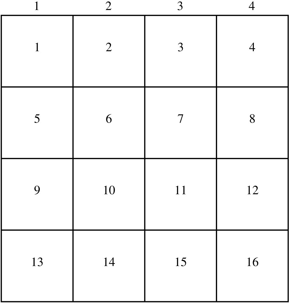 Figure 1
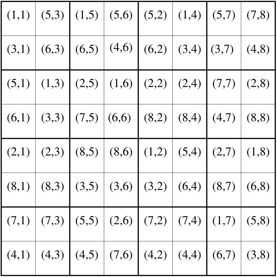 Figure 2