Optimizing stability of mutual synchronization between a pair of limit-cycle oscillators with weak cross coupling
Sho Shirasaka, Nobuhiro Watanabe, Yoji Kawamura, and Hiroya Nakao

TL;DR
This paper develops a method to optimize the linear stability of synchronized states in weakly coupled limit-cycle oscillators by designing the coupling matrix, enhancing synchronization robustness.
Contribution
It introduces a phase reduction-based approach to derive the optimal coupling matrix for maximizing stability under specific constraints.
Findings
Optimal coupling matrices improve synchronization stability.
The method applies to various types of limit-cycle oscillators.
Enhanced stability demonstrated through numerical examples.
Abstract
We consider optimization of linear stability of synchronized states between a pair of weakly coupled limit-cycle oscillators with cross coupling, where different components of state variables of the oscillators are allowed to interact. On the basis of the phase reduction theory, the coupling matrix between different components of the oscillator states that maximizes the linear stability of the synchronized state under given constraints on overall coupling intensity and on stationary phase difference is derived. The improvement in the linear stability is illustrated by using several types of limit-cycle oscillators as examples.
Click any figure to enlarge with its caption.
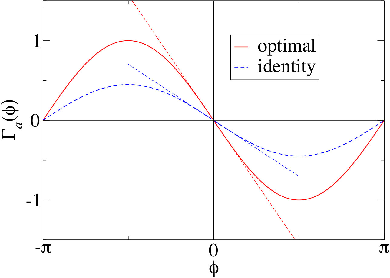 Figure 1
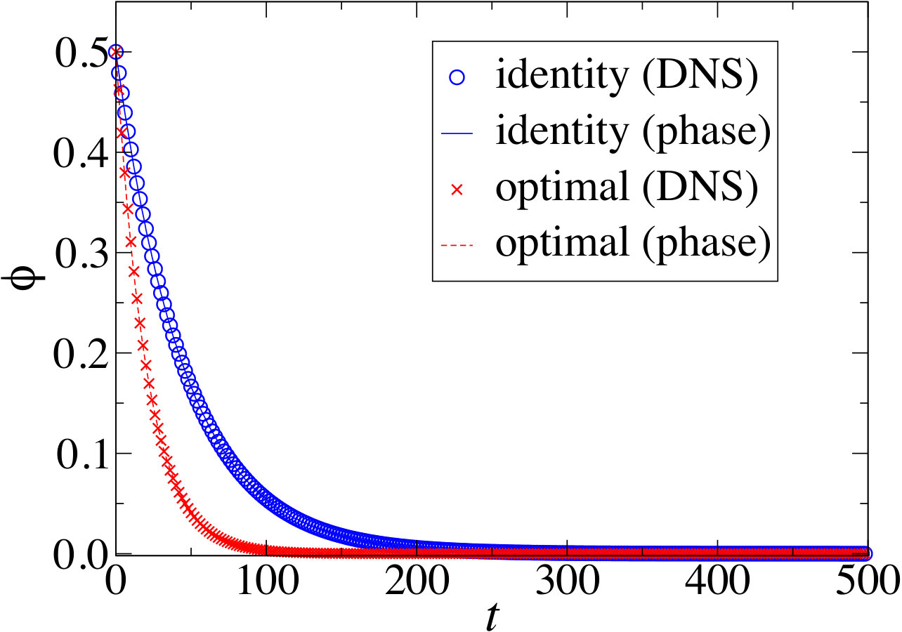 Figure 2
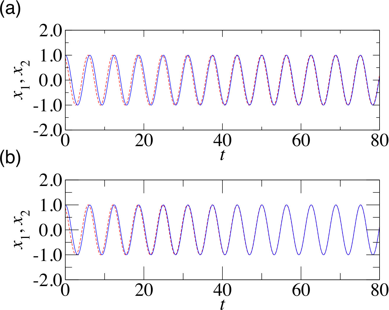 Figure 3
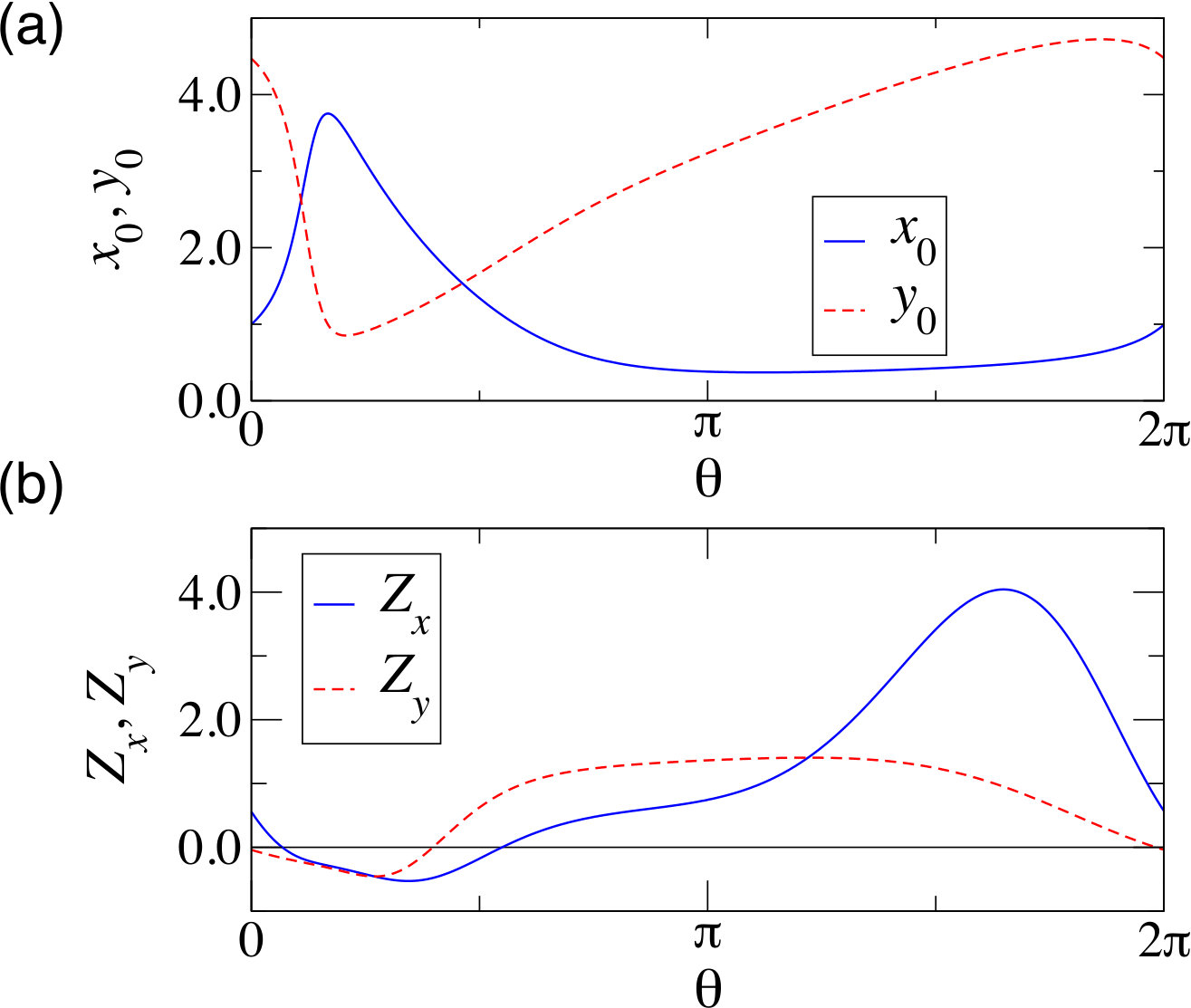 Figure 4
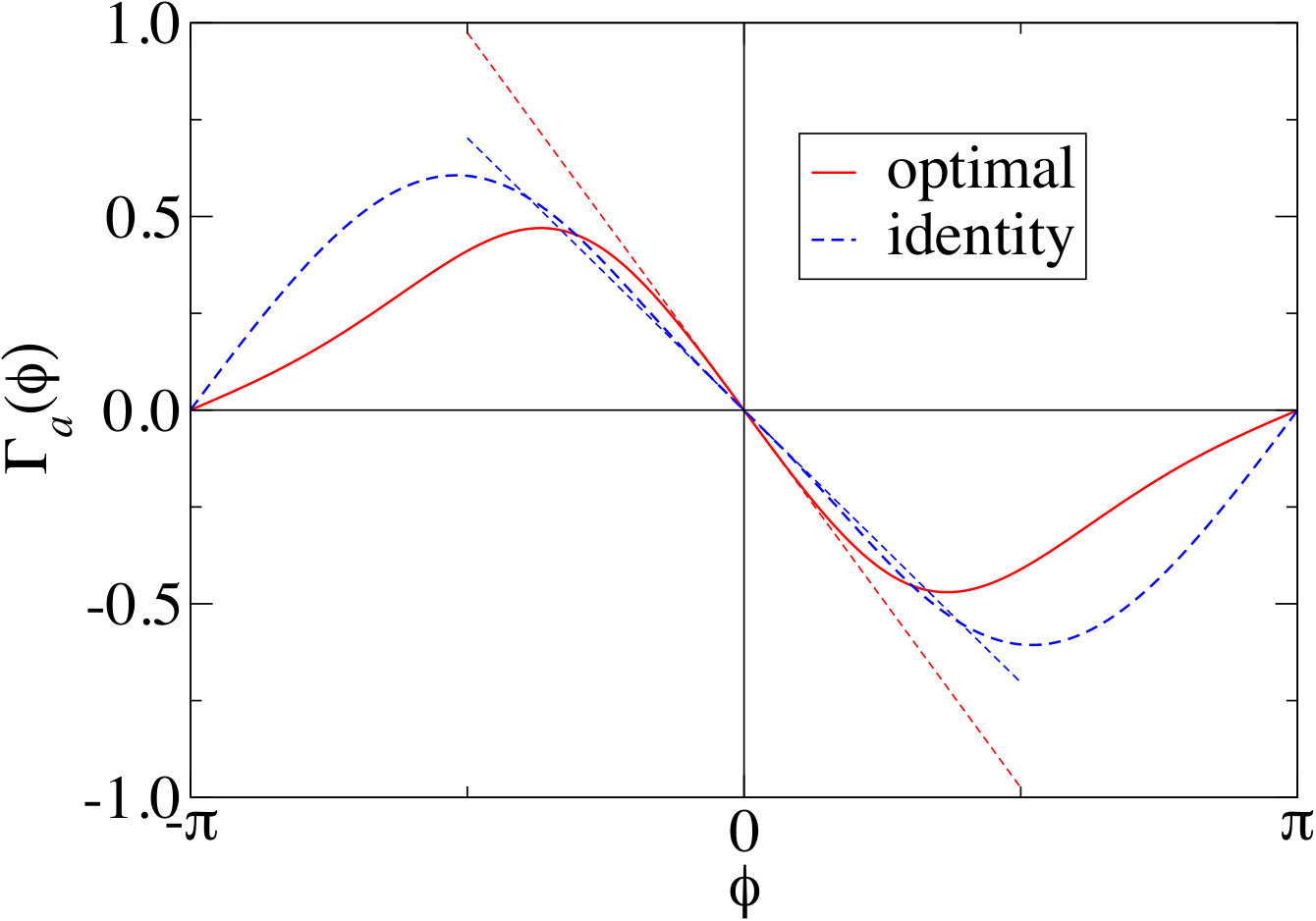 Figure 5
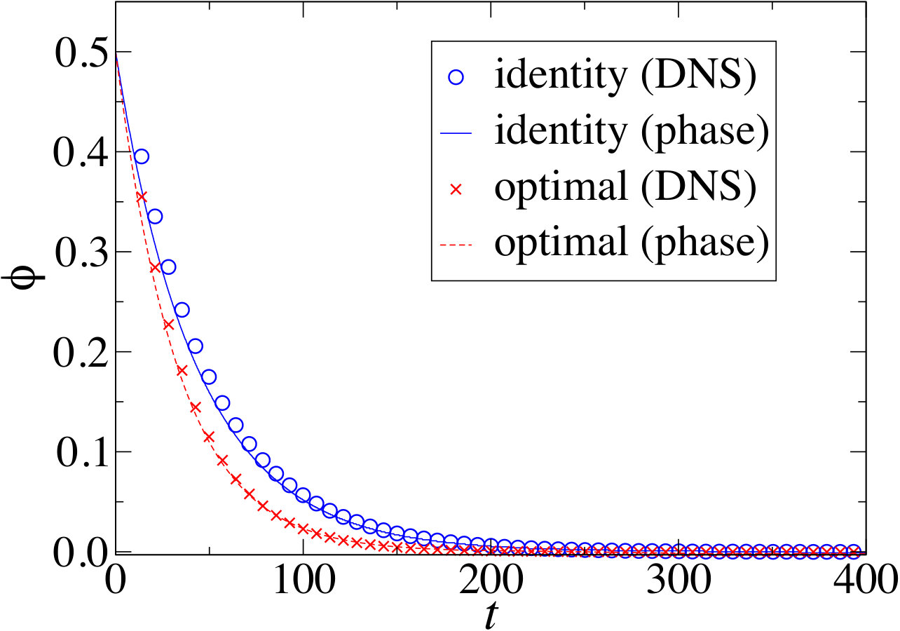 Figure 6
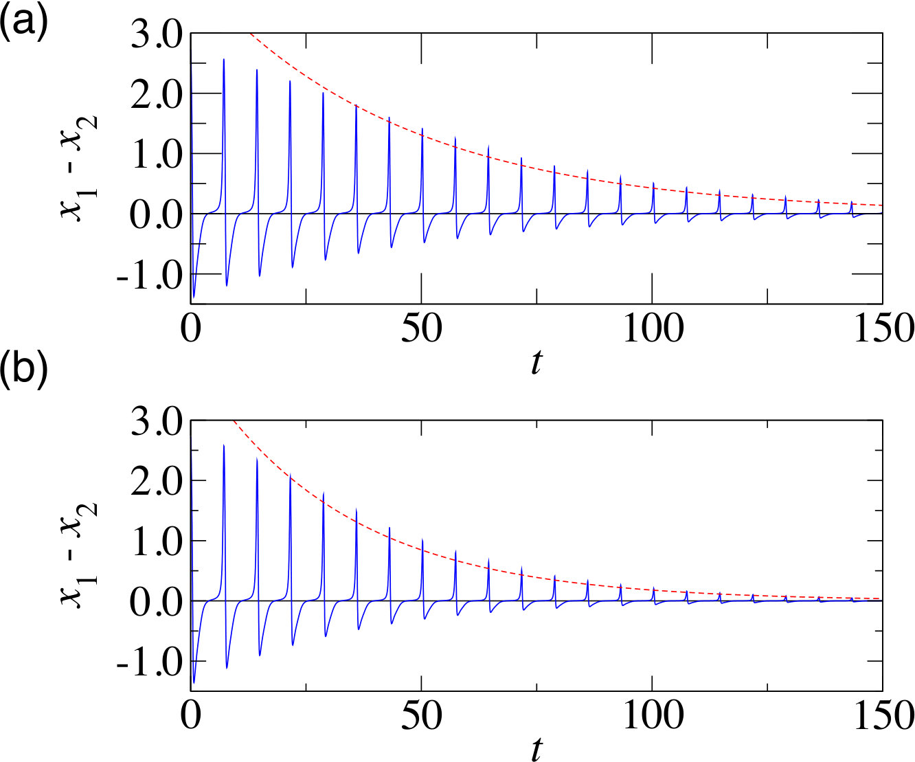 Figure 7
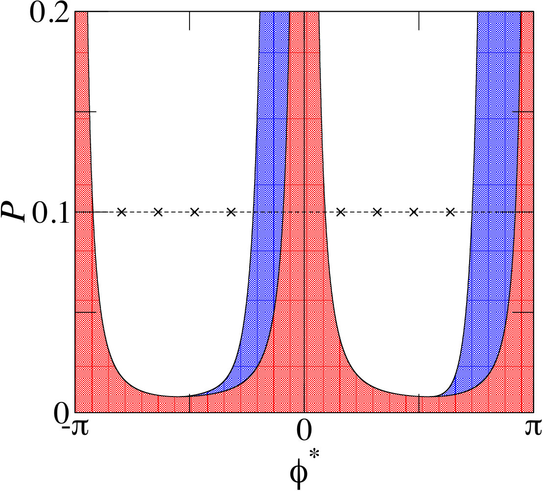 Figure 8
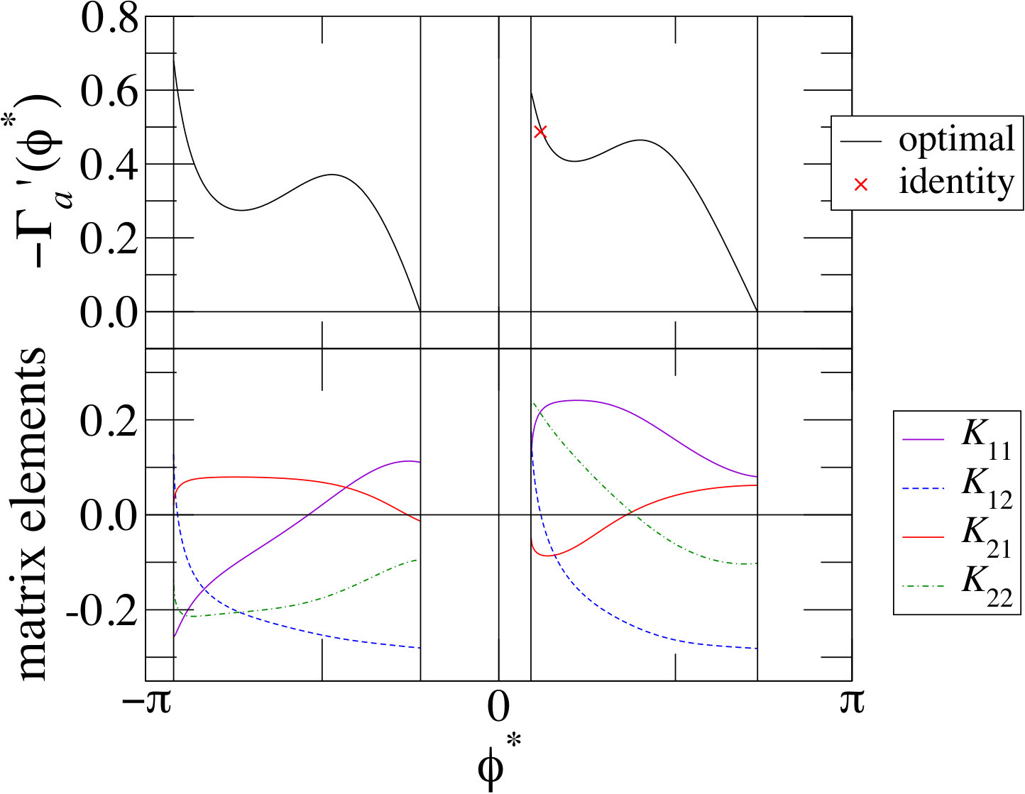 Figure 9
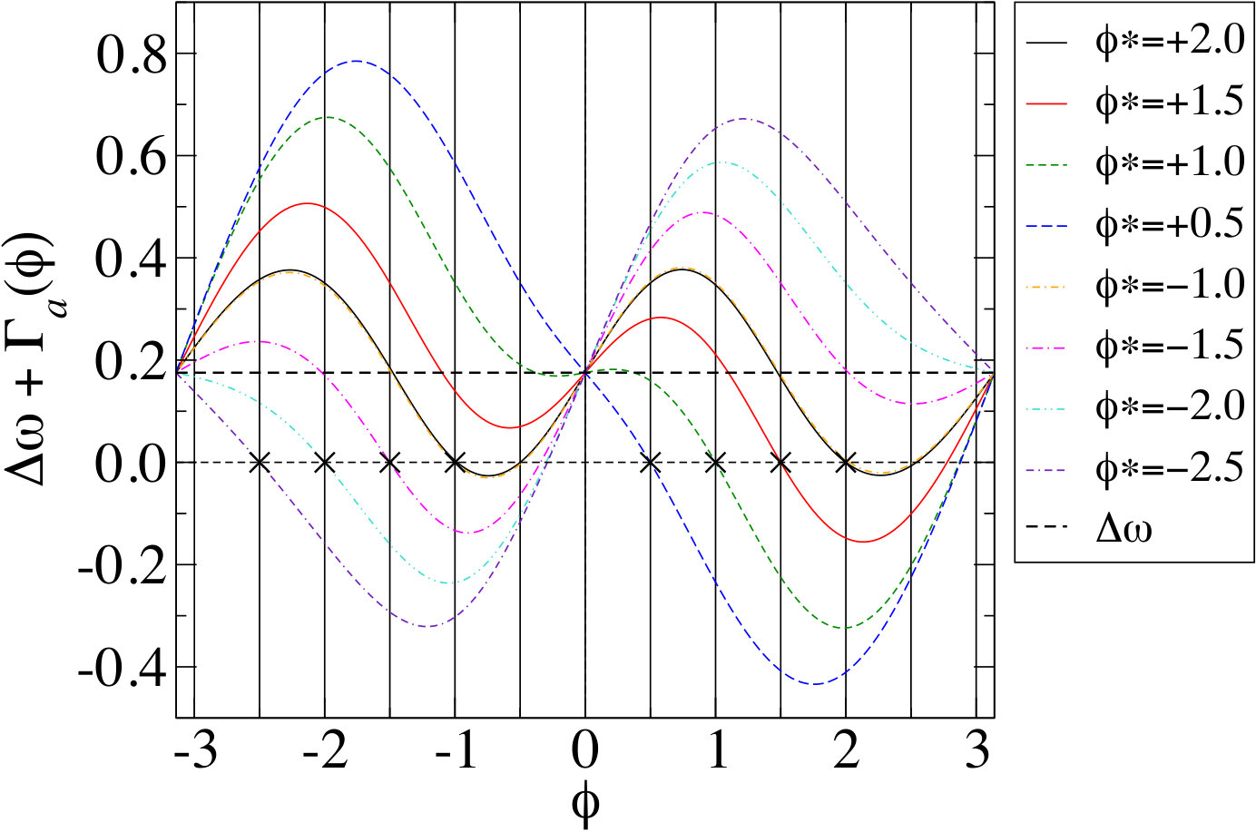 Figure 10
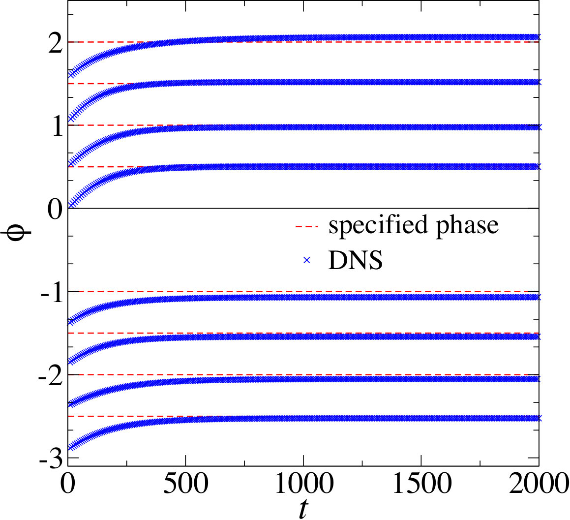 Figure 11
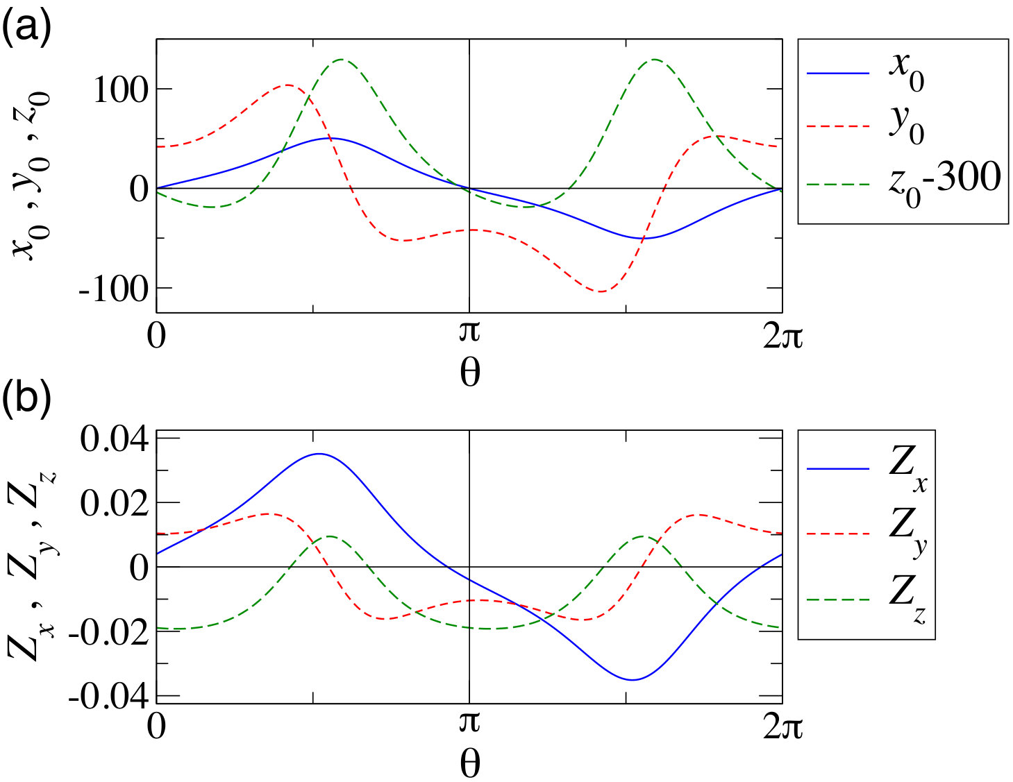 Figure 12
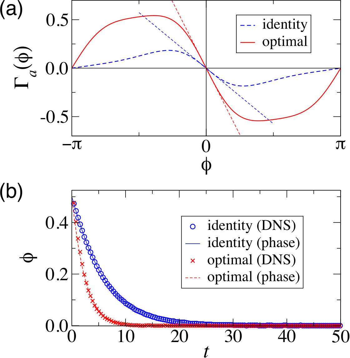 Figure 13
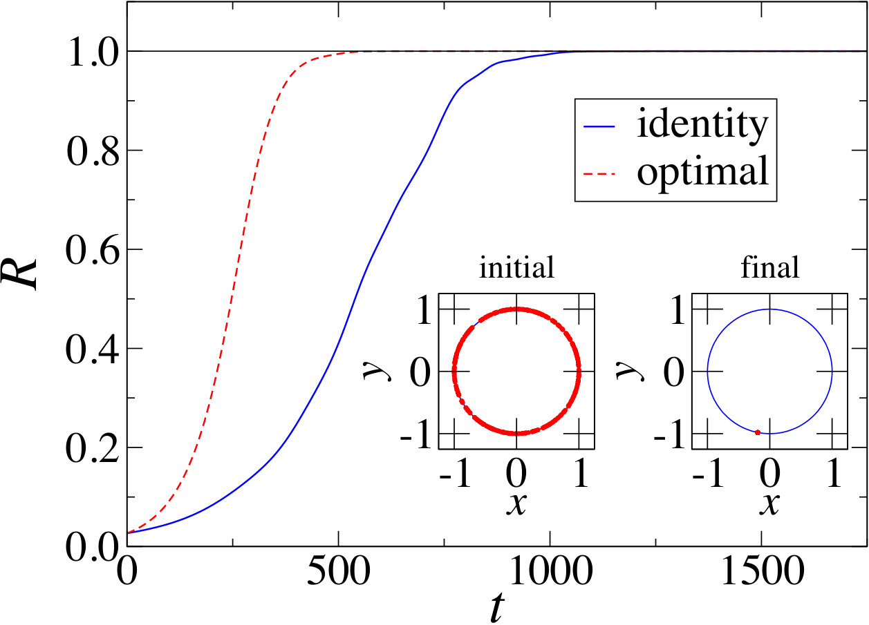 Figure 14
Peer Reviews
No public reviews on file for this paper yet. If you reviewed it on a platform where reviews are public (OpenReview, ICLR, NeurIPS, ICML), you can paste yours below so the community can read it here.
Videos
No videos yet. Explain this paper in a talk, walkthrough, or lecture? Add one.
Optimizing stability of mutual synchronization between a pair of limit-cycle oscillators with weak cross coupling
Sho Shirasaka
Research Center for Advanced Science and Technology, University of Tokyo, Tokyo 153-8904, Japan
Nobuhiro Watanabe
Department of Systems and Control Engineering, Tokyo Institute of Technology, Tokyo 152-8552, Japan
Yoji Kawamura
Department of Mathematical Science and Advanced Technology, Japan Agency for Marine-Earth Science and Technology, Yokohama 236-0001, Japan
Hiroya Nakao
[email protected] (corresponding author)
Department of Systems and Control Engineering, Tokyo Institute of Technology, Tokyo 152-8552, Japan
Department of Mechanical Engineering, University of California, Santa Barbara, California
Abstract
We consider optimization of linear stability of synchronized states between a pair of weakly coupled limit-cycle oscillators with cross coupling, where different components of state variables of the oscillators are allowed to interact. On the basis of the phase reduction theory, the coupling matrix between different components of the oscillator states that maximizes the linear stability of the synchronized state under given constraints on overall coupling intensity and on stationary phase difference is derived. The improvement in the linear stability is illustrated by using several types of limit-cycle oscillators as examples.
pacs:
05.45.Xt
I Introduction
Synchronization of nonlinear oscillators is widely observed and often plays important functional roles in a variety of real-world systems ref:pikovsky01 ; ref:strogatz03 ; strogatz15 ; ref:winfree80 ; Kuramoto ; ref:hoppensteadt97 ; ref:ermentrout10 ; Kiss ; Kiss2 . Exploration of efficient methods for realizing stable synchronization between coupled oscillators or between oscillators and driving signals is both fundamentally and practically important. Improvement in the efficiency of collective synchronization in networks of coupled oscillators has been extensively studied in the literature ref:tanaka08 ; ref:yanagita10 ; ref:yanagita12 ; ref:yanagita14 ; ref:skardal14 ; ref:skardal16 ; ref:nishikawa06a ; ref:nishikawa06b ; ref:nishikawa10 ; Ravoori for both Kuramoto-type phase models and chaotic oscillators, where optimization of coupling networks connecting the oscillators has been the main target.
In the analysis of synchronization dynamics between weakly coupled nonlinear oscillators undergoing limit-cycle oscillations, the phase reduction theory has played a dominant role ref:winfree80 ; Kuramoto ; ref:hoppensteadt97 ; ref:ermentrout10 ; ref:brown04 ; ref:nakao16 ; ref:ashwin16 . It allows us to simplify the dynamics of a pair of limit-cycle oscillators with weak coupling to a simple scalar equation for their phase difference. The phase reduction theory, originally developed for finite-dimensional smooth limit-cycle oscillators, has recently been generalized to non-conventional limit-cycling systems such as collectively oscillating populations of coupled oscillators Kawamura1 , systems with time delay Kotani ; Novicenko1 ; Novicenko2 , reaction-diffusion systems Nakao , oscillatory fluid convection Kawamura2 , and hybrid dynamical systems Shirasaka . Recently, methods for optimizing periodic external driving signals for efficient injection locking and controlling of a single nonlinear oscillator (or a population of uncoupled oscillators) have also been proposed on the basis of the phase reduction theory ref:moehlis06 ; ref:harada10 ; ref:dasanayake11 ; ref:zlotnik12 ; ref:zlotnik13 ; ref:pikovsky15 ; ref:tanaka14a ; ref:tanaka14b ; ref:tanaka15 ; ref:zlotnik2016 ; ref:hasegawa14a ; ref:hasegawa14b . In this study, we consider a pair of coupled limit-cycle oscillators and try to optimize the linear stability of the synchronized state using the phase reduction theory.
In the analysis of mutual synchronization of coupled oscillators, linear diffusive coupling between the oscillators is a common setup. However, in most cases, only the same vector component of the state variables can interact between the oscillators and different vector components of the oscillator states are usually not allowed to interact. In this study, we analyze a pair of oscillators with weak cross coupling, where different vector components of the oscillator states are allowed to interact, that is, differences in each vector component of the oscillator states can be feed-backed to every other component with a linear gain specified by a coupling matrix, and optimize the coupling matrix so that the linear stability of the mutually synchronized state is maximized.
We use the phase reduction theory to simplify the dynamics of a pair of weakly coupled limit-cycle oscillators to a scalar equation for the phase difference, and use the method of Lagrange multipliers to derive the optimal coupling matrix for the cases with and without frequency mismatch between the oscillators. Using three examples of simple limit-cycle oscillators, we illustrate that the linear stability of the synchronized state is actually improved and also that the stationary phase difference can be controlled by appropriately choosing the coupling matrix.
This paper is organized as follows: in Sec. II, we introduce the coupled-oscillator model and derive the equation for the phase difference by using the phase reduction theory. In Sec. III, we formulate the optimization problem for improving linear stability of the phase-locked states. In Sec. IV, the theoretical results are illustrated by several examples of limit-cycle oscillators. Sec. V gives summary and discussion.
II Model
In this section, we introduce a pair of nearly identical limit-cycle oscillators with weak cross coupling, reduce the dynamical equations to coupled phase equations by using the phase reduction theory ref:winfree80 ; Kuramoto ; ref:hoppensteadt97 ; ref:brown04 ; ref:ermentrout10 ; ref:nakao16 ; ref:ashwin16 , and derive the equation for the phase difference.
II.1 A pair of cross-coupled oscillators
We consider a pair of weakly and symmetrically coupled, nearly identical limit-cycle oscillators described by
[TABLE]
where and are the -dimensional state vectors of the oscillators and , respectively, and are -dimensional vector-valued functions representing the dynamics of the oscillators, is a matrix of coupling intensities between the components of the state variables, and is a small positive parameter indicating that the interaction is sufficiently small.
Here, although the oscillators are “diffusively” coupled, we assume that the matrix is generally not diagonal and can possess non-diagonal elements. That is, differences in each vector component of the oscillator states are returned to other components as feedback signals with appropriate gains. Therefore, different components of the state variables of the oscillators can mutually interact. This gives the possibility to improve the stability of the synchronized state by adjusting the non-diagonal elements of the coupling matrix, exceeding the stability that is achievable only with the diagonal coupling. We assume linear diffusive coupling in the following, but the argument can be straightforwardly generalized to nonlinear coupling; see Sec. V.
We assume that the properties of the oscillators are nearly identical and their difference is . That is, the functions can be split into a common part and deviations as
[TABLE]
where , , and are assumed to be . We also assume that the common part of the oscillator dynamics, , possesses a stable limit-cycle solution of period and frequency , and that the dynamics of the oscillator is only slightly deformed and persists even if small perturbations from the deviations and mutual coupling are introduced. These assumptions are necessary for the phase reduction that we rely on in the present study.
II.2 Phase reduction
Under the above assumptions, we can simplify the dynamics of the coupled oscillators to coupled phase equations by applying the phase reduction theory ref:winfree80 ; Kuramoto ; ref:hoppensteadt97 ; ref:brown04 ; ref:ermentrout10 ; ref:nakao16 ; ref:ashwin16 . That is, we introduce a phase () of the oscillator state near the limit-cycle solution that increases with a constant frequency in the absence of perturbations, and represent the oscillator state on the limit cycle as a function of the phase as .
In the present case, we introduce phase variables of the two oscillators, represent the oscillator states near the limit-cycle orbit as as functions of at , and approximately describe their dynamics by using only . By following the standard phase reduction and averaging procedures, we can derive a pair of coupled phase equations, which is correct up to , as
[TABLE]
The frequencies of the oscillators are given by
[TABLE]
and the phase coupling function is given by
[TABLE]
Here, we introduced an abbreviation for the average over phase from [math] to ,
[TABLE]
where is a -periodic function of . In the following, without loss of generality, we assume that , and denote the frequency difference between the oscillators as , where is .
The function in Eqs. (7) and (9) is a phase sensitivity function of the limit cycle of the common part, . It is given by a -periodic solution to the adjoint equation , where is a Jacobi matrix of the vector field at and T denotes the matrix transpose, and is normalized as . By using the adjoint method by Ermentrout ref:ermentrout10 ; ref:brown04 ; ref:nakao16 , i.e., by backwardly evolving the adjoint equation with occasional renormalization, can be calculated numerically.
For convenience, we rewrite the phase coupling function as
[TABLE]
where
[TABLE]
is a correlation matrix between the vector components of the phase sensitivity function and the state difference between the oscillators. Here, the symbol represents a tensor product and denotes the trace of a matrix. See Appendix A for the definition and related matrix formulas. Because and are -periodic functions, and are also -periodic.
II.3 Stability of the synchronized state
From Eq. (5), the phase difference (restricted to hereafter) between the two oscillators obeys
[TABLE]
Here, is the antisymmetric part of the phase coupling function ; it is also -periodic and satisfies . Therefore, if satisfies , Eq. (14) has at least one stable fixed point at the phase differences satisfying . We denote one of such fixed points as .
From Eq. (14), the linear stability of is given by , where is the slope of at . Thus, if a fixed point satisfies
[TABLE]
and
[TABLE]
the phase difference can take a stationary phase difference, and the two oscillators can mutually synchronize, or phase-locked to each other, with a stable phase difference (within the phase-reduction approximation).
By defining a new matrix
[TABLE]
the antisymmetric part of the phase coupling function and its slope can be expressed as
[TABLE]
where represents derivative of with respect to . Using -periodicity of and , the matrices and can be expressed as
[TABLE]
and
[TABLE]
where the derivative of with respect to is given by
[TABLE]
See Appendix B for the calculations. We use these expressions in the next section.
III Optimizing the coupling matrix
In this section, we derive the optimal coupling matrix for stable synchronization (phase locking) of the two oscillators.
III.1 Optimality condition and constraint on the coupling matrix
Our aim is to maximize the linear stability of the synchronized (phase-locked) state, characterized by , by adjusting the coupling matrix . Other types of optimality conditions for synchronization have also been considered in the literature for nonlinear oscillators driven by periodic signals, such as maximization of frequency difference between the oscillator and signal for fixed coupling intensity ref:harada10 ; ref:tanaka14a and minimization of the phase diffusion constant under the effect of noise ref:pikovsky15 , in addition to the maximization of linear stability ref:dasanayake11 ; ref:zlotnik12 ; ref:zlotnik13 that we generalize to coupled oscillators in the present study footnote .
We first consider the simple case where the two oscillators are identical and share the same frequency, and optimize the stability of the in-phase synchronized state with zero phase difference, . We then consider the general case with a frequency mismatch and optimize the stability of the synchronized state with a given stationary phase difference , which is not necessarily [math]. In both cases, as a constraint on the overall connection intensity between the oscillators, we fix the Frobenius norm (see Appendix A) of the coupling matrix as , where is a given constant. In the latter case, the stationary phase difference is also constrained.
III.2 Optimization for identical oscillators without frequency mismatch
We first consider the simple case where the oscillators are identical, , and their frequencies are equal to each other, and . In this case, the in-phase and anti-phase synchronized states and are always stationary solutions to Eq. (14) because .
We thus try to find the coupling matrix that gives the maximum of linear stability of ,
[TABLE]
subject to the constraint on the Frobenius norm of ,
[TABLE]
Because , we divide this quantity by and simply try to maximize
[TABLE]
which we also call “linear stability” for simplicity in the following. We introduce an action,
[TABLE]
where is a Lagrange multiplier. The first term of represents the stability of the fixed point and the second term represents the constraint.
By differentiating by and , we obtain
[TABLE]
and the constraint . Therefore, the optimal should satisfy
[TABLE]
Plugging this into Eq. (24) yields
[TABLE]
It turns out that the negative sign should be chosen (see Eq. (33)), so that the optimal coupling matrix is given by
[TABLE]
The antisymmetric part of the phase coupling function with this is given, from Eq. (18), by
[TABLE]
and the optimal linear stability of the in-phase fixed point is given by
[TABLE]
III.3 Optimization for nonidentical oscillators with frequency mismatch
We next consider the general case with nonidentical oscillators with a frequency mismatch . We constrain the Frobenius norm of as as before, and also require that the given satisfies Eq. (36), i.e., , so that is actually the stationary phase difference of the oscillators.
We thus seek for the optimal coupling matrix that maximizes
[TABLE]
now for a given stationary phase difference , subject to
[TABLE]
and
[TABLE]
Here, we exclude the cases with and , because these states can never be realized when as we argue later (the case with and was already considered in the previous subsection, and and can be analyzed similarly).
Using Lagrange multipliers and , we introduce an action (in the rest of this subsection, shorthand notations and are used),
[TABLE]
Differentiating by , , and , we obtain
[TABLE]
and the two constraints, Eqs. (36) and (24). Thus, the optimal should satisfy
[TABLE]
and plugging this into Eq. (36) yields
[TABLE]
Solving this equation for , we obtain
[TABLE]
and therefore
[TABLE]
where has yet to be determined from the constraint on the Frobenius norm.
Plugging this into and using , we obtain
[TABLE]
which gives
[TABLE]
It turns out that the minus sign should be chosen to maximize the linear stability (see below).
Note here that holds by the Schwartz inequality (see Appendix A), so the condition
[TABLE]
is necessary for and hence to exist. Note also that
[TABLE]
should hold strictly for the existence of in Eq. (45), that is, should not be equal to , because then and does not exist. Therefore, the optimization problem cannot be solved in the case that and are parallel to each other.
The antisymmetric part of the phase coupling function for is given by
[TABLE]
and the maximal possible linear stability is given by
[TABLE]
Because and , the first term is positive only when . Therefore, the minus sign should be chosen for in Eq. (47) to realize the maximal stability, and the optimal coupling matrix is given by Eq. (45) with the negative .
Note that even if we choose the minus sign for , the above quantity can still be negative if the second term on the right-hand side is negative, i.e., . If so, the fixed point with phase difference is unstable and cannot be realized. Thus, in this case, as can be shown by comparing the two terms on the right-hand side of Eq. (55), should additionally satisfy
[TABLE]
for to be linearly stable.
Depending on the conditions, the present optimization problem may or may not possess an appropriate solution. For example, when , it is impossible to realize completely in-phase () or anti-phase () synchronization, because satisfies , so can never be satisfied at or . Also, when , it is generally difficult (very large is required) to realize the synchronized state with a stationary phase difference very close to [math] or . This will be illustrated in the next section. The equation may also have multiple solutions, so not only the fixed point with the given phase difference but also spurious fixed points with other phase differences may arise.
IV Examples
In this section, we illustrate the improvement in the linear stability of coupled oscillators by optimizing with a few types of limit-cycle oscillators as examples.
IV.1 Stuart-Landau oscillator
As the first example, we consider the Stuart-Landau (SL) oscillator, a normal form of the supercritical Hopf bifurcation Kuramoto . All necessary quantities can be analytically calculated for this model. The SL oscillator has a two-dimensional state variable, , whose dynamics is specified by a vector field
[TABLE]
where and are parameters. It possesses a single stable limit-cycle orbit of frequency given by
[TABLE]
with (mod ). The phase sensitivity function of this limit cycle can be explicitly calculated as Kuramoto ; ref:nakao16
[TABLE]
We consider a pair of symmetrically coupled SL oscillators with identical properties obeying Eq. (2), which is explicitly described by
[TABLE]
where and are the state variables of the oscillators. The frequency of the oscillators in the absence of mutual coupling is given by .
From Eqs. (66) and (71), the matrix and its derivative can be calculated as
[TABLE]
and
[TABLE]
so they are parallel to each other.
Because the oscillators are identical, and , the in-phase synchronized state always exists. From Eq. (31), the stability of this state can be maximized by choosing as
[TABLE]
and the maximum possible linear stability is given, from Eq. (33), by
[TABLE]
For comparison, suppose that the coupling matrix is a multiple of the identity matrix with the same Frobenius norm as , i.e.,
[TABLE]
which we call the “identity coupling” hereafter. The linear stability of with this is given by
[TABLE]
so the linear stability improves by a factor of by using the optimal coupling matrix from the case with .
Figure 1 shows the antisymmetric part of the phase coupling function calculated for coupling matrices and , with parameters and and overall coupling intensity . It can be seen that the linear stability of the in-phase fixed point is higher in the case with than in the case with . Figure 2 compares the time courses of the phase difference from the initial condition for and obtained by direct numerical simulations of the coupled SL oscillators and by numerical integration of the reduced phase equation. Figure 3 shows the synchronization dynamics obtained numerically, where the components of the two oscillators are shown for and . It can be seen that the oscillators synchronize faster in the case with , reflecting higher linear stability of , than in the case with .
It is interesting to note that when , that is, when the instantaneous frequency of the SL oscillator does not depend on its amplitude, is already optimal and no improvement can be made by introducing cross coupling between different variables of the oscillators.
For nonidentical SL oscillators with a small parameter mismatch , the antisymmetric part of the phase coupling function and its derivative take the form and from Eqs. (18), (92) and (95), where is a constant determined by and ( should also satisfy ). Once the stationary phase difference is specified, the constant is determined as and the linear stability of is given by a fixed value . Therefore, we cannot consider further optimization of the stability for the coupled SL oscillators. Indeed, we cannot consider the second case in Sec. III, because and , given by Eqs. (92) and (95), are strictly parallel to each other, so the Lagrange multiplier vanishes and does not exist. This is a peculiar property of the SL oscillator with purely sinusoidal limit cycles and phase sensitivity functions.
IV.2 Brusselator
As the second example, we use the Brusselator model of chemical oscillations Kuramoto . It has a two-dimensional state variable, , which obeys
[TABLE]
where and are parameters. When and , the period of the oscillation is . Figure 4 shows the limit-cycle solution and the phase sensitivity function for obtained numerically. Other quantities such as and can also be numerically calculated from these and .
We consider a pair of Brusselators with parameters , where is a small number representing parameter mismatch, and couple them in the same way as in the previous SL case, Eq. (89). We seek for the optimal that gives the maximum stability of the synchronized state, and compare the results for with those for the identity coupling, i.e., given by Eq. (102). The overall intensity is fixed at in the following.
We first consider the case without parameter mismatch, . The frequencies of the oscillator are identical in this case, . The optimal and identity coupling matrices with are calculated as
[TABLE]
We can see that, in the optimal case, the feedback from the difference in component to the dynamics of and components is stronger than that in the opposite direction. This reflects the waveforms of the oscillation and phase sensitivity function, in particular, that the variation in is generally larger than that in , as shown in Fig. 4.
Figure 5 shows the antisymmetric part of the phase coupling function for and . The linear stability of the in-phase synchronize state is approximately for and for . Figure 6 shows the evolution of phase differences for and obtained by direct numerical simulations of the coupled Brusselators and by numerical integration of the reduced phase model. The parameter is fixed at in the numerical simulations. Figure 7 shows the synchronization processes of the Brusselators, where time courses of the differences in components between the oscillators, i.e., , are plotted for and . For comparison, an exponentially decaying curve with the decay rate is also shown in each figure. It can been seen that in-phase synchronization is established faster when is used, and the exponential decay rate of the state difference matches with the linear stability of .
We next consider the case with parameter mismatch, . The frequencies of the oscillators are () and (). We assume in the following calculations, so the frequency mismatch parameter is . Using the results obtained in the previous section, we calculate the optimal coupling matrix for a given phase difference in .
Figure 8 shows the necessary conditions for given by Eq. (48) and Eq. (56) as functions of the phase difference for , where the latter applies only when . Both conditions are satisfied in the non-shaded regions. We see that should not be too small and that the regions near and are difficult to realize, as argued in the previous section.
Figure 9 shows the elements of the optimal coupling matrix and the corresponding stability of the fixed point as functions of the phase difference . For comparison, the results for , which gives a stable phase difference and negative slope , are also indicated in the figure. In this particular example, yields reasonably high stability close to the negative slope with the optimal coupling matrix at footnote2 . In the blank regions where the data are not shown, any of the necessary conditions is not satisfied. The stability varies with and, in this case, nearly anti-phase synchronized state yields the highest stability. Elements of the coupling can be positive or negative depending on .
Figure 10 shows the antisymmetric parts of the obtained phase coupling functions for given phase differences, , and . The given phase differences are actually realized with the optimal as stable fixed points. From this figure, we can clearly see why stationary phase differences close to [math] or are difficult to realize, in consistent with the conditions shown in Fig. 8. Figure 11 plots the results of direct numerical simulations for coupled Brusselators using the optimal coupling matrices , where the convergence of the phase differences to given values is shown.
IV.3 Lorenz model
Finally, as a simple three-dimensional example, we consider the Lorenz model in the limit-cycling regime strogatz15 , whose state variable evolves with the vector field
[TABLE]
with , , and . The frequency of the limit-cycle oscillation is . Figure 12 shows the evolution of for one period of oscillation and the corresponding phase sensitivity function obtained by the adjoint method ref:ermentrout10 .
We consider two Lorenz models without frequency mismatch and couple them via the coupling matrix as in Eq. (2). We compare the results for the optimal coupling matrix with those for . From the results in the previous section, for , and are estimated as
[TABLE]
and
[TABLE]
The linear stability is approximately for the optimal coupling and for the identity coupling, respectively. Figure 13 shows the antisymmetric parts of the phase coupling functions for and , and compares the time courses of the phase differences obtained numerically for . We can clearly see that the stability of the in-phase state is higher and correspondingly the phase difference decays to zero faster in the optimal case.
It is notable that has several zero components, indicating no feedback from component to or component nor from or component to component arise even after optimization. This is because component exhibits qualitatively different dynamics from those of and components in the Lorenz model. As can be seen from Fig. 12, the fundamental frequency of component is exactly twice that of and components. Reflecting the symmetry of the Lorenz model (invariance under , , ), the waveforms of and exhibit the same pulse-like oscillations exactly twice while other quantities, , , , and , undergo one period of smooth oscillation that is symmetric to . Therefore, when averaged over one period, feedback from to or (characterized by or multiplied by the difference in components) vanishes and does not help improve the stability of the synchronized state for the coupled Lorenz oscillators. Similarly, feedback from or to (characterized by multiplied by the difference in or ) does not contribute to the stability.
V Summary and discussion
We have considered a pair of limit-cycle oscillators with weak cross coupling, where different components of the oscillator states are allowed to interact, and optimized the coupling matrix so that the stability of the synchronized state is improved. For oscillators without frequency mismatch, the optimal coupling matrix yields higher linear stability of the in-phase synchronized state. For oscillators with frequency mismatch, a range of phase-locked state with given stationary difference can be realized by choosing the coupling matrix appropriately. Necessary conditions for realizability of a given phase difference are also derived.
In this paper, we have derived the optimal coupling matrix that yields the highest linear stability of the synchronized state for linear diffusive coupling given by Eq. (2). This result can be straightforwardly extended to coupled oscillators with general coupling functions, described by
[TABLE]
where represents general nonlinear coupling between the oscillators and . In this case, the phase coupling function in the reduced phase equations (5) is given by
[TABLE]
instead of Eq. (9). Thus, by defining the function as
[TABLE]
in place of Eq. (13) and calculating and from this , the optimization can be performed in a similar way to the linear diffusive case. For example, the optimal coupling matrix for the case without frequency mismatch is given by Eq. (31) with the above .
Also, though we have considered only the simple case where all components of the oscillator states can interact with all other components in this paper, it is straightforward to restrict the pairs of components that can actually interact by constraining certain components of to zero, in order to incorporate realistic physical situations. It would also be interesting to generalize the theory to incorporate different constraints on , for example, to reduce the number of non-zero components by assuming sparsity constraint on .
Although we have considered only the most fundamental two-oscillator problem in this paper, synchronization of a network of many oscillators have attracted much attention Kiss ; Kiss2 ; ref:tanaka08 ; ref:yanagita10 ; ref:yanagita12 ; ref:yanagita14 ; ref:skardal14 ; ref:skardal16 ; ref:nishikawa06a ; ref:nishikawa06b ; ref:nishikawa10 ; Ravoori ; Dorfler ; LiWong ; Stankovski , and generalization of the present framework to many-oscillator networks would be an interesting future problem. For the simplest globally coupled population of identical oscillators described by
[TABLE]
it is expected that the optimal coupling matrix for the two-oscillator case would also provide faster convergence to global synchrony than the identity coupling matrix. To illustrate this, we simulated SL oscillators with the same parameter values as in Sec. IV, starting from uniformly random initial conditions on the limit cycle. Figure 14 shows synchronization processes for and for in Eqs. (98) and (102), where evolution of the modulus of the Kuramoto order parameter, estimated by , is plotted. We can observe that the oscillators exhibit much faster convergence to complete synchrony () with than with , as expected. Of course, for more complex oscillator networks with frequency heterogeneity and coupling randomness, the result of optimization for the two-oscillator case would not apply due to many-body effects and further investigation should be necessary.
Finally, synchronization between spatiotemporal rhythms in chemical systems has been studied recently ref:mikhailov06 ; ref:mikhailov13 ; ref:mikhailov14 ; hildebrand ; Fukushima ; Epstein , and generalization of the phase reduction theory to reaction-diffusion equations exhibiting stable spatiotemporal oscillations has also been performed Nakao . The present framework can also be extended to such situations and can be used to derive the optimal coupling schemes between two coupled spatiotemporal oscillations. A study in this direction is reported in our forthcoming article kawamura , where improvement in the stability of synchronized states between reaction-diffusion systems by introducing linear spatial filters into mutual coupling is considered.
Acknowledgements.
S.S. acknowledges financial support from JSPS (Japan) KAKENHI Grant Number JP15J12045. Y.K. acknowledges financial support from JSPS (Japan) KAKENHI Grant Number JP16K17769. H.N. acknowledges financial support from JSPS (Japan) KAKENHI Grant Numbers JP16H01538, JP16K13847, and JP17H03279.
Appendix
V.1 Matrix formulas
The tensor product of -dimensional vectors and gives a matrix whose -component is for . The inner product of matrices and is defined as
[TABLE]
where and represent -components of the matrices and , respectively. The Frobenius norm of a matrix is defined as
[TABLE]
and the inner product of the matrices and is defined as
[TABLE]
Derivative of the inner product of matrices is given by
[TABLE]
and derivative of the Frobenius norm is given by
[TABLE]
For arbitrary matrices and , the Schwartz inequality
[TABLE]
holds, which can be shown by plugging into an inequality that holds for arbitrary .
V.2 Calculation of and
Using and , is explicitly given as
[TABLE]
From this , the function can be calculated as
[TABLE]
where -periodicity of the functions and was used. Similarly, the derivatives of and can be calculated as
[TABLE]
and
[TABLE]
where -periodicity was used again. Therefore, the derivative of can be calculated as
[TABLE]
The reference list from the paper itself. Each links out to its DOI / PubMed record.
- 1(1) A. Pikovsky, M. Rosenblum, and J. Kurths, Synchronization: A Universal Concept in Nonlinear Sciences (Cambridge University Press, Cambridge, 2001).
- 2(2) S. H. Strogatz, Sync: How Order Emerges from Chaos in the Universe, Nature, and Daily Life (Hyperion Books, New York, 2003).
- 3(3) S. H. Strogatz, Nonlinear Dynamics and Chaos, 2nd ed. (Westview Press, Boulder, 2015).
- 4(4) A. T. Winfree, The Geometry of Biological Time (Springer, New York, 1980; Springer, Second Edition, New York, 2001).
- 5(5) Y. Kuramoto, Chemical Oscillations, Waves, and Turbulence (Springer, New York, 1984; Dover, New York, 2003).
- 6(6) F. C. Hoppensteadt and E. M. Izhikevich, Weakly Connected Neural Networks (Springer, New York, 1997).
- 7(7) G. B. Ermentrout and D. H. Terman, Mathematical Foundations of Neuroscience (Springer, New York, 2010).
- 8(8) I. Z. Kiss, Y. Zhai, and J. L. Hudson, Emerging coherence in a population of chemical oscillators, Science 296 , 1676 (2002).