Batch Data Processing and Gaussian Two-Armed Bandit
Alexander V. Kolnogorov

TL;DR
This paper analyzes the Gaussian two-armed bandit problem in batch data processing, showing that large packet sizes can be used without significant loss in control performance, especially when processing methods have similar efficiencies.
Contribution
It introduces a model for batch processing in the two-armed bandit framework and quantifies the impact of packet size and method efficiency differences on control risk.
Findings
Large packet processing does not significantly increase minimax risk when methods are similarly efficient.
Initial small-sized packets can mitigate losses when method efficiencies differ.
Control performance remains robust with sufficiently large packet numbers.
Abstract
We consider the two-armed bandit problem as applied to data processing if there are two alternative processing methods available with different a priori unknown efficiencies. One should determine the most effective method and provide its predominant application. Gaussian two-armed bandit describes the batch, and possibly parallel, processing when the same methods are applied to sufficiently large packets of data and accumulated incomes are used for the control. If the number of packets is large enough then such control does not deteriorate the control performance, i.e. does not increase the minimax risk. For example, in case of 50 packets the minimax risk is about 2% larger than that one corresponding to one-by-one optimal processing. However, this is completely true only for methods with close efficiencies because otherwise there may be significant expected losses at the initial stage…
Click any figure to enlarge with its caption.
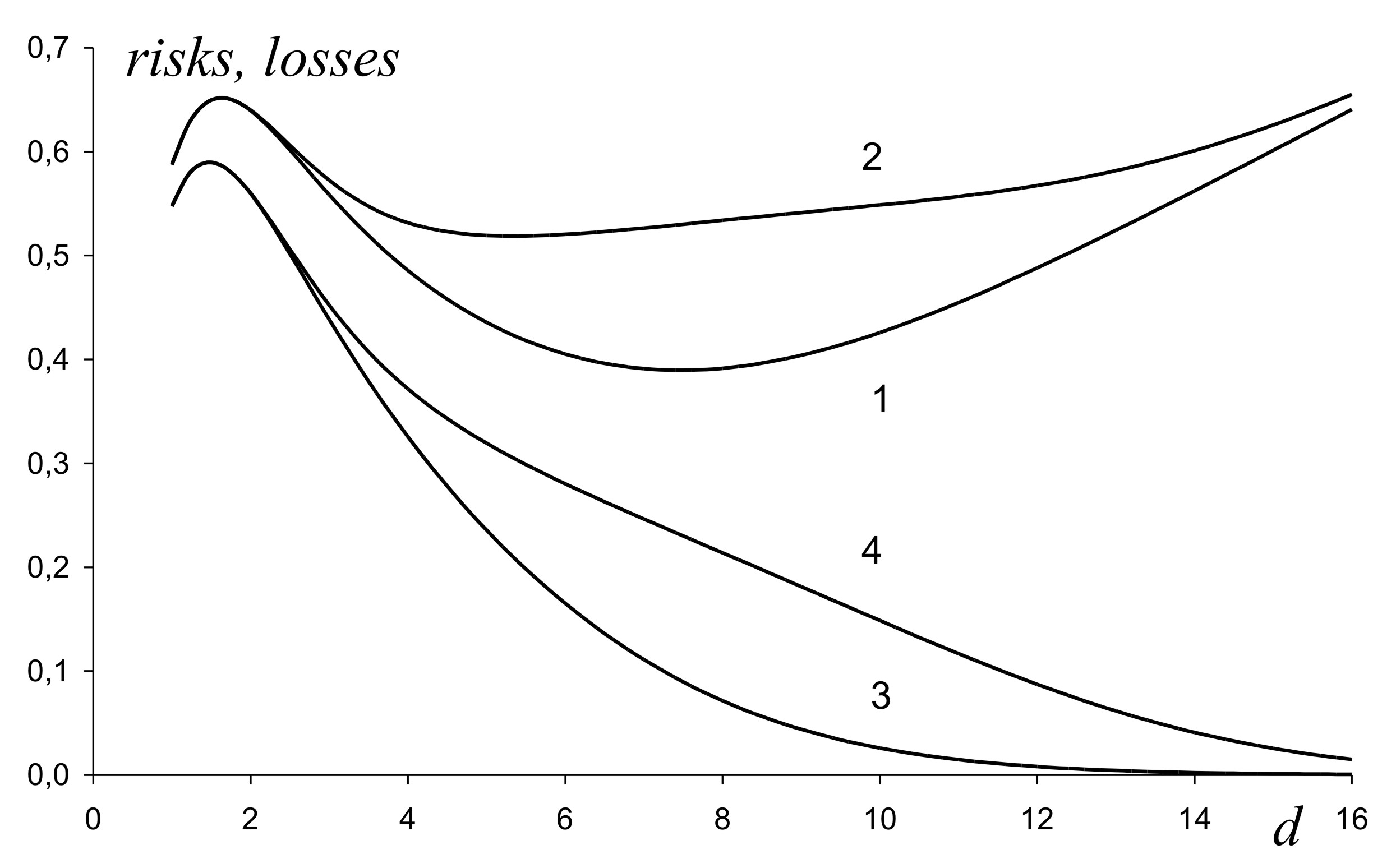 Figure 1
Peer Reviews
No public reviews on file for this paper yet. If you reviewed it on a platform where reviews are public (OpenReview, ICLR, NeurIPS, ICML), you can paste yours below so the community can read it here.
Videos
No videos yet. Explain this paper in a talk, walkthrough, or lecture? Add one.
Taxonomy
TopicsAdvanced Bandit Algorithms Research · Data Stream Mining Techniques
Batch Data Processing
and Gaussian Two-Armed Bandit
Alexander V. Kolnogorov
Yaroslav-the-Wise Novgorod State University, Velikiy Novgorod, 173003 Russia, (e-mail: [email protected]).
Abstract
We consider the two-armed bandit problem as applied to data processing if there are two alternative processing methods available with different a priori unknown efficiencies. One should determine the most effective method and provide its predominant application. Gaussian two-armed bandit describes the batch, and possibly parallel, processing when the same methods are applied to sufficiently large packets of data and accumulated incomes are used for the control. If the number of packets is large enough then such control does not deteriorate the control performance, i.e. does not increase the minimax risk. For example, in case of 50 packets the minimax risk is about 2% larger than that one corresponding to one-by-one optimal processing. However, this is completely true only for methods with close efficiencies because otherwise there may be significant expected losses at the initial stage of control when both actions are applied turn-by-turn. To avoid significant losses at the initial stage of control one should take initial packets of data having smaller sizes.
keywords:
two-armed bandit problem, stochastic robust control, minimax and bayesian approaches, batch processing.
††thanks: This work was supported in part by the Project Part of the State Assignment in the Field of Scientific Activity by the Ministry of Education and Science of the Russian Federation, project no. 1.949.2014/K.
1 Introduction
We consider the following setting of the two-armed bandit problem (see, e.g. Berry and Fristedt (1985), Presman and Sonin (1990)) which is also well-known as the problem of expedient behavior in a random environment (see, e.g. Tsetlin (1973), Varshavsky (1973)) and the problem of adaptive control in a random environment (see, e.g. Sragovich (2006), Nazin and Poznyak (1986)). Let , be a controlled random process which values are interpreted as incomes, depend only on currently chosen actions () and are normally distributed with probability densities if , , where
[TABLE]
It is the so-called Gaussian (or Normal) two-armed bandit. It can be completely described by a vector parameter . The goal is to maximize the total expected income. To thus end, one should determine the action corresponding to the largest value of , and provide its predominant application.
Let’s explain why Gaussian two-armed bandit is considered. We investigate the problem as applied to control of data processing if there are two alternative processing methods available with different a priori unknown efficiencies. Let items of data be given which may be processed by either of the two alternative methods. Processing may be successful () or unsuccessful (). The goal is to maximize the total expected number of successfully processed items of data. Probabilities of successful and unsuccessful processing depend only on chosen methods (actions), i.e. , , . Assume that , are close to (). We partition all data items into packets each containing data items. For data processing in each packet we use the same method. Note that data in the same packet may be processed in parallel. For control we use the values of the process , with . According to the central limit theorem distributions of , are close to Gaussian and their variances are close to unity just like in considered setup.
Remark 1
Parallel control in the two-armed bandit problem was first proposed for treating a large group of patients by either of the two alternative drugs with different unknown efficiencies. Clearly, the doctor cannot treat the patients sequentially one-by-one. Say, if the result of the treatment will be manifest in a week and there is a thousand of patients, then one-by-one treatment would take about twenty years. Therefore, it was proposed to give both drugs to sufficiently large groups of patients and then the most effective one to give to the rest of them. As the result, the entire treatment takes two weeks. The discussion and bibliography of the problem as applied to medical trials can be found, for example, in Lai et al (1980); Cheng (2003).
Control strategy at the point of time assigns a random choice of the action depending on the current history of the process, i.e. responses to applied actions :
[TABLE]
. The set of strategies is denoted by .
Recall that the goal is to maximize (in some sense) the total expected income. Therefore, if parameter is known then the optimal strategy should always apply the action corresponding to the largest value of , . The total expected income would thus be equal to . If the parameter is unknown then the loss function
[TABLE]
is equal to expected losses of total income with respect to its maximal possible value. Here denotes the mathematical expectation calculated with respect to measure generated by strategy and parameter . The set of parameters is assumed to be the following
[TABLE]
where . Here restriction ensures the boundedness of the loss function on .
According to the minimax approach the maximal value of the loss function on the set of parameters should be minimized on the set of strategies . The value
[TABLE]
is called the minimax risk and corresponding strategy is called the minimax strategy. Note that if strategy is applied then the following inequality holds
[TABLE]
for all and this implies robustness of the control.
The minimax approach to the problem was proposed in Robbins (1952) and caused a considerable interest to it. The classic object of most of arisen articles was the so-called Bernoulli two-armed bandit which can be described by distribution
[TABLE]
, . It can be described by a parameter with the set of values . It was shown in Fabius and van Zwet (1970) that explicit determination of the minimax strategy and minimax risk is virtually impossible already for . However, an asymptotic minimax theorem was proved in Vogel (1960) using some indirect techniques. This theorem states that the following estimates hold as :
[TABLE]
where is the maximal variance of one-step income. Presented here the lower estimate was obtained in Bather (1983). The maximal value of expected losses corresponds to with additional requirement that , are close to .
Remark 2
There are some different approaches to robust control in the two-armed bandit problem, see, e.g. Nazin and Poznyak (1986); Lugosi and Cesa-Bianchi (2006); Juditsky et al (2008); Gasnikov et al (2015). In these articles, another ideas like stochastic approximation method and mirror descent algorithm are used for the control. The order of the minimax risk for these algorithms is or close to .
Another very popular approach to the problem is a Bayesian one. Let be some prior probability density. The value
[TABLE]
is called the Bayesian risk and corresponding optimal strategy is called the Bayesian strategy. Bayesian approach allows to find Bayesian strategy and risk by solving a recursive Bellman-type equation. Minimax risk (2) and Bayesian risk (4) are related by the main theorem of the theory of games as follows:
[TABLE]
where is called the worst-case prior distribution.
The goal of this paper is to present the approach based on the main theorem of the theory of games. This approach allows to determine minimax strategy and minimax risk explicitly by solving appropriate Bellman-type recursive equation and finding the worst-case prior distribution according to (5). This allows to evaluate the control performance. In particular, it turned out that in case of close mathematical expectations , batching of data almost does not enlarge the maximal expected losses if the number of packets is large enough, e.g. if the number of packets is 50 or larger. Therefore, say items of data may be processed in 50 steps by packets of 1000 data with almost the same maximal losses as if the data were processed optimally one-by-one. To be more precise, the maximal expected losses in case of batch processing in 50 steps are about 2% larger than in case of optimal one-by-one processing. However, in case of distant expectations there may be large expected losses at the initial stage of control when actions are applied turn-by-turn. To reduce the losses at the initial stage, one should reduce corresponding sizes of packets. The example is given in Section 5
The structure of the paper is the following. In section 2 we present the Bellman-type recursive equation which allows to determine explicitly Bayesian strategy and risk for any prior distribution. In section 3 properties of the worst-case prior distribution are investigated and this allows to simplify the recursive Bellman-type equation significantly. In section 4 we obtain invariant recursive Bellman-type equation with unity control horizon and its limiting description by the second order partial differential equation. In section 5 we find minimax risks numerically. Section 6 contains a conclusion. Note that some results are presented in Kolnogorov (2010), Kolnogorov (2012), Kolnogorov (2015). Here we combine and compare them.
2 Recursive equation for
determination of Bayesian strategy and risk
Bayesian strategy and risk can be calculated recursively. Let history of control up to the point of time be described by . Here , are total numbers of applications of both actions () and , are corresponding total incomes. Let if . Denote by the Gaussian probability density. The posterior distribution density is thus equal to
[TABLE]
with
[TABLE]
If it is assumed additionally that at then this expression holds true if and/or as well.
In the sequel, we consider strategies which apply each chosen action times. For the sake of simplicity we assume that is a multiple of . If incomes arise sequentially one-by-one, these strategies allow to switch actions more rarely. If incomes arise by packets, these strategies allow their parallel processing. Denote by Bayesian risk at the latter steps calculated with respect to the posterior distribution density . Let . Then
[TABLE]
where if ,
[TABLE]
[TABLE]
if where
[TABLE]
Bayesian strategy prescribes currently to choose the action corresponding to the smaller value of , , the choice may be arbitrary if these values are equal.
3 Description of the Worst-Case Prior and Corresponding Recursive Equation
A direct usage of the main theorem of the theory of games is virtually impossible because of the high computational complexity. In this section, we’ll specify the properties of the worst-case prior which allow to simplify equations (7)-(9) significantly. These properties are based on the following inequality
[TABLE]
if ; , i.e. Bayesian risk is a concave function of the prior distribution density.
This property allows to specify the worst-case prior distribution. Like in Kolnogorov (2010), one can prove that the following transformations of the prior distribution density do not change the Bayesian risk, i.e. :
(for all , ). This property means that expected losses do not change if one swaps the arms of the bandit. 2. 2.
(for all , and any fixed ). This property means that expected losses do not change if one equally shifts both mathematical expectations.
So, if is the worst-case prior distribution then is the worst-case prior as well. It means that the worst-case prior distribution does not change if the above transformations are implemented. In the sequel, it is convenient to modify parameterization. Let’s put , , then and . Taking into account the Jacobian , a prior distribution density is equal to . Then transformations of the prior distribution densities and (for any fixed ) do not change the value of Bayesian risk. These properties allow to specify the worst-case prior. Namely, asymptotically the worst-case prior distribution density can be chosen the following one:
[TABLE]
where is the uniform density on the interval , is a symmetric density (i.e. ) on the interval and . This prior does not change under the first transformation and asymptotically (as ) does not change under the second transformation.
Now let’s write the dynamic programming equation for calculation the Bayesian risk with respect to (10). These equations follow from (7)-(9) if the prior distribution density is formally assumed to be constant with respect to and this gives true expressions for the posterior densities if , . At the former two steps actions should be chosen turn-by-turn. At the time point control is completely determined for a triple with .
Theorem 1
Let’s put . The strategy at the initial stage applies actions turn-by-turn. In the sequel it can be determined by solving the recursive Bellman-type equation:
[TABLE]
where if and
[TABLE]
if . Here
[TABLE]
. If then the -th action is currently optimal iff has smaller value (). Corresponding Bayesian risk (4) is calculated as follows
[TABLE]
Proof of theorem is presented in Appendix A.
4 Invariant Recursive Equation and Passage to the Limit
Let’s introduce the following change of variables , , , , , , , , ,
. Now we consider the set of close expectations
[TABLE]
Recall that according to (3) the maximal expected losses in the two-armed bandit problem have the order and are attained just for close expectations with large enough. On the contrary, the maximal expected losses for distant expectations have the order . This estimate follows from the results of Lai et al (1980).
For close expectations the following theorem holds.
Theorem 2
The strategy at the initial stage applies actions turn-by-turn. Then it can be determined by solving the following recursive Bellman-type equation:
[TABLE]
where if and
[TABLE]
if . Here
[TABLE]
. If then the -th action is currently optimal iff has smaller value (). Bayesian risk corresponding to the worst-case prior distribution is calculated according to the formula
[TABLE]
Proof. Is done by implementation of described above change of variables.
Let’s denote by the Bayesian risk as dependent on a prior distribution . Obviously, is a decreasing function of for any fixed , , because diminishing of implies that actions may be changed more often. The following theorem is given without proof.
Theorem 3
For all , , , for which the solution to equation (18)-(20) is well defined, there exist limits which can be extended by continuity to all . These limits are uniformly bounded and satisfy Lipschitz conditions in . The minimax risk on the set of close expectations satisfies the equality
[TABLE]
where .
Let’s present the limiting description of by the second order partial differential equation. Assume that has continuous partial derivatives of proper orders. We present as Taylor series:
[TABLE]
Noting that
[TABLE]
and substituting (26) into (19) one obtains
[TABLE]
Similarly,
[TABLE]
Recall now that equations (31)-(35) must be complemented by equation (18) which can be written as
[TABLE]
From (31)-(36) one obtains (as ) the partial differential equation:
[TABLE]
with . Initial and boundary conditions take the form
[TABLE]
The optimal strategy prescribes to chose the -th action if the the -th member in the left-hand side of (37) has minimal value.
5 Numerical Results
Bayesian risks were calculated by (18)-(22) with . It was assumed that the worst-case prior is a degenerate one and concentrated at two points with equal probabilities 0.5. The risks are presented by line 1 on figure 1 as a function of . The worst-case prior corresponds to its maximum. The maximum is approximately equal to at .
Expected losses corresponding to determined strategy were sought for by solving recursive equation
[TABLE]
where
[TABLE]
if and then
[TABLE]
if . Then
[TABLE]
The losses are presented by line 2 on figure 1. One can see that its maximal value does not exceed the value 0.65 and this confirms the assumption concerning the worst-case prior. Nevertheless, one can see that expected losses become larger than 0.65 if . This is caused by the initial stage of control where both actions are equally applied. On figure 1 lines 3 and 4 present risks and expected losses without those ones at the initial stage. These functions do not grow with growing . Therefore, to reduce expected losses at large one should reduce initial stage of control.
To obtain the limiting value of the minimax risk (23) calculations of , as a function of , were implemented according to (18), (31), (35), (40) with for . Partial derivatives were replaced by partial differences with , . It was assumed that is a degenerate distribution density concentrated at two points . For maximum of was approximately equal to 0.637 at . Hence, the minimax risk corresponding to batch processing in 50 stages is approximately 2% larger than the limiting value.
Monte-Carlo simulations were implemented for batch processing of items of data by packets of data items, i.e. in 50 stages. The normalized expected losses with , , were calculated as a function of . This function is just the same as the line 2 on figure 1 and that is why it is not specially presented there.
6 Conclusion
The minimax approach to the two-armed bandit problem based on the main theorem of the theory of games is proposed. Incomes of the two-armed bandit are assumed to have Gaussian distributions and this implies the possibility of their batch processing. The approach allows to determine numerically minimax strategy and minimax risk for any finite control horizon by solving Bellman-type recursive equation. However, the results have an asymptotic nature because they should be applied to batch processing a large amount of data by packets in a moderate number of stages. At the initial stage of control, there may be large expected losses because at initial stage actions are chosen turn-by-turn. To reduce losses at the initial stage one should take initial packets of data having smaller sizes.
Appendix A Proof of Theorem 2
Proof. Let’s put
[TABLE]
with defined in (6). Denote by
with . Let’s check that if the prior is given by (10) then (8) takes the form
[TABLE]
with
[TABLE]
and
[TABLE]
Really, if the prior is taken from (10) then (8) takes the form
[TABLE]
Here
[TABLE]
and
[TABLE]
So, these expressions correspond to (42)-(43). Note that at , the value is recalculated by expression with . Noting that and changing the integration variable in (44) from to one obtains (41).
Now let’s put . The first equation (12) may be obtained from (41) and equality
[TABLE]
The second equation (12) is similarly checked. Obviously, Bayesian risk (4) is calculated according to the formula
[TABLE]
and hence by (17).
The reference list from the paper itself. Each links out to its DOI / PubMed record.
- 1Bather (1983) Bather, J. A. (1983). The minimax risk for the two-armed bandit problem. Lecture Notes in Statistics , volume 20, 1–11. Springer-Verlag, New York.
- 2Berry and Fristedt (1985) Berry, D. A., and Fristedt, B. (1985). Bandit Problems: Sequential Allocation of Experiments . Chapman and Hall, London, New York.
- 3Cheng (2003) Cheng, T., Su, Y., Berry, D.A. (2003) Choosing sample size for a clinical trial using decision analysis. Biometrika. 90, 923–936.
- 4Fabius and van Zwet (1970) Fabius, J., and van Zwet, W. R. (1970). Some remarks on the two-armed bandit. Ann. Math. Statist. , 41, 1906–1916.
- 5Gasnikov et al (2015) Gasnikov, A. V., Nesterov, Yu. E., and Spokoiny, V. G. (2015). On the efficiency of a randomized mirror descent algorithm in online optimization problems. Computational Mathematics and Mathematical Physics , 55:4, 580–596.
- 6Juditsky et al (2008) Juditsky, A., Nazin, A. V., Tsybakov, A. B., and Vayatis, N. (2008). Gap-free bounds for stochastic multi-armed bandit. Proc. 17th World Congress IFAC . Seoul, Korea, July 6–11), 11560–11563.
- 7Kolnogorov (2010) Kolnogorov, A. V. (2010). Determination of the minimax risk for the normal two-armed bandit. In Proceedings of the IFAC Workshop “Adaptation and Learning in Control and Signal Processing ALCOSP 2010” , Antalya, Turkey, August 26–28, 2010. DOI 10.3182/20100826-3-TR-4015.00044. http://www.ifac-papersonline.net.
- 8Kolnogorov (2012) Kolnogorov, A. V. (2012). Parallel design of robust control in the stochastic environment (the two-armed bandit problem). Automation and Remote Control , 73:4, 689–701.