A Riemann-Hilbert Approach to the Complex Sharma-Tasso-Olver Equation on the Half Line
Ning Zhang, Tiecheng Xia, Beibei Hu

TL;DR
This paper applies the Fokas method to analyze the complex Sharma-Tasso-Olver equation on a half line, representing it through a matrix Riemann-Hilbert problem in the spectral plane.
Contribution
It introduces a Riemann-Hilbert problem formulation for the complex Sharma-Tasso-Olver equation using the Fokas method, providing a new analytical approach.
Findings
Representation of the cSTO equation via a matrix RHP
Application of the Fokas method to boundary value problems
Framework for solving cSTO on the half line
Abstract
In this paper, we use the Fokas method to analyze the complex Sharma-Tasso-Olver(cSTO) equation on the half line. We show that it can be represented in terms of the solution of a matrix RHP formulated in the plane of the complex spectral parameter {\lambda}.
Click any figure to enlarge with its caption.
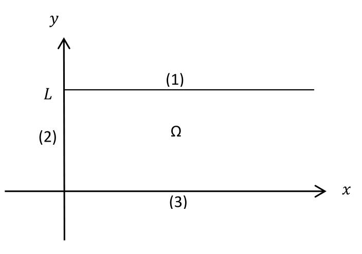 Figure 1
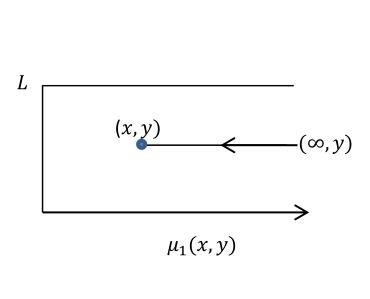 Figure 2
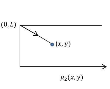 Figure 3
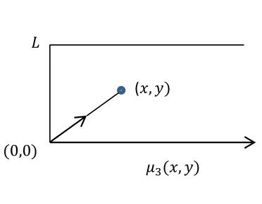 Figure 4
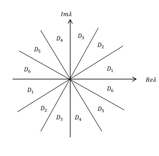 Figure 5
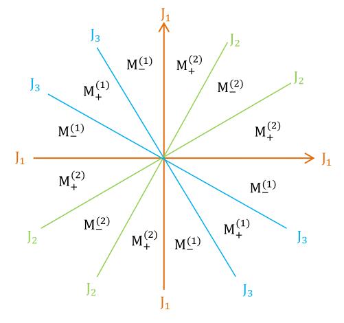 Figure 6
Peer Reviews
No public reviews on file for this paper yet. If you reviewed it on a platform where reviews are public (OpenReview, ICLR, NeurIPS, ICML), you can paste yours below so the community can read it here.
Videos
No videos yet. Explain this paper in a talk, walkthrough, or lecture? Add one.
00footnotetext: †: Corresponding author.
Email addresses : [email protected](N.Zhang); [email protected](T.c.Xia); [email protected](B.b.Hu)
A Riemann-Hilbert Approach to the Complex Sharma-Tasso-Olver Equation on the Half Line
**Ning Zhang †a,b,Tiecheng Xia a, Beibei Hua,c
a Department of Mathematics, Shanghai University, Shanghai, 200444, PR China
b Department of Basical Courses, Shandong University of Science and Technology, Taian 271019, PR China
c School of Mathematicas and Finance, Chuzhou University, Anhui, 239000, China**
Abstract: In this paper, we use the Fokas method to analyze the complex Sharma-Tasso-Olver(cSTO) equation on the half line . Assuming that the solution of the cSTO equation is exists, we show that it can be represented in terms of the solution of a matrix Riemann-Hilbert problem(RHP) formulated in the complex plane (the Fourier plane), which has a jump matrix with explicit dependence involving four scalar functions of , called spectral functions. The spectral functions and are obtained from the initial data and the boundary data , respectively. The problem has the jump across . The spectral functions are not independent, but related by a compatibility condition, the so-called global relation. Given initial and boundary values and such that there exist spectral functions satisfying the global relation, we show that the function defined by the above Riemann-Hilbert problem exists globally and solves the cSTO equation with the prescribed initial and boundary values.
Key word: Riemann-Hilbert problem; the cSTO equation; initial-boundary value problem; jump matrix
2010 MR Subject Classification 35G31; 35Q15
1 Introduction
A unified method for analyzing boundary value problems with decaying initial data, extending ideas of the so-called inverse scattering transform(IST) method, was discovered in 1967[1]. This method can be thought of as a nonlinear Fourier transform(FT) method. However, this nonlinear FT is not the same for every nonlinear evolution equation, but it is constructed from the part of the Lax pair. Furthermore, neither the direct nonlinear FT of the initial data, nor the inverse nonlinear FT can be expressed in closed form: the former involves a linear Volterra integral equation and the latter involves a matrix Riemann-Hilbert problem(RHP). The part is used only to determine the evolution of the direct nonlinear FT[2,3]. However, in many laboratory and field situations, the wave motion is initiated by what corresponds to the imposition of boundary conditions rather than initial conditions. This naturally leads to the formulation of an initial-boundary value (IBV) problem instead of a pure initial value problem.
In 1997, a new unified approach based on the Riemann-Hilbert factorization problem to solve IVB problems for linear and nonlinear integrable PDEs was presented by Fokas [4], we call that Fokas method. The Fokas method provides a generalization of the inverse scattering formalism from initial value to IVB problems, it is not only able to identify the linearizable class of boundary conditions, but what is more important, it is able to solve this class of boundary value problems as effectively as the usual class of initial value problems on the line. Over the last almost two decades, it was further developed by Its[5,6], de Monvel[7,8], Lenells[9-11], Engui Fan and JianXu[12-14] ect. After intense investigation it appears that there exists now an elegant, rigorous method for solving the half line problem for integrable nonlinear PDE s. An effort has been made to present this new method in a form that will be accessible to a wide audience. This is important, since it is hoped that researchers will consider using this method to solve a large class of physically important boundary value problems which remain open. Furthermore, it is interesting that this new method gives rise to a new numerical method for solving linear elliptic boundary value problems (this method is based on the numerical solution of the global relation [15]).
The Sharma-Tasso-Olver(STO) equation
[TABLE]
was first derived as an example of odd members of Burgers hierarchy by extending the ”linearization” achieved through the Cole-Hopf ansatz to equations containing as highest derivatives odd space derivatives[16]. In recent years, many physicists and mathematicians have paid much attention to the STO equation due to its importance in mathematical physics. The bi-Hamiltonian formulation and the generalized Poisson bracket are pre- sented in [17], the exact traveling solutions and symmetries of the STO equation were extensively studied in the literature[17-19]. Moreover, the multiple solitons, exact traveling solutions, kinks solutions, non-traveling wave solutions of the STO equation were obtained with different approaches[18-22]. In this paper, we concerned with the cSTO equation derived by Fan[23]
[TABLE]
If we let in the spectral problem (1.2), then we will get the real version of the STO equation (1.1). The purpose of this paper is to analyze the IBV problem for the cSTO equation (1.2) on the half line using Fokas method. That is, in the quarter plane
[TABLE]
where is a positive finite constant. The side , and will be referred to as side (1), (2) and (3), respectively, see Fig.1.
Assuming that the solution of the cSTO equation exists, define
[TABLE]
and
[TABLE]
We show that it can be represented in terms of the solution of a matrix RHP formulated in the plane of the complex spectral parameter . The jump matrix has explicit dependence and is given in terms of the spectral functions and , which are obtained from the initial data (1.4) and the boundary data (1.5), respectively. The problem has the jump across . The spectral functions are not independent, but related by a compatibility condition, the so-called global relation, which is an algebraic equation coupling and . An important advantage of the methodology of ref.[4] is that it yields precise information about the long time asymptotic of the solution. The usefulness of the asymptotic information for a physical problem can be understood by considering an example where the field is at rest at some initial time . Assuming that we can create or measure the waves emanating from some fixed point, say . In space, we arrive at an initial-boundary value problem for which the initial datum vanishes identically, while the boundary values , , are at our disposal. An analysis of the asymptotic behavior of the solution then provides information about the long time effect of the known boundary values. In Section 2, we give some summary results and the basic RHP of the cSTO equation (1.2). In Section 3, we construct the inverse spectral mappings for the initial and boundary values. In the following Section 4, the spectral functions and are investigated and the principal RHP is presented.
2 The Basic RHP of CSTO Equation
Frist, we explain what the RHP is.
Definition 2.1. Let the contour be the union of a finite number of smooth and oriented curves on the Riemann sphere , such that has only a finite number of connected components. Let be a matrix defined on the contour , the RHP is the problem of finding a matrix-valued function that satisfies
(i)
is analytic for all , and extends continuously to the contour ;
(ii)
;
(iii)
as .
**2.1.Lax pair for the cSTO equation
**The cSTO equation (1.2) admits the Lax pair[23]
[TABLE]
where
[TABLE]
and Indeed, one can check that the compatibility condition of the two equations in (2.1) yields the zero-curvature equation , which is exactly the cSTO equation (1.2). Here the square bracket is the usual matrix commutator defined as .
In what follows, rather than work with the original form of Lax pair(2.1), it turns out to be more convenient by introducing
[TABLE]
denotes the third Pauli’s matrix, we can rewrite the Lax pair (2.1) in a matrix form
[TABLE]
where . Extending the column vector to a matrix and letting
[TABLE]
Using Equ.(2.4), the original form of Lax pair (2.1) can be rewritten in the form
[TABLE]
which can be written in full derivative form
[TABLE]
where, denotes the matrix commutator with , , then can be easily computed ( is a matrix), , and .
Statement of the problem. Let satisfy a nonlinear evolution equation with spatial derivatives of order , on the half line , and for , where is a positive constant. Let satisfy decaying initial conditions at , as well as appropriate boundary conditions at . Assume that this PDE admits a Lax pair formulation of the type (2.5), i.e. assume that this PDE is equivalent to the compatibility condition of Eq.(2.2). Then such an initial-boundary value problem can be analyzed using the Fokas and Lenells method[10,14,24,25]. **2.2. Spectral Analysis and Asymptotic Analysis
**Consider that a solution of Eq.(2.5) is of the form
[TABLE]
where are independent of . Substituting the above expansion into the first equation of (2.5), and comparing the same order of frequency of , we have
[TABLE]
Let denotes the off-diagonal part of , denotes the diagonal part of , is a matrix. From (2.8) we have
[TABLE]
and
[TABLE]
where, is a diagonal matrix.
On the other hand, substituting the above expansion into the second equation of (2.5), we have
[TABLE]
From (2.11), we have
[TABLE]
and
[TABLE]
We note that the Eq.(1.2) admits the conservation law
[TABLE]
Then the two Eq.(2.10) and Eq.(2.13) for are consistent and are both satisfied if we define
[TABLE]
where is the closed real-valued one-form, and
[TABLE]
simultaneity, for the convenience of calculation we denote
**2.3. Eigenfunctions and Their Relations
**Noting that the integral in Eq.(2.15) is independent of the path of integration and the is independent of , then we can introduce eigenfunction as follows
[TABLE]
where is a matrix-valued function. Through direct calculation, the Lax pair of Eq.(2.6) becomes
[TABLE]
where
[TABLE]
[TABLE]
[TABLE]
and
[TABLE]
Then Eq.(2.19) for can be written as
[TABLE]
where
Assuming that exists and is sufficiently smooth in , are the matrix valued functions defined by
[TABLE]
The integral denotes a smooth curve from to , and .
The fundamental theorem of calculus implies that the functions satisfy Eq.(2.18). Since the one-form is exact, then are independent of the path of integration. We choose the particular contours shown in Fig.2.
This choice implies the following inequalities on the contours
[TABLE]
The functions , and are defined from in some domain of the complex -plane. Following the idea in Ref.[15], we have
[TABLE]
[TABLE]
[TABLE]
We find that the first column of the matrix Eq.(2.26) involves , the first column of the matrix Eq.(2.27) and Eq.(2.28) involve and . Using the above inequalities (2.25) implies that the exponential term of is bounded in the following regions of the complex -plane,
[TABLE]
where denote the the first column of the matrix . The second column of the matrix Eq.(2.26) involves the inverse of the above exponential, similar considerations are valid for . We have
[TABLE]
We define the in the complex -plane by
[TABLE]
where denotes the argument of the , see Fig.3.
Then, we obtain
[TABLE]
where denotes which is bounded and analytic for .
More specifically,
[TABLE]
**2.4. The Spectral Functions and Their Propositions
**The crucial advantage of requiring that the functions solve equation (2.24) is that any two such functions are related via a matrix that has explicit exponential dependence of the form , where the function can be computed by evaluating the relevant relation at any convenient point in the domain . In particular, using that . In order to deriving a RHP, we need to compute the jumps across the boundaries of the ’s . It turns out that the relevant jump matrices can be uniquely defined in terms of two matrices valued spectral functions and defined as follows
[TABLE]
Evaluating the first equation of (2.34) at and the second equation of (2.34) at , implies
[TABLE]
From Eq.(2.34) and Eq.(2.35), we obtain
[TABLE]
which will lead to the global relation.
Hence, the function can be obtained from the evaluations at of the function and can be obtained from the evaluations at of the function . And these functions about satisfy the linear integral equations as follows
[TABLE]
[TABLE]
[TABLE]
[TABLE]
Let , , and be the initial and boundary values of , then
[TABLE]
[TABLE]
where
[TABLE]
These expressions for contain only and , respectively. Therefore, the integral equation (2.37) determining is defined in terms of the initial data , the integral equation (2.40) determining is defined in terms of the initial data and .
Following the Section 2.4. of the Ref.[9], let us show the function satisfy the symmetry relations. The analytic properties of matrices that come from Eq.(2.26), Eq.(2.27) and Eq.(2.28) are collected in the following proposition. Setting
\mu_{j}(x,y;\lambda)=(\mu_{j}^{(1)}(x,y;\lambda),\mu_{j}^{(2)}(x,y;\lambda))=\left(\begin{array}[]{cc}\mu_{j}^{11}&\mu_{j}^{12}\\ \mu_{j}^{21}&\mu_{j}^{22}\\ \end{array}\right),j=1,2,3.
Proposition 2.4.1. The matrices have the following properties
(1)
;
(2)
is analytic, and ;
(3)
is analytic, and ;
(4)
is analytic, and ;
(5)
is analytic, and ;
(6)
is analytic, and ;
(7)
is analytic, and .
Proposition 2.4.2.(Symmetries) The matrices \mu_{j}(x,y;\lambda)=\left(\begin{array}[]{cc}\mu_{j}^{11}(x,y;\lambda)&\mu_{j}^{12}(x,y;\lambda)\\ \mu_{j}^{21}(x,y;\lambda)&\mu_{j}^{22}(x,y;\lambda)\\ \end{array}\right)(j=1,2,3.) have the following properties
(1)
, ;
(2)
, ,
, .
Proposition 2.4.3. The spectral function and are defined in Eq.(2.34) and Eq.(2.35) imply that
[TABLE]
If satisfies Eq.(2.3), it follows that is independent of and . Hence, since , the determinant of the function corresponding to according to (2.17) is also independent of and . In particular, for evaluation of at shows that and . According to Proposition 2.4.2, we can construct the following matrix spectral functions and ,
[TABLE]
By use of Eq.(2.35), we can obtain the proposition about the matrix spectral functions (2.44).
**Proposition 2.4.4.**The spectral function and are constructed in Eq.(2.44) have the following properties
- (1)
\left(\begin{array}[]{c}b(\lambda)\\ a(\lambda)\\ \end{array}\right)=\mu_{1}^{(2)}(0,0;\lambda)=\left(\begin{array}[]{c}\mu_{1}^{12}(0,0;\lambda)\\ \mu_{1}^{22}(0,0;\lambda)\\ \end{array}\right).\\
- (2)
\left(\begin{array}[]{c}-e^{-4i\lambda^{6}L}B(\lambda)\\ \overline{A(\bar{\lambda})}\\ \end{array}\right)=\mu_{3}^{(2)}(0,L;\lambda)=\left(\begin{array}[]{c}\mu_{3}^{12}(0,L;\lambda)\\ \mu_{3}^{22}(0,L;\lambda)\\ \end{array}\right).
- (3)
\partial_{x}\mu_{1}^{(2)}(x,0;\lambda)-2i\lambda^{2}\tilde{\sigma}\mu_{1}^{(2)}(x,0;\lambda)=N_{1}(x,0;\lambda)\mu_{1}^{(2)}(x,0;\lambda),\,\,\,\lambda\in D_{1}\bigcup D_{2}\bigcup D_{3},0<x<\infty,\\ \partial_{y}\mu_{3}^{(2)}(0,y;\lambda)+4i\lambda^{6}\tilde{\sigma}\mu_{3}^{(2)}(0,y;\lambda)=N_{2}(0,y;\lambda)\mu_{3}^{(2)}(0,y;\lambda),\,\,\,\lambda\in D_{2}\bigcup D_{4}\bigcup D_{6},0<y<L,\\ where\tilde{\sigma}=\left(\begin{array}[]{cc}1&0\\ 0&0\\ \end{array}\right).
- (4)
,, and obey the symmetries
- (5)
- (6)
, uniformly as with , uniformly as with
**2.5. The Global Relation
**Let and denote the eigenfunction obtained from the evaluation of and at , respectively
[TABLE]
The eigenfunctions and satisfy the differential Eq.(2.23) thus, they are simply related
[TABLE]
Evaluating this equation at , we obtain the global relation
[TABLE]
Remark 2.5.1. For the NLS, there exists one unknown boundary value. Thus, one might expect that since the global relation (2.24) provides one equation connecting this unknown function with the given initial and boundary conditions, in this case, it is possible, by utilizing the global relation, to characterize the unknown boundary value. However, for the mKdV, there exist two unknown boundary values. In this case, the solution of the associated linear problem suggests that it is impossible to solve this problem, unless one uses the transformation that leaves invariant in order to obtain an additional equation from the global relation.
Remark 2.5.2. It is important to note that the rigorous result mentioned earlier does not require the knowledge of the explicit form of , it only requires the existence of a function with specific analyticity properties. This suggests that the most efficient approach of characterizing is to actually eliminate . This is precisely the philosophy used in the linear limit for the derivation of the generalized Dirichlet to Neumann map and it is also the philosophy used in [5,8].
**2.6. The Basic RHP
**Following, according to the paper [16], we can get that the RHP of the cSTO equation. Equation (2.34) relating the various analytic eigenfunctions, can be rewritten in a form that determines the jump conditions of a RHP, with unitary jump matrices on the real and imaginary axis. This involves tedious but straight forward algebraic manipulations. The final form is
[TABLE]
where and have two forms of expression, respectivly
[TABLE]
Equation (2.46) imply that
[TABLE]
Setting , we have the following theorem
Theorem2.6.1. Let is a smooth function, are defined by Eq.(2.26), Eq.(2.27) and Eq.(2.28), be defined by Eq.(2.46), then satisfies the jump condition
[TABLE]
where
[TABLE]
[TABLE]
The contour for this RHP is depicted in Fig.4.
Proof. Using the idea in ref.[17], in order to derive the jump condition Eq.(2.47) we write Eq.(2.34) and Eq.(2.36) in the following form
[TABLE]
[TABLE]
[TABLE]
By direct calculation, we can derive that the jump matrices satisfy the jump condition Eq.(2.47).
Further more, we can obtain the jump condition between and
[TABLE]
where .
**2.7. The Residue Conditions.
**The matrix of this RHP is a sectionally meromorphic function of in . The possible poles of are generated by the zeros of , and by the complex conjugates of these zeros. Since , are even functions, this means each zero of is accompanied by another zero at . Similarly, each zero of is accompanied by a zero at . In particular, both and have even number of zeros.
**Hypothesis 2.7.1. ** We assume that
- •
has simple zeros(), such that ( ) lie in , and () lie in .
- •
has simple zeros(), such that (), lie in , and , , lie in .
- •
None of the zeros of coincides with any of the zeros of .
The residues of the function at the corresponding poles can be computed using Eq.(2.34) and Eq.(2.36). Using the notation for the first column and for the second column of the solution of the RHP, and we write , then we get the following proposition.
Proposition 2.7.2.
(1)
Res =, .
(2)
Res =, , .
(3)
Res =, .
(4)
Res =, .
Proof.
According to the idea in ref.[17], we only need to prove (1), and another three relations also have similar proof.
Consider , the simple zeros () of are the simple poles of . Then we have
[TABLE]
Taking into the second equation of Eq.(2.52) we obtain
[TABLE]
Furthermore,
[TABLE]
It is equivalent to Proposition 2.7.2(1).
3 Inverse Spectral Mappings
In this section we turn to the description of the inverse spectral mappings. They will be given in terms of the solutions of the associated RHP, the jump matrices of which are constructed from the corresponding spectral functions. The guideline for the choice of a particular configuration of these boundary RHP is that they must be conveniently related to the bulk RHP, to be constructed for the solution of the CSTO equation in the whole domain. Following this idea, we rewrite the jump condition Eq.(2.50)
[TABLE]
where . The asymptotic conditions of Eq.(2.26) Eq.(2.27) Eq.(2.28) and the Proposition 2.4.1 imply
[TABLE]
where . Eq.(3.1) and the condition Eq.(3.2) yield the following integral representation for the function
[TABLE]
then
[TABLE]
Using Eq.(3.2) and the ODE of the Lax pair (2.5), we find
[TABLE]
[TABLE]
where denote the usual Pauli matrix and \sigma_{1}=\left(\begin{array}[]{cc}0&1\\ 1&0\\ \end{array}\right).
The inverse problem involves reconstructing the potential from the spectral functions , That means we will reconstruct the potential . We show in Section 2.2 that
[TABLE]
when
[TABLE]
is a solution of Eq.(2.5). This implies that
[TABLE]
where
[TABLE]
is the corresponding solution of Eq.(2.18) related to via Eq.(2.18), and we write for . From Eq.(3.7) and its complex conjugate , we obtain
[TABLE]
Then we can solve the inverse problem as follows
(1)
Use any one of the three spectral functions to compute according to
[TABLE]
(2)
Determine from Eq.(2.16).
(3)
Finally, is given by Eq.(3.7).
4 The Spectral Functions and the principal RHP
**4.1.The spectral functions
**The analysis of Section 2 motivates the following definitions for the spectral functions.
Definition 4.1.1. (The spectral functions and Given the smooth function , we define the map
[TABLE]
by
[TABLE]
where is the unique solution of the Volterra linear integral equation
[TABLE]
and is given in terms of by Eq.(2.41). The spectral functions and have the same properties with Proposition 2.4.4.
Definition 4.1.2. We define is the inverse map of ,
[TABLE]
where Theorem 4.1.3
- •
is the unique solution of the following RHP
M^{(x)}(x,\lambda)=\left\{\begin{array}[]{ll}M_{-}^{(x)}(x,\lambda),&Im\lambda^{2}<0\\ M_{+}^{(x)}(x,\lambda),&Im\lambda^{2}>0\end{array}\right. is a sectionally meromorphic function, then satisfied the jump condition
[TABLE]
where
[TABLE]
and satisfy asymptotic properties
- •
We assume that the spectral function has simple zeros(), such that, () lie in , () lie in . The first column of has simple poles at , , the second column of has simple poles at , . The associated residues are given by
[TABLE]
[TABLE]
Proof. We note that and have the following forms,
[TABLE]
According to Eq.(2.52), we only need to set ,
[TABLE]
by direct calculation, we can derive that the jump matrices (Eq.(4.5)) satisfy the jump condition Eq.(4.4).
Consider the second column of , the simple zeros () of are the simple poles of . Then we have
[TABLE]
Taking into the second equation of Eq.(4.8) we obtain
[TABLE]
Furthermore,
[TABLE]
It is equivalent to Eq.(4.6) and using the same proof method we can derive out Eq.(4.7).
**4.2.The spectral functions
Definition 4.2.1.** Let , and be smooth functions, we define the map
[TABLE]
by
[TABLE]
where is the unique solution of the Volterra linear integral equation
[TABLE]
and is given by Eq.(2.42). The spectral functions and have the same properties with Proposition 2.4.4.
Definition 4.2.2. We define is the inverse map of ,
[TABLE]
where
[TABLE]
[TABLE]
[TABLE]
where the functions are determined by the asymptotic expansion Eq.(4.21), and is the unique solution of the RHP in the following Theorem 4.2.3.
Theorem 4.2.3
- •
is the unique solution of the following RHP,
M^{(y)}(y,\lambda)=\left\{\begin{array}[]{ll}M_{-}^{(y)}(y,\lambda),&Im\lambda^{6}<0\\ M_{+}^{(y)}(y,\lambda),&Im\lambda^{6}>0\end{array}\right. is a sectionally meromorphic function, then satisfied the jump condition
[TABLE]
where,
[TABLE]
and satisfy asymptotic properties
[TABLE]
- •
We assume that the spectral function has simple zeros(), such that, () lie in , () lie in . The first column of has simple poles at , , the second column of has simple poles at , . Then, the associated residues are given by
[TABLE]
[TABLE]
Proof. We set
[TABLE]
In order to obtain the jump matrix , we set according to Eq.(2.52),
[TABLE]
by direct calculation, we can derive that the jump matrices (Eq.(4.20)) satisfy the jump condition.
Consider the first column of , the simple zeros () of are the simple poles of . Then we have
[TABLE]
Taking into the second equation of Eq.(4.25) we obtain
[TABLE]
Furthermore,
[TABLE]
It is equivalent to Eq.(4.22) and using the same proof method we can derive out Eq.(4.23).
**4.3.The spectral functions
Definition 4.3.1.**Given the spectral functions
[TABLE]
and the smooth functions . We define the map
[TABLE]
by
[TABLE]
where is the unique solution of the Volterra linear integral equation and , is given by
[TABLE]
Proposition 4.3.2. The spectral functions and have the following properties
(i)
and are analytic for and continuous and bounded for ;
(ii)
as , ;
(iii)
, ;
(iv)
, .
Definition 4.3.3. We define is the inverse map of ,
[TABLE]
where Theorem 4.3.4
- •
is the unique solution of the following RHP
M^{(L)}(x,\lambda)=\left\{\begin{array}[]{ll}M_{-}^{(L)}(x,\lambda),&Im\lambda^{2}<0\\ M_{+}^{(L)}(x,\lambda),&Im\lambda^{2}>0\end{array}\right. is a sectionally meromorphic function, then satisfied the jump condition
[TABLE]
where
[TABLE]
and satisfy asymptotic properties
- •
We assume that the spectral function has simple zeros(), such that, () lie in , () lie in . The second column of has simple poles at , , the first column of has simple poles at , . The associated residues are given by
[TABLE]
[TABLE]
Proof. We note that and have the following forms,
[TABLE]
According to Eq.(2.54), we only need to set ,
[TABLE]
by direct calculation, we can derive that the jump matrices (Eq.(4.34)) satisfy the jump condition Eq.(4.33).
Consider the frist column of , the simple zeros () of are the simple poles of . Then we have
[TABLE]
Taking into the second equation of Eq.(4.38) we obtain
[TABLE]
Furthermore,
[TABLE]
It is equivalent to Eq.(4.35) and using the same proof method we can derive out Eq.(4.36).
**4.4. The principal RHP
Theorem 4.4.1.** Let is a smooth function. Suppose that the function are compatible with the function at . Define the spectral function , , and , in terms of , , and of Definition 4.1.2 and Definition 4.2.2. Suppose that , , and satisfy the global relation
[TABLE]
where , if the global relation is replaced by . Assume that the possible zeros of are and of , then define the as the solution of the following RHP
- •
is sectionally meromorphic in .
- •
The first column of has simple poles at , , and , . The second column of has simple poles at , , and , .
- •
satisfies the jump condition
[TABLE]
- •
.
- •
satisfies the residue conditions of Proposition2.7.2.
Then exists and is unique, we define in terms of by
[TABLE]
Furthermore is the solution of the cSTO equation (1), and , , , .
Proof. In fact, if we assume that and have no zeroes, then the function satisfies a non-sigular RHP. Using the fact that the jump matrix matches with the symmetry conditions, we can show that this problem has a unique global solution [26]. The case that and have a finite number of zeros can be mapped to the case of no zeros supplemented by an algebraic system of equations which is always uniquely solvable.
Theorem 4.2.2. The RHP inTheorem 4.2.1 with the vanishing boundary condition (, has only the zero solution.
Proof. Assume that is a solution of the RHP in Theorem 4.2.1 such that (. is a matrix, denotes the complex conjugate transpose of .
Define
[TABLE]
where the and are dependence. and are analytic in and respectively. By the symmetry relations and and Eq.(31), we infer that
[TABLE]
Then
[TABLE]
Eq.(4.45) and Eq.(4.46) mean that for . Therefore, and define an entire function vanishing at infinity, so and are identically zero. Noting is a Hermitian matrix with unit determinant and entry for any . Therefore, is a positive definite matrix. Since vanishes identically for , i.e.
[TABLE]
We can deduce that as . It follows that and vanish identically.
Proposition 4.2.3. **Proof that satisfies the cSTO equation.
**Using arguments of the dressing methods[19], it can be verified directly that if is defined as the unique solution of the above RHP, and if is defined in terms of by Eq.(4.43), then and satisfy two parts of the Lax pair, hence is solvable on cSTO equation.
5 Acknowledgments
This work is in part supported by the National Natural Science Foundation of China( NNSFC Grant Nos. 11271008, 61072147).
Reference
[1] Gardner G.S., Greene, J.M., Kruskal, M.D., Miura, R.M.: Phys. Rev. Lett. 19, 1095 (1967).
[2] Faddeev L.D., Takhtajan, L.A.: Hamiltonian Methods in the Theory of Solitons. Berlin-Heidelberg-NewYork: Springer Verlag, 1987.
[3] Fokas A.S., Zakharov, V.E. (eds): Important Developments in Soliton Theory. Berlin-Heidelberg-NewYork: Springer Verlag, 1994.
[4] Fokas A.S. A unified transform method for solving linear and certain nonlinear PDEs. Proc R Soc Lond A, 1997, 453: 1411-1443.
[5] Fokas A.S, Its A R, Sung L Y. The nonlinear Schr?dinger equation on the half-line. Nonlinearity, 2005, 18:1771-1822.
[6] Its, Alexander, Shepelsky, Dmitry. Initial boundary value problem for the focusing nonlinear Schrödinger equation with Robin boundary condition: half-line approach. Proc. R. Soc. Lond. Ser. A Math. Phys. Eng. Sci. 469 (2013), no. 2149, 20120199, 14 pp.
[7]Boutet de Monvel A, Fokas A.S, Shepelsky D. The mKDV equation on the half-line. J Inst Math Jussieu, 2004, 3: 139-164.
[8] Boutet de Monvel A, Shepelsky D. Initial boundary value problem for the MKdV equation on a finite interval. Ann Inst Fourier (Grenoble), 2004, 54: 1477-1495.
[9] Lenells Jonatan, The derivative nonlinear Schrödinger equation on the half-line. Physica D 2008, 237: 3008 C3019.
[10]Lenells Jonatan, An integrable generalization of the sine-Gordon equation on the half-line. IMA J. Appl. Math. 76 (2011), no. 4, 554-572.
[11] Lenells, Jonatan, The nonlinear steepest descent method: asymptotics for initial-boundary value problems. SIAM J. Math. Anal. 48 (2016), no. 3, 2076-2118.
[12] Xu Jian, Fan Engui, The unified transform method for the Sasa-Satsuma equation on the half-line. Proc. R. Soc. Lond. Ser. A Math. Phys. Eng. Sci.469, no.2159, 20130068, (2013)35-55.
[13] Xu Jian, Fan Engui, The three-wave equation on the half-line. Phys. Lett. A 378 (2014), no. 1-2, 26-33.
[14] Xu Jian, Fan Engui, Initial-boundary value problem for integrable nonlinear evolution equation with Lax pairs on the interval. Stud. Appl. Math. 136 (2016), no. 3, 321-354.
[15] Fulton, S.R., Fokas, A.S., Xenophontos, C.A. An analytical method for linear elliptic PDEs and its numerical implementation. J. Comput. Appl. Math. 167 (2004), no. 2, 465-483.
[16] H. Tasso, Coles ansatz and extension of Burgers equation, Report No. IPP6/142 (Ber. MPI fur Plasma physik, Garching,1976).
[17] H. Tasso, Hamiltonian formulation of odd Burgers hierarchy, J. Phys. A. 29 (1996) 7779-7784.
[18] F. Verheest, W. Hereman, Nonlinear mode decoupling for classes of evolution equations, J.Phys. A. 15 (1982) 95-102.
[19] Wang, Deng-Shan; Yin, Shujuan; Tian, Ye; Liu, Yifang Integrability and bright soliton solutions to the coupled nonlinear Schr?dinger equation with higher-order effects. Appl. Math. Comput. 229 (2014), 296 C309.
[20] Dong Huan He; Guo Bao Yong; Yin Bao Shu; Generalized Fractional Supertrace Identity For Hamiltonian Structure of Nls-Mkdv Hierarchy With Self-Consistent Sources. Analysis and Mathematical Physics,6,2,199-209,2016.
[21] V. V. Gudkov, A family of exact traveling wave solutions to nonlinear evolution and wave equations, J. Phys. A 38(9),4794-4803 (1997).
[22]Chao Yue, Tiecheng Xia, Algebro-geometric solutions for the complex Sharma-Tasso-Olver hierarchy, Journal of Mathematical Physics 55, 083511 (2014).
[23] Fan Engui, A family of completely integrable multi-Hamiltonian systems explicitly related to some celebrated equations, J. Math. Phys. 42(9), 4327-4344 (2001).
[24] Fokas, A.S., Lenells, J., The unified transform for the modified Helmholtz equation in the exterior of a square. Unified transform for boundary value problems, 172 C180, SIAM, Philadelphia, PA, 2015.
[25] Fokas, A.S., Lenells, J., Pelloni, B. Boundary value problems for the elliptic sine-Gordon equation in a semi-strip. J. Nonlinear Sci. 23 (2013), no. 2, 241 C282.
[26] V.E.Adler, I.T.Khabibullin, Boundary conditions for integrable chains.(Russian) Funktsional. Anal.i Prilozhen. 31 (1997), no.2, 1-14, 95; translation in Funct.Anal.Appl. 31 (1997), no.2,75-85.