On structure-preserving model reduction for damped wave propagation in transport networks
Herbert Egger, Thomas Kugler, Bj\"orn Liljegren-Sailer and, Nicole Marheineke, Volker Mehrmann

TL;DR
This paper develops structure-preserving model reduction techniques for damped wave equations in pipeline networks, ensuring key physical properties are maintained during discretization and reduction, with practical algorithms based on Krylov subspaces.
Contribution
It introduces a novel structure-preserving Galerkin projection combined with Krylov subspace methods for model reduction of PDE-DAE systems in pipeline networks.
Findings
Reduced models preserve energy dissipation and passivity.
Algorithms ensure well-posedness and stability of reduced systems.
Numerical tests confirm the effectiveness of the proposed methods.
Abstract
We consider the discretization and subsequent model reduction of a system of partial differential-algebraic equations describing the propagation of pressure waves in a pipeline network. Important properties like conservation of mass, dissipation of energy, passivity, existence of steady states, and exponential stability can be preserved by an appropriate semi-discretization in space via a mixed finite element method and also during the further dimension reduction by structure preserving Galerkin projection which is the main focus of this paper. Krylov subspace methods are employed for the construciton of the reduced models and we discuss modifications needed to satisfy certain algebraic compatibility conditions; these are required to ensure the well-posedness of the reduced models and the preservation of the key properties. Our analysis is based on the underlying infinite dimensional…
Click any figure to enlarge with its caption.
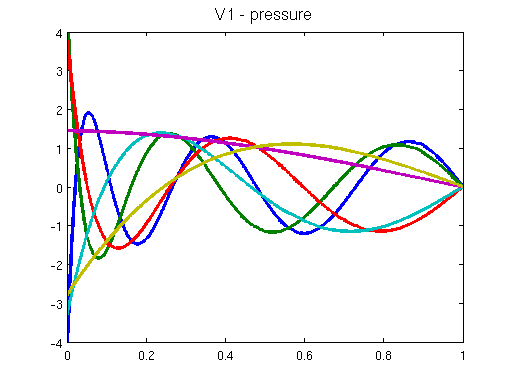 Figure 1
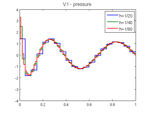 Figure 2
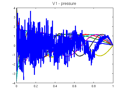 Figure 3
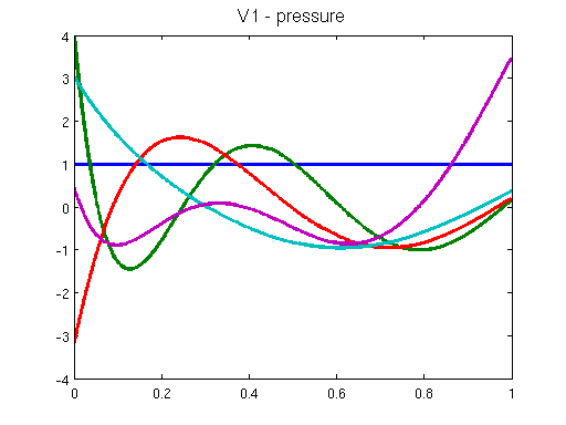 Figure 4
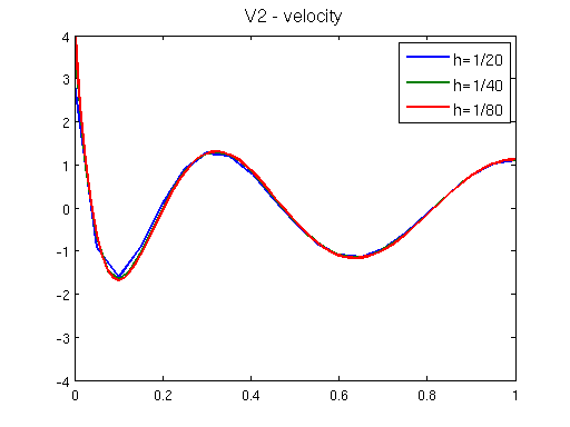 Figure 5
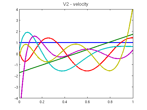 Figure 6
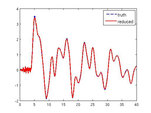 Figure 7
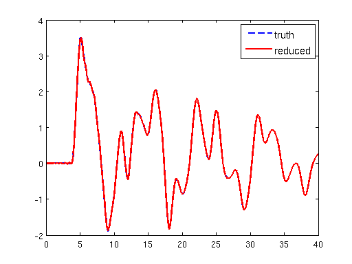 Figure 8
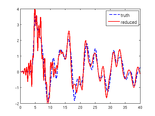 Figure 9
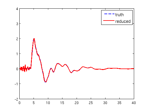 Figure 10
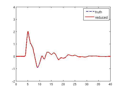 Figure 11
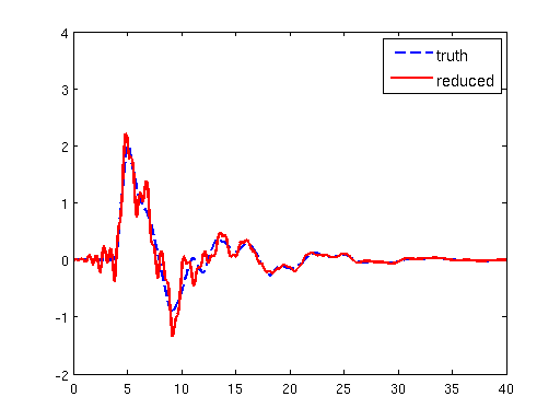 Figure 12
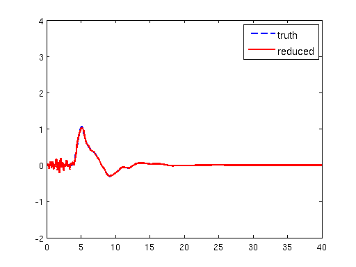 Figure 13
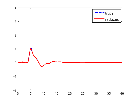 Figure 14
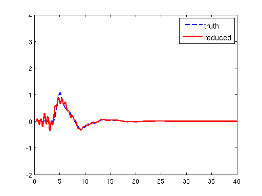 Figure 15
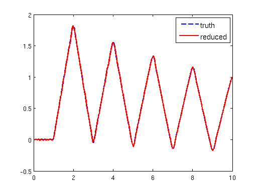 Figure 16
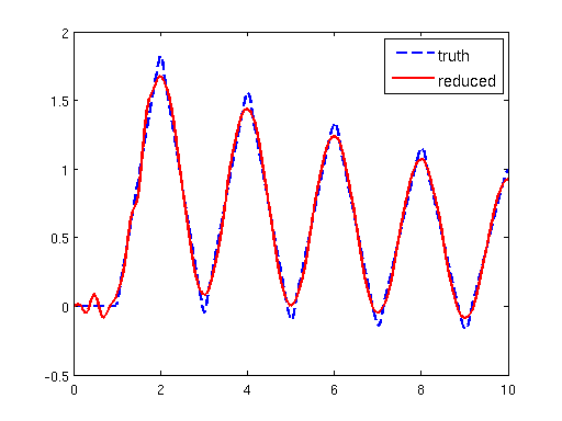 Figure 17
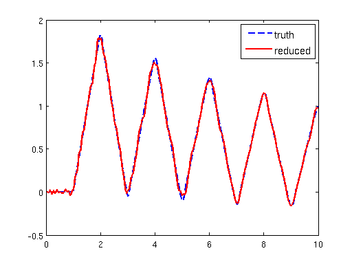 Figure 18
 Figure 19
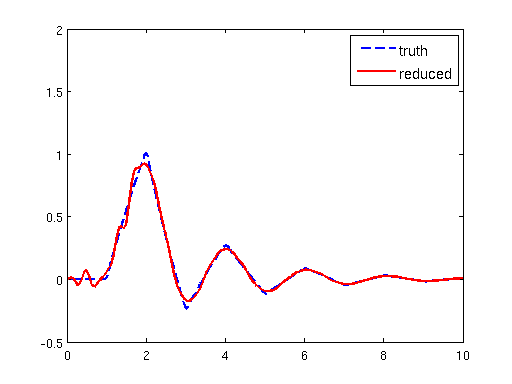 Figure 20
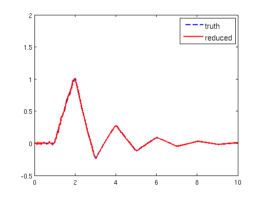 Figure 21
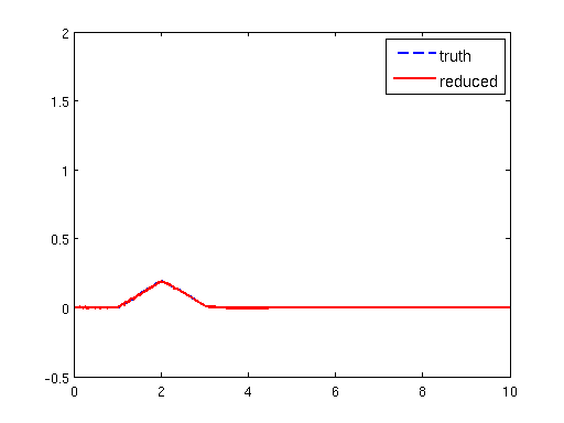 Figure 22
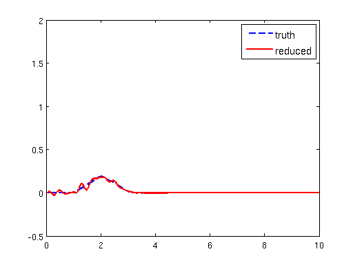 Figure 23
 Figure 24
| exact | ||||||||
| projection | ||||||||
| mass constraint | ||||||||
| exact | |||||||
|---|---|---|---|---|---|---|---|
Peer Reviews
No public reviews on file for this paper yet. If you reviewed it on a platform where reviews are public (OpenReview, ICLR, NeurIPS, ICML), you can paste yours below so the community can read it here.
Videos
No videos yet. Explain this paper in a talk, walkthrough, or lecture? Add one.
Taxonomy
TopicsNumerical methods for differential equations · Model Reduction and Neural Networks · Electromagnetic Simulation and Numerical Methods
On structure-preserving model reduction
for damped wave propagation in transport networks
H. Egger∗, T. Kugler∗, B. Liljegren-Sailer*†, N. Marheineke†*, and V. Mehrmann+
∗Department of Mathematics, TU Darmstadt
*†*Department of Mathematics, University Erlangen
+Inst. f. Mathematik, MA 4-5, TU Berlin, D-10623 Berlin
Abstract.
We consider the discretization and subsequent model reduction of a system of partial differential-algebraic equations describing the propagation of pressure waves in a pipeline network. Important properties like conservation of mass, dissipation of energy, passivity, existence of steady states, and exponential stability can be preserved by an appropriate semi-discretization in space via a mixed finite element method and also during the further dimension reduction by structure preserving Galerkin projection which is the main focus of this paper. Krylov subspace methods are employed for the construciton of the reduced models and we discuss modifications needed to satisfy certain algebraic compatibility conditions; these are required to ensure the well-posedness of the reduced models and the preservation of the key properties. Our analysis is based on the underlying infinite dimensional problem and its Galerkin approximations. The proposed algorithms therefore have a direct interpretation in function spaces; in principle, they are even applicable directly to the original system of partial differential-algebraic equations while the intermediate discretization by finite elements is only required for the actual computations. The performance of the proposed methods is illustrated with numerical tests and the necessity for the compatibility conditions is demonstrated by examples.
**Keywords: partial differential-algebraic equations, port-Hamiltonian systems, Galerkin projection, structure-preserving model reduction, passivity, exponential stability **
**AMS-classification (2000): 35L05, 35L50, 65L20, 65L80, 65F25, 65M60 **
1. Introduction
We study a system of partial differential-algebraic equations modeling the propagation of pressure waves in a pipeline network. The basic features of this problem are conservation of mass and dissipation of energy by friction which in turn yields passivity and exponential stability of the system and the convergence to unique steady states. All these properties can be preserved for an appropriate semi-discretization in space by mixed finite elements resulting in a finite dimensional differential-algebraic system with a port-Hamiltonian structure [17]. In this paper, we consider a further dimension reduction of these high dimensional models by structure-preserving Galerkin projection with the aim to obtain reduced models of smaller dimension which can be used for online simulation and control. These models should also yield a good approximation of the overall behavior and preserve the port-Hamiltonian structure and further relevant properties.
The model reduction of structured linear time-invariant systems has attracted significant interest in the literature, see e.g. [4, 20, 33, 35, 36, 41] and the references given there. Related results for second order systems have been obtained in [5, 6, 13, 38, 34], and the reduction of differential-algebraic equations has, for instance, been addressed in [3, 32]. Let us refer to [1, 9] for a general introduction to reduced order modeling and further references.
It is well-known that the port-Hamiltonian structure and thus passivity of the underlying system are inherited automatically by reduced models obtained via structure-preserving Galerkin projection [24, 37, 39]. The preservation of further properties, like conservation of mass or uniform exponential stability, however, requires the bases of the reduced models to satisfy additional compatibility conditions which have to be guaranteed explicitly.
The reduction of infinite dimensional systems described by partial differential or partial differential-algebraic equations has been considered, e.g., in [14, 26, 27], and in [23] the reduction of models arising in gas transport networks has been discussed. For such problems, or discretizations thereof, the bases for the reduced models have to be generated by some iterative process. Krylov subspace methods [2, 19, 22, 37] and proper orthogonal decomposition [14, 26, 27] are frequently employed for this purpose, and their analysis in a function space setting allows to obtain mesh independent results.
In this paper we consider a structure-preserving model reduction for large scale differential-algebraic systems obtained by discretization of a partial differential-algebraic model. We utilize Krylov subspace methods for the basis construction together with a structure-preserving space splitting and discuss appropriate modifications in order to satisfy some compatibility conditions required for the proof of mass conservation, uniform exponential stability, and the existence of steady states. While our algorithms are formulated in an algebraic setting, they also have an interpretation in function spaces. This is used already for the formulation of our algorithms and allows a complete analysis of the reduced models. Our methods therefore turn out to be almost independent of the intermediate finite element approximation used in computations and they are applicable, in principle, even directly to the underlying partial differential-algebraic system.
The outline of the paper is as follows: In the following section, we introduce the model problem under consideration and discuss the basic steps and arguments of our approach. The remainder of the manuscript is then split into three major parts: Part I is concerned with an outline and a partial analysis of the model reduction approach and Part II provides numerical illustration of these results. Part III contains the full analysis of the reduced order models obtained with our approach which requires us to consider the infinite dimensional problem and its approximation by mixed finite elements. The corresponding results mostly follow from those in [17] and they are therefore presented in the appendix for completeness and convenience of the reader.
2. Model problem and outline of the approach
The purpose of this section is to introduce in detail the problem under consideration and to give a rough idea of our approach and of the mutual relations between the underlying infinite dimensional system, the large scale finite dimensional systems arising after discretization in space, and the reduced models we are looking for.
2.1. Model problem
We consider the propagation of pressure waves in a one-dimensional network of pipes whose geometry shall be given as finite directed and connected graph with vertices and edges . On every pipe , the conservation of mass and the balance of momentum are described by
[TABLE]
Here , denote the pressure and mass flux which are functions of space and time, the coefficients , encode properties of the fluid and the pipe, and models the damping due to friction at the pipe walls. The coefficients are assumed to be positive and, for ease of presentation, constant on every pipe . At every inner vertex of the graph, corresponding to a junction of several pipes , we require that
[TABLE]
Here , depending on whether the pipe starts or ends at the vertex ; see Figure 2.1. Furthermore, , denote the respective functions evaluated at the vertex but still depending on time.
These coupling conditions model the conservation of mass and momentum at the junctions. At the boundary vertices , which correspond to the the ports of the network, we set
[TABLE]
with values denoting the given input at the port . As corresponding output of the system, we consider the mass flux via the ports, given by
[TABLE]
Other input and output configurations could be considered without difficulty as well. The specification of the model is completed by assuming knowledge of the initial conditions
[TABLE]
The system (2.1)–(2.7) models the propagation of pressure waves in a gas network on the acoustic time scale [12]. For sufficiently smooth initial data , , and appropriate compatible input functions , existence of a unique classical solution can be established [17].
2.2. Basic properties
The partial differential-algebraic system (2.1)–(2.5) encodes several interesting properties which are directly related to the underlying physical principles:
(P1) global conservation of mass, which here can be expressed as
[TABLE]
The total mass of the gas contained in the system can thus only be altered by flow of gas into or out of the system via the ports of the network.
(P2) a port-Hamiltonian structure, leading to energy dissipation and passivity, i.e.,
[TABLE]
The total energy in the system only changes by dissipation through damping and injection or extraction via the system ports. Apart from these basic properties, the system further admits
(P3) exponential stability and convergence to equilibrium for input ; more precisely,
[TABLE]
with constants and that are independent of the particular solution. For constant input , one can thus observe exponential convergence to
(P4) unique steady states for the corresponding stationary problem.
For a proof of these properties, let us refer to the appendix and to [17]. Systems of similar structure and with similar properties also model networks of electric transmission lines, vibrations of elastic multi-structures, or more general wave phenomena on multiply connected domains. Our arguments therefore may be useful in a wider context; see [9, 23, 30, 40] for further applications.
2.3. Full order model
An appropriate discretization of the partial differential-algebraic system in space by mixed finite elements leads to a differential-algebraic system
[TABLE]
which we will call the full order model in the sequel. In the context of reduced basis methods, the notion truth approximation is sometimes used instead. The vectors and are the algebraic representations of the states and after discretization, and resembles the Lagrange multiplier for the constraint (2.3). The output of the system is then given by
[TABLE]
If an appropriate discretization is used, the system matrices can be shown to have some basic structural properties. For ease of presentation, we formulate them here as assumptions:
- (A0)
, , are symmetric and positive definite and has trivial null-space.
The latter condition is equivalent to requiring that and the restriction of to the nullspace of define surjective linear operators.
Remark 2.1** (Notation).**
Throughout the paper, we identify matrices with corresponding linear operators. We call a matrix injective or surjective, if the operator has the respective property, and we write and for the range and the kernel of the corresponding operator. Furthermore denotes the image of the space under the map induced by .
Remark 2.2**.**
The differential-algebraic system (2.8)–(2.10) can be shown to formally have differentiation-index two [10, 29]. The condition that is injective, and hence that is surjective, however, allows to eliminate the Lagrange multiplier by purely algebraic manipulations and hence to reduce the system to an ordinary differential equation; see Section 6.2 and also refer to [8, 18, 25] for more general situations. Let us emphasize that the number of constraints amounts to the number of junctions in the network and thus is finite here.
Remark 2.3**.**
The system (2.8)–(2.10) can be written as linear time-invariant descriptor system
[TABLE]
From the particular form of the matrices and one can directly deduce the port-Hamiltonian structure, i.e., is symmetric and positive semi-definite and can be decomposed into an skew-symmetric part and a symmetric positive semi-definite part . This immediately guarantees the passivity of the system and further useful properties [42, 43].
The mass and the energy of the semi-discrete system (2.8)–(2.10) can be expressed as
[TABLE]
where is the vector representing the constant one function on the network. The basic properties (P1)–(P4) can then be shown to hold almost verbatim also for the semi-discrete problem which may therefore serve as a replacement for the infinite dimensional partial differential-algebraic problem under investigation.
2.4. Structure preserving model reduction
The main focus of the current paper is a further dimension reduction of the differential-algebraic model (2.8)–(2.10) by structure-preserving Galerkin projection of the following form: Given projection matrices of appropriate size and full rank, we set , , , , and . The reduced model is then defined as
[TABLE]
The tuple is the approximation for the exact solution of the full order model and serves as approximation for the output of the full system.
Remark 2.4**.**
Note that the dimension of the space for the Lagrange multiplier has not been reduced in the above construction; the network topology is thus completely maintained. The reduced model can again be written in the form of a descriptor system
[TABLE]
It is well-known [24, 37, 39] and easy to see for the system considered here that the port-Hamiltonian structure and thus passivity are inherited automatically by this kind of Galerkin projection. Additional conditions will, however, be required to establish the well-posedness of the resulting reduced differential-algebraic system and to characterize its index; see Section 3.3.
Similar as before, we will denote by
[TABLE]
the mass and energy of the reduced problem (2.14)–(2.16). An appropriate vector representing the constant one function on the network will be needed and additional compatibility conditions will be required to ensure well-posedness of the reduced system and the validity of (P1)–(P4).
2.5. Algebraic compatibility conditions
As we will demonstrate by explicit examples below, the validity of some of the properties (P1)–(P4) and even the well-posedness of the reduced models can in general not be guaranteed, unless additional assumptions on the projection matrices are satisfied. We will therefore require that
- (A1)
;
- (A2)
;
- (A3)
and .
Recall that and denote the range and the nullspace of the linear operator induced by a matrix and is the the image of the space under mapping induced by . Further, here denotes the identity matrix for the third component and is the vector used to describe the total mass of the full order system (2.8)–(2.10).
Remark 2.5**.**
Assumption (A1) will allow us to prove the conservation of mass also for the reduced models. The conditions (A2)–(A3), on the other hand, allow us to show that
- ()
, , and are symmetric and positive definite and has trivial nullspace;
see Lemma 3.4 for details. The reduced system thus has the same algebraic properties as the full order model (2.8)–(2.10). The well-posedness of the reduced system (2.14)–(2.16) can therefore be obtained with similar arguments as that of the full order model. The differentiation-index of the reduced model is again two and, by elimination of the Lagrange multiplier, we can obtain a regular system of ordinary differential equations; see Section 6.2 for details.
2.6. Basis construction
For the actual construction of the projection matrices , we consider an extension of the approach proposed in [20] together with some modifications in order to satisfy the compatibility conditions (A1)–(A3). The main steps can be sketched as follows:
- •
Krylov iteration: construct finite dimensional subspaces with good approximation properties by a Krylov iteration applied to the full order model (2.8)–(2.10).
- •
Splitting: Decompose as according to the components of the state .
- •
Modification: choose appropriate subspaces and and define
[TABLE]
such that the properties (A1)–(A3) can be verified for any choice of , , whose columns form bases for the corresponding subspaces.
With similar arguments as in [20], the reduced models (2.14)–(2.16) can be shown to match certain moments of the transfer function and thus to have good approximation properties. By construction, the projection matrices also satisfy the compatibility conditions (A1)–(A3). This will allow us to show that the reduced models are well-posed and that they inherit the structural properties (P1)–(P4) from the full order model.
2.7. Overview
The derivation of the properties (A0) for the system matrices of the full order model and of the algebraic compatibility conditions (A1)–(A3), as well as the complete analysis of the resulting reduced order models require us to consider in detail the connection between
- •
the underlying partial differential-algebraic equations;
- •
their discretization by Galerkin approximations in a function space setting; and
- •
the corresponding linear time-invariant systems in algebraic form.
A sketch of these different viewpoints is depicted in Figure 2.2. The close relation of the differential-algebraic systems to the problem on the continuous level will allow us to establish properties of the reduced order models that are uniform and almost independent of the intermediate full order model which is only required for the actual computations.
Apart from these analytical considerations, we also investigate in detail the algorithms for the actual subspace construction on the algebraic level and we address the following issues:
- •
The splitting step in the subspace construction turns out to be sensitive to numerical errors. To overcome this, we utilize a cosine-sine decomposition in the final algorithm.
- •
Round-off errors affect the validity of (A2) after the modification step outlined above. We therefore take special care in the basis construction to satisfy (A2) explicitly.
In order to reflect the functional analytic setting of the underlying infinite dimensional problem, we will utilize appropriate scalar products in the formulation of our algorithms on the algebraic level; see [27, 28] for similar approaches. As a consequence, the vectors obtained in the basis construction process can be interpreted as functions on the continuous level which allows for a further evaluation and interpretation of the numerical results.
Part I: Model reduction
In the following two sections, we present our model reduction approach on the algebraic level. We discuss in detail the construction of the reduced models and investigate their approximation properties. Futhermore, we address some algorithmic details.
3. Structure preserving model reduction
Let us first recall some basic facts about model order reduction and then informally discuss the algebraic compatibility conditions which are at the core of our model reduction approach. The basis construction algorithms on the algebraic level will then be presented in the next section.
3.1. Model reduction basics
Consider a general linear time-invariant descriptor system
[TABLE]
where , , are given matrices, symmetric and positive semi-definite, and defines a regular matrix pencil, i.e., is regular for almost every ; see [10, 15, 29, 31] for details. A formal expansion of the transfer function of the system [1, 9] leads to
[TABLE]
here is some given shift parameter. It is not difficult to see that the generalized moments can be written as with vectors that can be computed recursively by
[TABLE]
Let us denote by the th Krylov subspace generated by this iteration.
For any given projection matrix of appropriate dimension and maximal rank, we define , , and , and consider the reduced system
[TABLE]
resulting from Galerkin projection of (3.1) onto the range of the matrix . The transfer function of this reduced model may again be expanded as
[TABLE]
and the relation between the full and the reduced order model can be characterized as follows.
Lemma 3.1** (Moment matching).**
Let . Then for .
A proof of this assertion and further results can be found in [1, 9, 22]. The lemma can be interpreted as an abstract approximation result and may therefore serve as a quality indicator.
3.2. Basic properties of the full order model
The system (2.8)–(2.10) can be written in the compact form (3.1) with state vector and with system matrices defined by
[TABLE]
and under basic structural assumptions, the system (3.1) can be shown to be well-posed.
Lemma 3.2**.**
Let (A0) hold and let and be defined as above. Then defines a regular matrix pencil. Moreover, is regular for any and, in particular, is regular.
Proof.
First consider the case and set . We show that implies . Multiplication with from the left yields
[TABLE]
Since and are positive definite, this implies that and . But then
[TABLE]
From the assumptions on and , we can deduce the injectivity of , and hence .
Now consider the case : By simple rearrangement of the blocks of the matrix , we obtain
[TABLE]
Such a system is regular, if, and only if, is regular and has trivial nullspace; see [11] for the corresponding result in infinite dimensions. These properties are guaranteed by assumption (A0), which yields the invertibility of and hence also of . ∎
Remark 3.3**.**
Only the injectivity of , or equivalently, the surjectivity of is required to obtain a regular matrix pencil for and thus to establish well-posedness for the time-dependent problem. The stronger condition that is injective is, however, necessary to obtain regularity of the matrix and thus to ensure existence of unique steady states.
3.3. Properties of the reduced problem
The reduced descriptor system (3.5), representing the reduced order model (2.14)–(2.16), can be obtained by Galerkin projection of the descriptor system (3.1), which represents (2.8)–(2.10), with a projection matrix of the form
[TABLE]
Recall that is the identity matrix for the space of Lagrange multipliers and note again that we did not reduce the number of constraints here. For a projection matrix of this form, the particular algebraic structure of the full order model is directly passed on to the reduced order model. The compatibility conditions (A2)–(A3) further allow us to establish the structural properties corresponding to (A0) also for the system matrices of the reduced model.
Lemma 3.4**.**
Let (A0) and (A2)–(A3) hold and let , be injective. Then () holds.
Proof.
The conditions on and are clearly satisfied, if (A0) is valid and the columns of the projection matrices are linearly independent. Due to assumption (A2), we can find for any vector a corresponding vector such that . With this choice, we obtain
[TABLE]
Since is symmetric positive definite, we obtain whenever , and consequently is injective, or equivalently, is surjective. Using assumptions (A0) and (A3), we can further find for any a vector and a vector such that
[TABLE]
This shows that the restriction of to the nullspace of is surjective. Together with being surjective this is equivalent to being injective. ∎
With the same reasoning as in Lemma 3.2, we now obtain
Lemma 3.5**.**
Let (A0) and (A2)–(A3) hold and , be injective. Then the matrix pencil of the reduced problem is regular. In particular, is regular for and thus is regular.
Remark 3.6**.**
As a consequence of Lemma 3.5, we see that the system (2.14)–(2.16) representing the reduced problem is well-posed and possesses unique steady states. By construction, the system also inherits the port-Hamiltonian structure and passivity. Furthermore, the reduced differential-algebraic system again has differentiation-index two, and due to injectivity of , the constraints can be eliminated algebraically and the reduced system can thus again be reduced to an ordinary differential equation.
4. Subspace and basis construction
It is well understood [1, 9] that the model reduction approach outlined above amounts to a Galerkin projection of the full order system onto subspaces generated by the columns of the projection matrices , . In the following, we will change between the algebraic viewpoint and that of function spaces viewpoint as convenient.
We consider a construction of the subspaces in the form
[TABLE]
A Krylov iteration [20] together with an appropriate splitting is used for generation of the spaces , , which by Lemma 3.1 automatically ensures good approximation properties of the resulting reduced model. The spaces , , on the other hand, will be chosen in order to guarantee the compatibility conditions (A1)–(A3). After definition of the subspaces and , we also present the algorithms for the actual computation of the projection matrices and .
4.1. Construction of the spaces and
We start with applying the Krylov subspace iteration (3.3)–(3.4) to the particular system (2.8)–(2.10). The first step now reads
[TABLE]
and for the further iterations are defined accordingly by
[TABLE]
As a direct consequence of Lemma 3.2, we obtain
Lemma 4.1** (Krylov subspace iteration).**
Let the assumption (A0) be valid. Then the iterative scheme (4.2)–(4.7) is well-defined for any and all .
Let us denote the subspaces spanned by the iterates generated by (4.2)–(4.7) with
[TABLE]
The special structure of the iteration allows us to show the following result.
Lemma 4.2** (Properties of subspaces).**
Let , then , while for we have . Moreover, for any and any choice of .
Proof.
First consider : Then from (4.2), we see that , and thus the first assertion holds true for . By (4.5) and induction, we obtain for all . Now consider the case : Then from (4.2), one can deduce that . Using (4.5) with , we further see that , and hence . By (4.5) and induction, we finally obtain the result for all again. ∎
4.2. Construction of the spaces and
The structural assumption (A0) particularly implies that is surjective which allows us to ensure the following property.
Lemma 4.3**.**
Let assumption (A0) hold. Then for any choice of and , the system
[TABLE]
has at least one solution . We denote by the unique solution that also minimizes . This minimum-norm solution can be expressed as
[TABLE]
denoting the pseudo-inverse with respect to the scalar product induced by .
We can now define as the minimum-norm solution of and and set
[TABLE]
If , then we choose instead. As a consequence of this construction and the observations made in Lemma 3.1 and 4.2, we obtain the following result.
Lemma 4.4** (Compatibility).**
Define and , and let denote matrices whose columns form bases for , , orthogonal with respect to the scalar products induced by the matrices , respectively. Then the assumptions (A1)–(A3) are satisfied and the reduced model (2.14)–(2.16) satisfies the moment matching conditions of Lemma 3.1.
The assertions follow directly from the construction. Let us finally mention an equivalent representation for the space which will be used in our basis construction algorithm in Section 5.
Lemma 4.5**.**
Let and , be defined as in Lemma 4.4. Then
[TABLE]
Proof.
The assertion follows by construction of the space and Lemmas 4.2 and 4.3. ∎
5. Algorithms for the basis construction
Following the above considerations, we can now formulate algorithms for the explicit construction of the projection matrices . We will use Matlab notation throughout this section. Let us start with the construction of the Krylov subspaces, for which we use an Arnoldi method.
Algorithm 5.1** (Krylov iteration).**
% function W=krylov(E,A,B,s0,L,tol) r = (s0E + A)\B; r = ortho(r,[],E,tol); W = r; for l=1:L-1 r = (s0E + A)(E*r); r = ortho(r,W,E,tol); W = [W,r]; end
The orthogonalization can be realized efficiently via a modified Gram-Schmidt process with one re-orthogonalization step [21]. Note that orthogonality is understood with respect to the bilinear form induced by the matrix here, which also appears in the definition of the energy of the system. The corresponding algorithm reads
Algorithm 5.2** (Orthogonalization).**
% function V=ortho(V,W,E,tol) for k = 1:size(V,2) % orthogonalize to Wj for r=1:2 % use reorthonormalization for j = 1:size(W,2) hk1j = W(:, j)’ * E * V(:, k); V(:, k) = V(:, k) - W(:, j) * hk1j; end end % orthogonalize to previous Vj for r=1:2 for j = 1:k-1 if d(j)<tol, continue; end hk1j = V(:, j)’ * E * V(:, k); V(:, k) = V(:, k) - V(:, j) * hk1j; end end % normalize d(k) = sqrt(V(:,k)’ * E * V(:,k)); if d(k)>=tol, V(:, k) = V(:, k) / d(k); end end % only keep relevant vectors V = V(:,find(d>tol));
The next step consists in the splitting of the matrix corresponding to the solution components . Note that even if the columns of are orthogonal, this will in general no longer be true for the columns of and thus some re-orthogonalization is required. For reasons of numerical stability, we here employ the cosine-sine decomposition
[TABLE]
where , , and are orthogonal and , are diagonal with entries ; this explains the name of the decomposition. Note that the cosine-sine decomposition and the related generalized singular value decomposition can be computed efficiently and stably [21, 44]. The following algorithm additionally takes into account non-standard scalar products.
Algorithm 5.3** (Stable splitting via cosine-sine decomposition).**
% function [W1,W2]=split(W1,W2,M1,M2,tol) % compute cholesky factorizations Mi=Ri*Ri’ R1 = chol(M1); R2 = chol(M2);
  % compute generalized svd
  [U1,U2,X,C,S] = gsvd(R1*W1,R2*W2);

  % eliminate dependent columns
  kc = find(diag(C)>tol); ks = find(diag(S)>tol);
  W1 = R1\U1(:,kc);       W2 = R2\U2(:,ks);
For the problems under investigation, the splitting via the cosine-sine decomposition does not cause a substantial computational overhead but significantly improves the stability compared to the simple splitting with subsequent re-orthogonalization; see Section 7.2 for an illustration by numerical tests.
As a final step in the basis construction process, we now apply the modifications to ensure the algebraic compatibility conditions (A1)–(A3) which finally allow us to guarantee the properties (P1)–(P4) also for the reduced models. For this purpose, we use the following implementation.
Algorithm 5.4** (Modifications).**
% function [V1,V2]=modify(W1,W2,M1,M2,o1,nullG,tol) V1 = ortho([W1,o1],[],M1,tol); V2 = M2([G’,N’](([G;N](M2[G’,N’]))[M1*W1;zeros(size(N,1),size(V1,2))])); V2 = ortho([nullG,V2],[],M2,tol);
Note that the matrix was defined here following the considerations of Lemma 4.5. This again does not significantly increase the overall complexity but substantially improves validity of the compatibility condition (A2) in the presence of round-off errors.
Summary
The previous considerations allow us to draw the following important conclusions which describe the basic properties of our model reduction approach.
Theorem 5.5**.**
Let (A0)–(A3) be valid and let the projection matrices be defined with the Algorithms 5.1–5.4. Then the reduced order model (2.14)–(2.16) is well-posed, conserves mass, dissipates energy, and has exponentially stable steady states, i.e., it satisfies (P1)–(P4).
Proof.
Well-posedness and the existence of unique steady states and thus property (P4) follow from Lemma 3.5. Validity of (P2) is a consequence of the structure-preserving Galerkin projection. The proof of (P1) follows by construction and (P3) can be deduced from (P2) and (P4). The proof of uniform exponential stability (P3) and its independence of the intermediate full order model, however, requires a detailed analysis of the underlying partial differential-algebraic model and its Galerkin approximations which will be presented in the appendix. ∎
Part II: Numerical illustration
In the following two sections, we first demonstrate the importance of the algebraic compatibility conditions and then illustrate our main results with some numerical tests.
6. Comparison of reduced models
In all our experiments, the full order model (2.8)–(2.10) is obtained by the mixed finite element discretization of the system (2.1)–(2.6), as discussed in Section A2 and, therefore, the conditions (A0) are valid. Implicit Runge-Kutta methods are used for integration in time, and the time step is chosen sufficiently small in order to minimize the errors due to the time discretization. Quantities will denote the approximations for at time .
6.1. Test problems
We start with some considerations for the most simple networks consisting of a single pipe of unit length and the same pipe split into two parts. The model parameters are set to .
These test cases are already sufficient to illustrate the necessity of the compatibility conditions (A1)-(A3) for the well-posedness of the reduced models and the validity of properties (P1)–(P4). We will compare the reduced models based on Krylov subspaces with and without modifications and refer to these as
- •
the standard (reduced) model: , ; and
- •
the improved (reduced) model: , ;
respectively. If not stated otherwise, we always set the shift parameter to . Moreover, we only utilize one single input for the subspace construction at the boundary vertex on the left side of the pipe. In this case consists of a single column.
6.2. Reduction to an ordinary differential equation
For the test case (TP1) of a single pipe, the coupling matrix and the Lagrange parameter have zero dimension. Therefore, the model (2.8)–(2.10) is just a system of ordinary differential equations and the reduced model (2.14)–(2.15) is well-posed for any choice of projection matrices and having full rank.
This is, however, no longer true for the case (TP2) of two pipes, where and have one row. Well-posedness of the full-order system (2.8)–(2.10) and of the improved reduced model based on subspaces is still ensured by Lemmas 4.1 and 4.4. For the standard reduced model based on subspaces , on the other hand, we deduce from Lemma 4.2 that . Hence (A3) does not hold if , and the matrix pencil for the reduced model is singular. Consequently, the linear system (2.14)–(2.16) is not well-posed. The condition can, however, be used to eliminate the Lagrange multiplier and to obtain the smaller system of ordinary differential equations
[TABLE]
Whenever the standard reduced model is used in the following, we will tacitly eliminate the Lagrange multiplier and the constraints in this way. Since the matrices are regular, this problem is clearly well-posed. Note, however, that the Lagrange multiplier cannot be recovered uniquely unless assumption (A3) is satisfied. Also, a potential input in the third equation (2.16), which might occur in more general situations, cannot be handled appropriately unless this compatibility condition is valid.
6.3. Choice of initial conditions
Let us briefly discuss the choice of initial conditions for the reduced models. By projection with respect to the energy scalar products, we obtain
[TABLE]
This choice provides the best approximation of the initial conditions with respect to the energy of the problem, and the discrete energy at initial time is approximated as good as possible by the energy of the reduced model, which is obtained by replacing . Moreover, the initial energy is not increased by the projection step. The total mass of the full order system is defined as , and that of the reduced models is obtained by replacing again.
With the above choice of initial conditions, the improved reduced model will exactly reproduce the initial mass. For the standard reduced model, we can in general not assume that , which may lead to a rather large defect in the initial mass. As a remedy, one may enforce the correct representation of the initial mass by a constraint which, however, leads to a potential increase in the initial energy. In Table 6.1, we display the values for the total mass obtained for initial values and with the reduced models using these two strategies.
For the standard reduced model based on spaces , we observe a substantial miss-specification of the total mass at initial time if the initial conditions are chosen by the energy projection. Exact representation of the total mass via the constraint, on the other hand, leads to an artificial increase of the initial energy. The size of both defects can be reduced by increasing the approximation order which allows to approximate the initial conditions better and better. The improved reduced model, on the other hand, satisfies (A1) by construction and therefore leads to the exact representation of the mass and a good approximation of the energy at the same time. For the problem under investigation, the energy can even be represented exactly.
6.4. Conservation of energy
The port-Hamiltonian structure of the reduced order system (2.8)–(2.10) automatically leads to exact conservation of the sum of total and dissipated energy
[TABLE]
Here is the total energy and the dissipation term. This holds true for the standard and the improved reduced model. An additional numerical dissipation term arises if a stable implicit Runge-Kutta scheme is used for integration in time. If the time step size is chosen sufficiently small, the effect of this artificial numerical dissipation can however be mad arbitrarily small and thus be neglected; more details will be given below.
6.5. Exponential stability
We next consider the influence of the basis construction on the exponential stability of the reduced models. We again set and and choose the inputs in the boundary conditions as and for . In Table 6.2, we display the values of the energy for the full order and the reduced models for a sequence of time steps.
The improved reduced model yields uniform exponential decay of the energy in all cases. Already for , the energy is predicted accurately over the whole time interval. The standard reduced model, on the other hand, underestimates the initial energy and does not provide the correct decay rate for small . For the smallest model with , we do not even observe any decay in energy at all. As we will see next, this defect may occur for any number of moments.
6.6. Existence of steady states
Consider the standard reduced model: As shown in Section 3.3, the unique solvability of the stationary problem requires to be injective. For the case (TP1) of a single pipe, the matrix has dimension zero since no inner vertex exists. Even in this case, according to Lemma 4.2, surjectivity of and thus injectivity of can in general only be guaranteed for shift parameter . For , we expect to observe a rank deficiency in the standard reduced model and thus irregularity of the stationary problem.
To see this, we take and let the initial values for the reduced problem be given by with and denoting the system matrix of the reduced model. Then the solution of the reduced system reads for all , i.e., the damping is completely ineffective and no energy decay takes place. This can already be observed in Table 6.2 for . Note that a shift parameter is the typical choice if one is interested in the long term behavior. The standard reduced model is therefore not exponentially stable for this important case and existence of unique steady states cannot be guaranteed.
7. Numerical tests for the improved reduced model
We now illustrate in more detail the stability and approximation properties of the improved reduced models obtained with the algorithms proposed in the previous sections.
7.1. Mesh independence
As a first example, we consider again the single pipe (TP1). The reduced models are generated for a single input at the left vertex and we set . In Figure 7.1, we display the basis functions obtained for Krylov iterations.
As explained in detail in Appendix A2, the columns of the matrices and form orthogonal bases for the subspaces and which can be interpreted as functions on the interval . In fact, any single Krylov iteration corresponds to the solution of an elliptic boundary value problem which explains why the basis functions are smooth. Also note that the functions look similar to a sequence of orthogonal polynomials of increasing degree. This indicates that the projection onto the Krylov subspaces leads to some sort of higher order approximation.
In the formulation of our algorithms, we payed special attention to a construction that respects the underlying function space setting. As a consequence, the subspaces and even the corresponding bases turn out to be almost independent of the underlying full order model. To illustrate this fact, we display in Figure 7.2 one of the basis functions for velocity and pressure computed with full order models resulting from discretization on different meshes.
Note that the basis functions for different levels coincide almost perfectly, up to discretization errors. This clearly demonstrates the mesh independence of the proposed algorithms. As mentioned before, all algorithms could even be formulated directly for the infinite dimensional problem and the basis functions depicted in Figure 7.2 thus correspond to approximations for the corresponding functions that would be obtained by the Krylov iteration in infinite dimensions.
7.2. Stability of the splitting step
In our basis construction algorithms, we used the cosine-sine decomposition in order to improve the numerical stability of the splitting . A simple splitting with re-orthogonalization of and , on the other hand, could be realized as follows.
  % function [W1,W2]=simplesplit(W1,W2,M1,M2,tol)
  W1 = ortho(W1,[],M1,tol);
  W2 = ortho(W2,[],M1,tol);
In Figure 7.3, we compare the results obtained by splitting the Krylov bases by this simple strategy with those obtained by means of the cosine-sine decomposition.
Due to the possibility of interpreting the basis vectors as functions on the interval , one can easily conclude that, already for relatively small dimensions, the standard splitting suffers from severe numerical instabilities. Let us emphasize that this is caused only by the instability of the splitting step and not by the Arnoldi iteration defining the Krylov spaces. The splitting via cosine-sine decomposition, on the other hand, does not suffer from these instabilities and should therefore always be preferred in practice.
7.3. Approximation of the input-output behavior
By Lemma 3.1, we know that the reduced models obtained with our algorithms exactly match the first few moments of the transfer function. This leads to a good overall approximation of the input-output behavior in the frequency domain. With the following tests, we would like to take a closer look also at the approximation in the time domain. For this purpose, we repeat the computations for a single pipe with input functions now given by
[TABLE]
The initial values are set to and and we now use the inputs and at both pipe ends to construct the reduced models. The shift parameter is again set to . For integration of the system in time, we utilize a -scheme with uniform time step . For we obtain the implicit Euler method and for , the scheme is second order in time. In both cases, the exponential decay is preserved [16].
As can be seen from Figure 7.4, an approximation with only a few moments already leads to a very accurate representation of the input-output behavior in time domain. The oscillations in the initial phase of the output are due to a Gibbs phenomenon. This effect, however, becomes negligible when increasing the dimension of the reduced models. The correct propagation speed and damping of the signal are obtained for all models with . For the reduced model with Krylov iterations, which corresponds to and here, the prediction of the output is almost perfect. The plots displayed in Figure 7.4 also illustrate the exponential decay of the output which becomes faster when the damping is increased.
7.4. Results for a small network
As a final test case, let us now demonstrate that very similar results can also be obtained on more complicated situations. For this purpose we repeat the previous tests for the network depicted in Figure 7.5.
All pipes are chosen to be of unit length and the model parameters are set constant along every pipe with values
[TABLE]
Here is some positive constant that allows us to vary the damping in the whole system by a single factor. These parameters correspond to pipes of different cross-sections; cf. Figure 7.5.
We now repeat the test of the previous section with input defined by (7.1). Since the overall system is substantially larger here, we increase the time horizon by a factor four. As before, we specify a pressure profile at the vertex as input and consider as output the resulting mass flux at vertex where the pressure is kept at zero. The results are depicted in Figure 7.6.
In comparison to the example with a single pipe, the output function now has a much more complicated structure which is due to multiple pathways through the network and possible reflections at the junctions. Again we observe some Gibbs phenomena for approximations with only a few moments. For , which here corresponds to and , we already observe an almost perfect prediction of the input-output behavior. Note that this reduced model amounts to only about and degrees of freedom per pipe for pressure and velocity, respectively, which is in good agreement with the experiments for the single pipe.
8. Discussion
Let us briefly summarize the observations made in this paper. Structure-preserving model reduction, as considered for instance in [7, 20, 24, 32, 36], is in principle well suited for the systematic approximation of system of differential-algebraic equations that arise by discretizations of partial differential-algebraic systems modeling of wave propagation phenomena on networks. A proper discretization and subsequent projection onto subspaces allows to preserve the underlying port-Hamiltonian structure and to guarantee passivity of the reduced models. Other important properties, like conservation of mass or exponential stability, are however not inherited automatically. In order to preserve also these properties, some problem specific modifications are required in the subspace construction process. The formulation of appropriate modifications may require a detailed analysis of the underlying mathematical models in infinite dimensions and a detailed understanding of the overall discretization process which in general problem dependent. Therefore, future work has to be devoted to a consideration of further applications, e.g., in elastodynamics or electromagnetics. Another aspect that has to be addressed in future research are nonlinearities in the underlying system.
Acknowledgments
The authors are grateful for financial support by the German Research Foundation (DFG) via grants IRTG 1529 and TRR 154 project B03, C02, C04, as well as by the “Excellence Initiative” of the German Federal and State Governments via the Graduate School of Computational Engineering GSC 233 at Technische Universität Darmstadt.
Appendix
Part III. Functional analytic background
The purpose of this appendix is to show rigorously that the algorithms presented in the previous sections lead to reduced models that satisfy properties (P1)–(P4) uniformly. Most of the following results can in principle be obtained by generalization of those in [17]. To give a complete presentation, we repeat the most important results required for our analysis and provide short proofs where they yield further insight.
Appendix A1 The infinite dimensional problem
Let us start with introducing the relevant notation. We denote by
[TABLE]
the space of square integrable functions over the network with norm
[TABLE]
For convenience of notation, we will sometimes use the symbols and instead. In addition to this basic function space, we will make use of the broken Sobolev space
[TABLE]
consisting of functions that are continuous along edges but may be discontinuous at interior vertices . The broken derivative of a function is denoted by defined by
[TABLE]
This allows us to write with natural norm defined by
[TABLE]
For a piecewise smooth function , we define at every interior vertex the value
[TABLE]
which amounts to the imbalance in the coupling condition (2.3). For a junction of only two pipes, the value amounts to the jump of across the junction and the symbol is the one usually employ in the analysis of discontinuous Galerkin methods. These values of the jumps can be understood as a vector in and as the scalar product on , we use
[TABLE]
In a similar way, we will denote by the corresponding scalar product for . We now have the following variational characterization of solutions to our model problem.
Lemma A1.1**.**
Let denote a smooth solution of (2.1)–(2.6) and set . Then
[TABLE]
for all test functions , , , and all .
Proof.
The proof follows with similar arguments as in [17]. We therefore only sketch the required modifications: The validity of (A1.1) and (A1.3) follows directly from (2.1) and (2.3). Using integration-by-parts on one single edge , we get
[TABLE]
Summing over all edges, this yields terms at the inner vertices that can be reordered as
[TABLE]
Using that for and for and the definition of , this shows the validity of (A1.2) and completes the proof of the lemma. ∎
Remark A1.2** (Well-posedness).**
Together with the initial conditions (2.5), the variational problem (A1.1)–(A1.3) can be shown to admit a unique solution which, for sufficiently regular inputs and initial data, corresponds to the classical solution of (2.1)–(2.6). The variational formulation is thus equivalent to the initial boundary value problem; see [17] for details.
We now proceed by establishing the properties (P1)–(P4) on the continuous level. The results again follow with a slight modification of the arguments given in [17].
A1.1. Conservation of mass
The mass of the fluid contained in a single pipe is given by
[TABLE]
Using the balance equation (2.1) and the conservation condition (2.3), we obtain
Lemma A1.3** (Conservation of mass).**
Let denote the total mass contained in the network. Then*
[TABLE]
i.e., the change of mass is caused only by flux across the boundary of the network.
Proof.
Using (2.1), the fundamental theorem of calculus, and (2.4), we get
[TABLE]
The result then follows by using the special form of the output given in (2.7). ∎
A1.2. Energy dissipation
Let us first prove property (P1) by deriving an explicit energy dissipation relation. The total acoustic energy contained in a single pipe is given by
[TABLE]
From the differential equations (2.1)–(2.2) and the algebraic continuity conditions (2.3)–(2.4), we can now deduce the following energy dissipation relation.
Lemma A1.4** (Energy dissipation and port-Hamiltonian structure).**
Let denote the total acoustic energy contained in the network. Then*
[TABLE]
i.e., the change of total energy is caused by power dissipated through the damping mechanism and supplied or drained at the system ports.
Proof.
By elementary calculations and the partial differential equations (2.1)–(2.2), we get
[TABLE]
Integration-by-parts of the second term in the last equation on gives
[TABLE]
Summing over all edges , using the definition of the total energy, and (2.3)–(2.4) leads to
[TABLE]
The result now follows from definition of the in- and output. ∎
A1.3. Exponential stability
Due to linearity of the problem, it suffices to consider the homogeneous case. The energy balance then reveals that kinetic energy is dissipated by the damping mechanism. This, however, also leads to a reduction of the total energy resulting in the exponential stability of the system stated as property (P4).
Lemma A1.5** (Exponential stability).**
Let for , and be the total energy of the system. Then*
[TABLE]
with positive constants that are independent of , , , and .
Proof.
The proof is based on energy estimates, some graph theoretic results, and a generalized Poincaré inequality; we refer to [17] for details. ∎
A1.4. Steady states
From the previous result, we obtain convergence to zero steady state in case of homogeneous input . Due to the linearity of the problem, this yields also the existence of unique and stable steady states in the general case.
Lemma A1.6** (Steady states).**
Let for all . Then converges to a steady state , which is the unique solution of the corresponding stationary problem.
Proof.
The existence of a unique steady state has been established in [17]. The difference to steady state solves (2.1)–(2.5) with and convergence to steady state thus follows by the exponential stability estimate given in the previous lemma. ∎
Appendix A2 Galerkin approximation
We now extend the discretization strategy proposed in [17] to our setting and review the basic results about the stability of these full order models. Let and be finite dimensional spaces and set . Let and consider the following conforming Galerkin approximations of the variational principle (A1.1)–(A1.3) as space discretization.
Problem A2.1** (Galerkin approximation and discrete variational problem).**
Find , , and such that
[TABLE]
for all and , and such that the discrete variational equations
[TABLE]
hold for all test functions , , , and all .
A simple compatibility condition allows to deduce the well-posedness of this problem.
Lemma A2.2** (Discrete well-posedness).**
Assume that , where denotes the function in which is constant one on the edge and zero otherwise. Then Problem A2.1 has a unique solution.
Proof.
The condition allows to eliminate the constraint and the Lagrange multiplier from the system; compare with Section 6.2. By choosing bases for the spaces and , we may thus obtain linear system of ordinary differential equations. Existence and uniqueness then follow from the Picard-Lindelöf theorem. ∎
Remark A2.3**.**
Once the solution of the discretized problem is found, we can define the corresponding output of the discrete system by for and . Let us note that elimination of the constraints (A2.3) yields the problem originally considered in [17]. All results obtained in that paper therefore carry over to the problem considered here, if the condition of the previous Lemma is satisfied, which is called assumption (A3h) below.
We next establish the properties (P1)–(P4) for the Galerkin approximations introduced above. The results again follow with similar arguments as used in [17]. Let us emphasize that additional conditions on the approximation spaces and are required for some of the results.
A2.1. Conservation of mass
Mass conservation on the continuous level follows by testing (A1.1) with the function and some elementary manipulations. A discrete equivalent of this result can be obtained, if is contained in the test space.
Lemma A2.4** (Discrete mass conservation).**
Let denote the total mass of the discrete system, and let
- (A1h)
.
Then the total mass changes only due to flux across the boundary, i.e.,
[TABLE]
Proof.
The assertion follows in the same manner as that of Lemma A1.3. ∎
A2.2. Energy balance
Mimicking the notation used on the continuous level, we may define for every pipe the total (discrete) energy content of the pipe by
[TABLE]
With the same arguments as on the continuous level, we then obtain
Lemma A2.5** (Discrete energy balance and port-Hamiltonian structure).**
Let denote the total discrete energy. Then
[TABLE]
i.e., the energy changes by dissipation and supply or drain via the ports of the network.
Note that no extra condition for the approximation spaces is required for the proof of property (P1) for the Galerkin approximations of the variational formulation (A1.1)–(A1.3).
A2.3. Exponential stability
For input , the energy balance (A2.4) already guarantees that the total energy of the discrete system is non-increasing. Under additional compatibility conditions on the approximation spaces, one can even show the uniform exponential decay.
Lemma A2.6** (Uniform discrete exponential stability).**
Assume that
- (A2h)
;
- (A3h)
* for all .*
Then for , the discrete energy defined in Lemma A2.5 satisfies
[TABLE]
Moreover, the constants can be chosen the same as on the continuous level.
Proof.
Following Remark A2.3, the proof can be deduced from the results of [17]. ∎
A2.4. Steady states
Under the assumptions of the previous lemma, one can also guarantee property (P4), i.e., the existence and uniqueness of discrete steady states.
Lemma A2.7** (Discrete steady states).**
Let for and assume that (A2h)–(A3h) hold. Then for , the discrete solution converges to a discrete equilibrium which is the unique solution of the corresponding stationary problem.
Proof.
The existence of a unique discrete steady state is established in [17]. Convergence to equilibrium then follows from the energy decay estimate like in Lemma A1.6. ∎
A2.5. A mixed finite element approximation
As a particular Galerkin approximation satisfying the above assumptions, let us briefly discuss the mixed finite element method that is used in our numerical tests. Let be the interval represented by the edge and denote by a uniform mesh of with subintervals of length . The global mesh is then defined as , and the global mesh size is denoted by . We denote the spaces of piecewise polynomials on by
[TABLE]
where and is the space of polynomials of degree on the subinterval . Note that , which is easy to see, but in general . As spaces and for the Galerkin approximation presented in the previous sections, we now consider
[TABLE]
This choice of spaces satisfies the compatibility conditions (A1h)–(A3h); see [17] for details.
A2.6. Structure preserving model reduction
As final result of this section, we now give an interpretation of the model reduction approach on the level of function spaces. The system obtained by Galerkin projection onto , will again be called full order model. The reduced models are obtained by projection onto smaller subspaces and . The compatibility conditions for these coarse subspaces read
- (A1H)
;
- (A2H)
;
- (A3H)
for all .
Note that by construction and . From the previous results about general Galerkin approximations, we therefore directly deduce the following result.
Lemma A2.8** (Structure preserving model reduction).**
Let and and assume that (A1H)–(A3H) hold. Then the reduced system satisfies (P1)–(P4) and the assertions of Lemma A2.5–A2.7 hold accordingly.
Remark A2.9**.**
Since the reduced model can be viewed as Galerkin approximation of the infinite dimensional problem (A1.1)–(A1.3), it is clear that the solution only depends on the choice of the approximation spaces and but not on the spaces and used for the generation of the full order model which is only required for computational purposes and has no effect on the quality of the reduced model.
Appendix A3 Reformulation on the algebraic level
We now translate the results of the previous section to the algebraic level. By choosing appropriate bases for the subspaces and defining the discrete variational problem (A2.1)–(A2.3), the resulting full order model can be written in algebraic form as follows.
Lemma A3.1** (Equivalent algebraic system).**
Let and be bases for and . Then the problem (A2.1)–(A2.3) is equivalent to the system (2.8)–(2.10) with matrices defined by , , , , , and .
Here is the scalar product of , and and denote the appropriate renumbering of inner and boundary vertices. From the definition of the matrices, we also obtain the following properties.
Lemma A3.2**.**
Let , , and be positive for all . Then , , are symmetric and positive definite. If (A2h)–(A3h) hold, then is injective and is surjective on .
These properties allow us to establish the well-posedness of the linear time-invariant system (2.8)–(2.10) and, following our discussion in Section 3.3, also the unique solvability of the corresponding stationary problem. As a next step, we can now provide an interpretation of the properties (P1)–(P4) on the algebraic level.
A3.1. Conservation of mass
The condition is equivalent to
- (A1)
on .
Here is the coordinate vector representing the function in the basis of the space . This allows us to express the conservation of mass on the algebraic level as follows.
Lemma A3.3** (Mass conservation).**
Let and further define . Then the mass of the discrete system can be expressed as
[TABLE]
With denoting the constant one vector and the output, we have
[TABLE]
Proof.
The definition of the total mass and (2.8) lead to
[TABLE]
The fact that can be deduced from the equivalent formulation of the Galerkin approximation in function spaces; cf. Lemma A2.4. ∎
Again, the definition of the total mass and the proof of the mass conservation requires awareness of the underlying problem in function spaces.
A3.2. Energy balance
The energy of the discrete system can be expressed as
[TABLE]
where is a solution of (2.8)–(2.10) and , , and define the corresponding functions making up the solution of of Problem A2.1. The discrete energy balance of Lemma A2.5 can now be rephrased as
Lemma A3.4** (Energy dissipation and port-Hamiltonian structure).**
Let denote a solution of the linear system (2.8)–(2.10). Then
[TABLE]
with output defined as . In particular, property (P1) is valid.
Proof.
Let us give a direct derivation of this assertion on the algebraic level. Using the definition of the energy, the symmetry of , and the algebraic equations, we obtain
[TABLE]
In the last step, we utilized that and the definition of the output. ∎
Remark A3.5**.**
As can be seen from the proof, the scalar product and norm induced by the matrices and are directly associated with the energy of the system and they are the natural ones for the analysis and numerical treatment of the discrete problem in algebraic form.
As shown above, the property (P1) follows directly from the particular form of the algebraic system. As will become clear below, the validity of the remaining properties (P2)–(P4) however requires awareness of the underlying infinite dimensional problem.
A3.3. Exponential stability
In order to translate the assertions of Lemma A2.6 to the algebraic level, we have to describe the meaning of the conditions (A2h)–(A3h).
Lemma A3.6**.**
The compatibility conditions (A2)–(A3) are equivalent to
- (A2)
for all there exists such that ;
- (A3)
for all there exists such that .
As a direct consequence of this characterization, Lemma A2.6, and the equivalence of the algebraic system to the Galerkin approximation, we obtain the following lemma.
Lemma A3.7** (Exponential stability).**
Let (A2)–(A3) hold and let be a solution of (2.8)–(2.10). Then
[TABLE]
with constants that can be chosen as in Lemma A1.5 and A2.6.
The derivation of the conditions (A2)–(A3) and the proof of the stability estimate can thus be deduced from the underlying Galerkin approximation and the analysis in function spaces.
A3.4. Steady states
The assertion about steady states can finally be translated as follows.
Lemma A3.8** (Steady states).**
Let (A2)–(A3) hold. Then for , the solutions of the system (2.8)–(2.10) converge to a steady state which is the unique solution of the corresponding stationary problem.
Proof.
The result follows again by equivalence to the Galerkin approximation (A2.1)–(A2.3) and the corresponding result stated in Lemma A2.7. ∎
A3.5. Structure preserving model reduction
As a final step of our analysis, we can now provide a proof for Theorem 5.5 by translating the results of Section A2.6 to the algebraic level: Let and denote bases for and , and let and be given matrices with linearly independent columns. For and , we define
[TABLE]
which serve as basis functions for low dimensional approximation spaces and . As a direct consequence of this construction and the previous considerations, we obtain
Lemma A3.9** (Reduced algebraic system).**
Let us define
[TABLE]
Then and , and the corresponding discrete variational problem is equivalent to the reduced order system (2.14)–(2.16) with matrices as defined in Section 2.4.
The property (P1) for the reduced system (2.14)–(2.16) again follows directly from the special algebraic form of the reduced problem. In order to guarantee (P2)–(P4), we require additional compatibility conditions. The following characterization clarifies the picture.
Lemma A3.10** (Algebraic compatibility conditions).**
Let (A1)–(A3) hold and assume that the algebraic compatibility conditions (A1)–(A3) are valid. Then and satisfy the compatibility conditions (A1H)–(A3H).
As a direct consequence of the previous considerations, we now obtain the following result.
Lemma A3.11** (Structure preserving model reduction).**
Let (A1)–(A3) hold for the system (2.8)–(2.10) and assume that the algebraic conditions (A1)–(A3) are valid. Then the reduced system (2.14)–(2.16) satisfies (P1)–(P4).
This lemma yields a correct statement of Theorem 5.5 and completes the proof of our assertions.
The reference list from the paper itself. Each links out to its DOI / PubMed record.
- 1[1] A. C. Antoulas. Approximation of large-scale dynamical systems , volume 6 of Advances in Design and Control . Society for Industrial and Applied Mathematics (SIAM), Philadelphia, PA, 2005.
- 2[2] Z. Bai. Krylov subspace techniques for reduced-order modeling of large-scale dynamical systems. Appl. Numer. Math. , 43(1-2):9–44, 2002.
- 3[3] Z. Bai and R. W. Freund. A partial Padé-via-Lanczos method for reduced-order modeling. In Proceedings of the Eighth Conference of the International Linear Algebra Society (Barcelona, 1999) , volume 332/334, pages 139–164, 2001.
- 4[4] Z. Bai, K. Meerbergen, and Y. Su. Arnoldi methods for structure-preserving dimension reduction of second-order dynamical systems. In Dimension reduction of large-scale systems , volume 45 of Lect. Notes Comput. Sci. Eng. , pages 173–189. Springer, Berlin, 2005.
- 5[5] Z. Bai and Y. Su. Dimension reduction of large-scale second-order dynamical systems via a second-order Arnoldi method. SIAM J. Sci. Comput. , 26(5):1692–1709, 2005.
- 6[6] Z. Bai and Y. Su. SOAR: a second-order Arnoldi method for the solution of the quadratic eigenvalue problem. SIAM J. Matrix Anal. Appl. , 26(3):640–659, 2005.
- 7[7] C. Beattie and S. Gugercin. Interpolatory projection methods for structure-preserving model reduction. Systems Control Lett. , 58(3):225–232, 2009.
- 8[8] P. Benner and J. Heiland. Time-dependent Dirichlet conditions in finite element discretizations. Science Open Research , 2015. in press.