Stochastic Spike Synchronization in A Small-World Neural Network with Spike-Timing-Dependent Plasticity
Sang-Yoon Kim, Woochang Lim

TL;DR
This paper studies how spike-timing-dependent plasticity influences stochastic spike synchronization in a small-world neural network, revealing a positive feedback mechanism that enhances or diminishes synchronization based on initial conditions.
Contribution
It introduces the impact of additive and multiplicative STDP on noise-induced spike synchronization in small-world networks, highlighting the Matthew effect in synaptic plasticity.
Findings
Additive STDP causes a Matthew effect in synchronization.
LTP enhances good synchronization, LTD worsens poor synchronization.
Microscopic analysis links spike timing distributions to synaptic strength changes.
Abstract
We consider the Watts-Strogatz small-world network consisting of subthreshold neurons which exhibit noise-induced spikings. This neuronal network has adaptive dynamic synaptic strengths governed by the spike-timing-dependent plasticity (STDP). In previous works without STDP, stochastic spike synchronization (SSS) between noise-induced spikings of subthreshold neurons was found to occur in a range of intermediate noise intensities through competition between the constructive and the destructive roles of noise. Here, we investigate the effect of additive STDP on the SSS by varying the noise intensity. Occurrence of a "Matthew" effect in synaptic plasticity is found due to a positive feedback process. As a result, good synchronization gets better via long-term potentiation (LTP) of synaptic strengths, while bad synchronization gets worse via long-term depression (LTD). Emergence of LTP and…
Click any figure to enlarge with its caption.
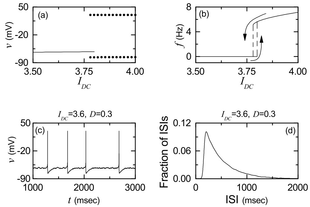 Figure 1
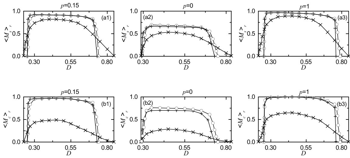 Figure 10
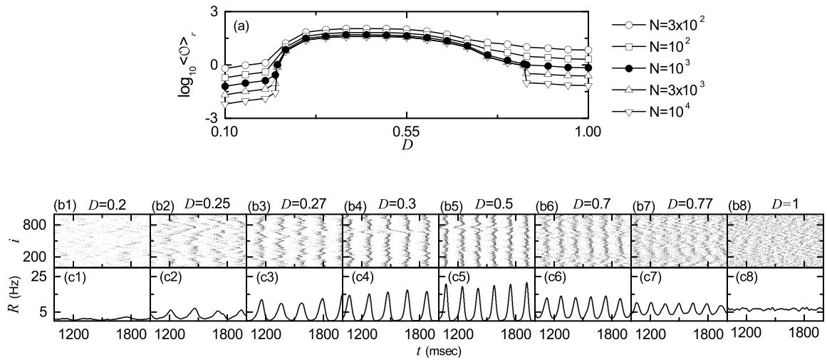 Figure 2
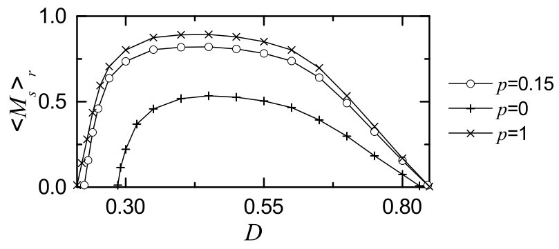 Figure 3
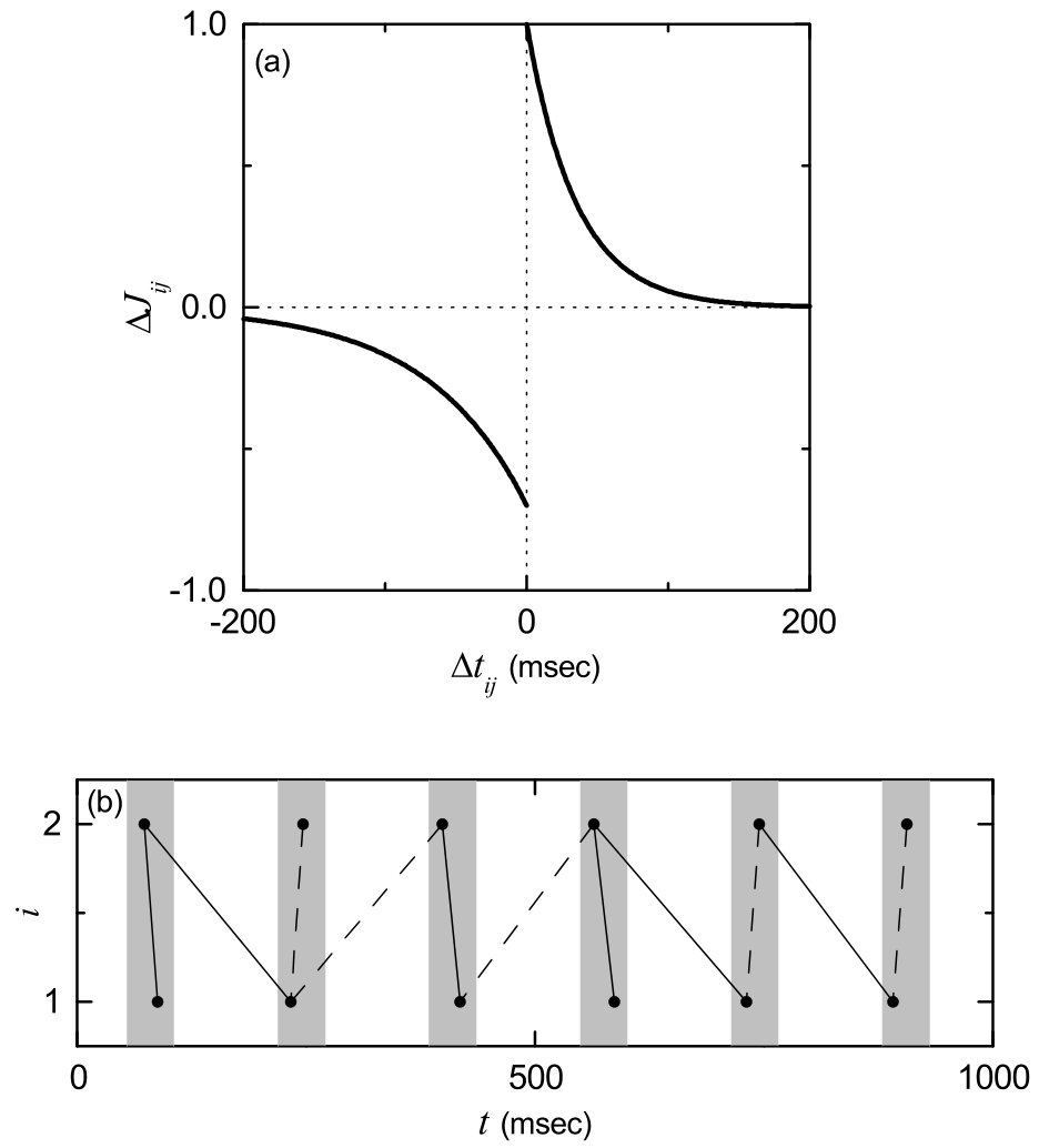 Figure 4
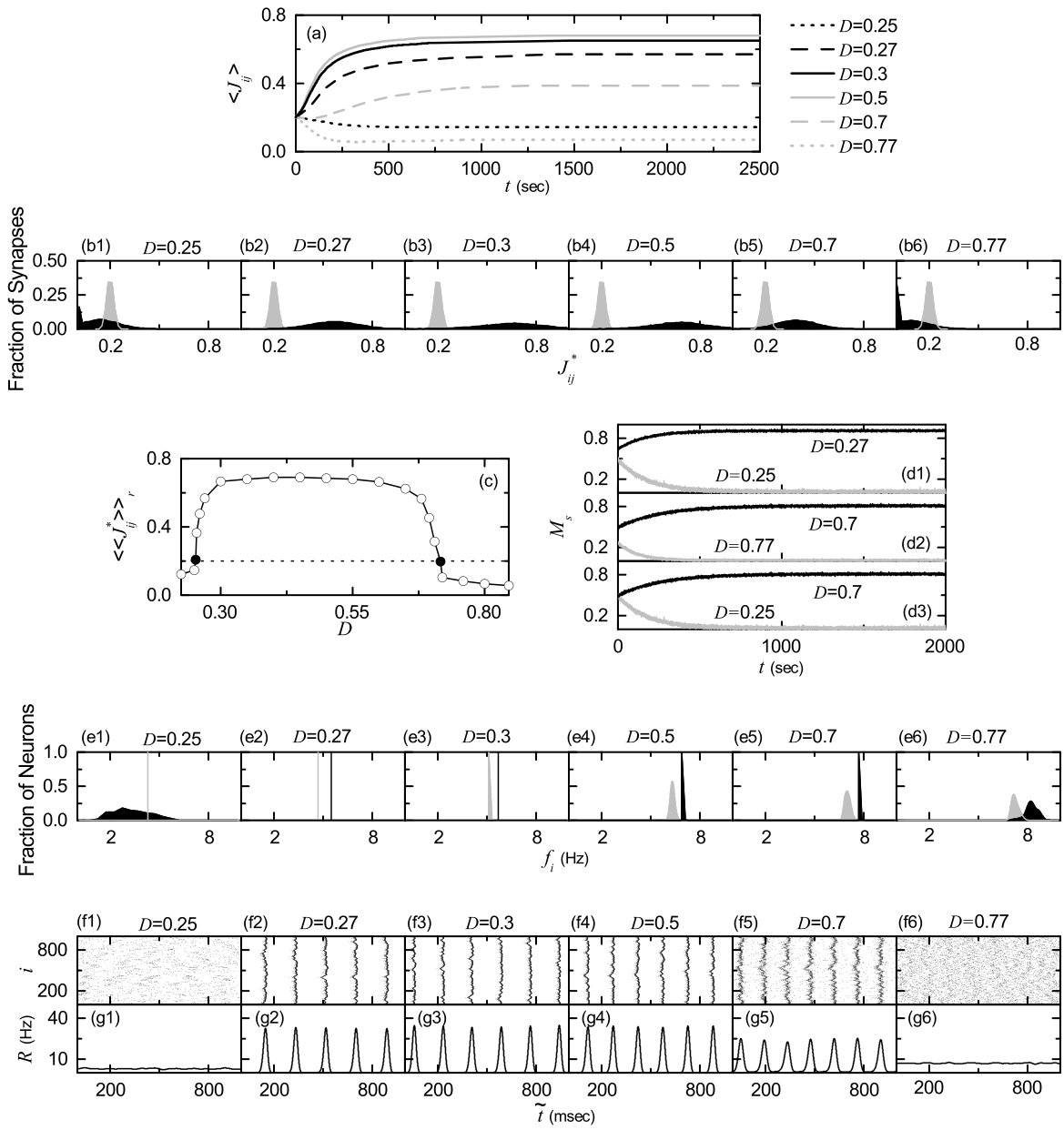 Figure 5
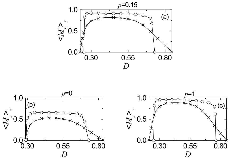 Figure 6
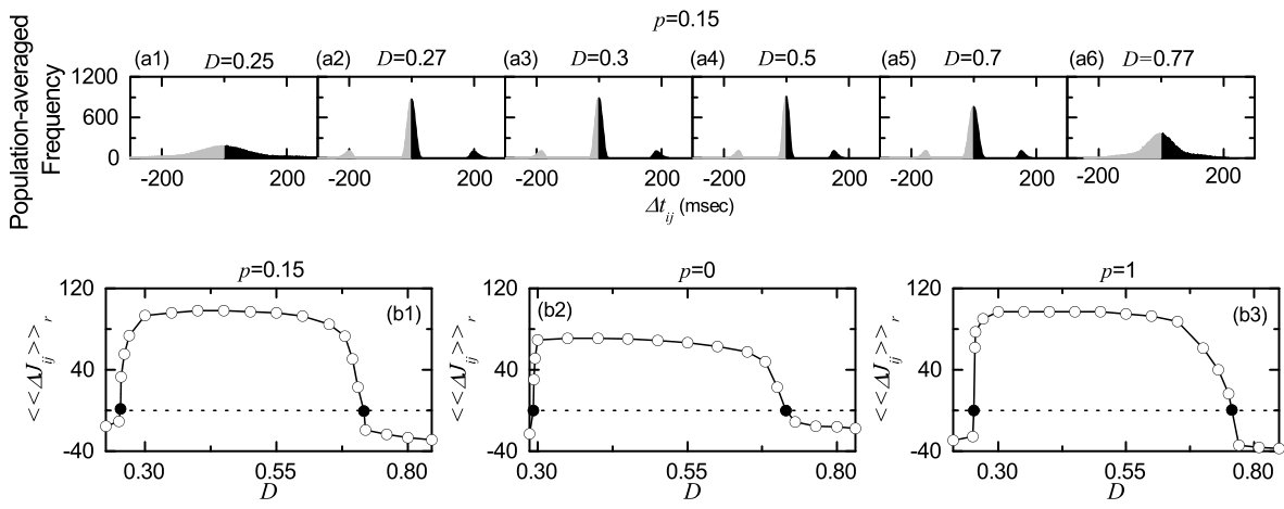 Figure 7
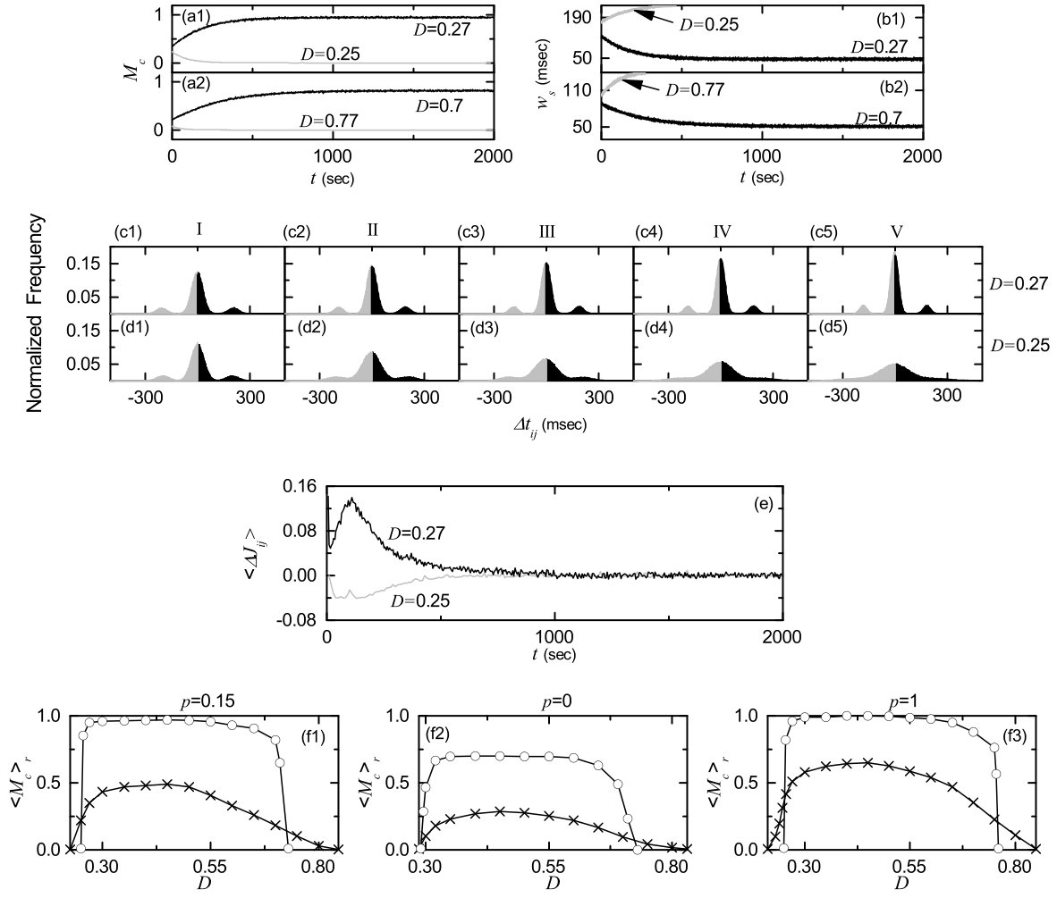 Figure 8
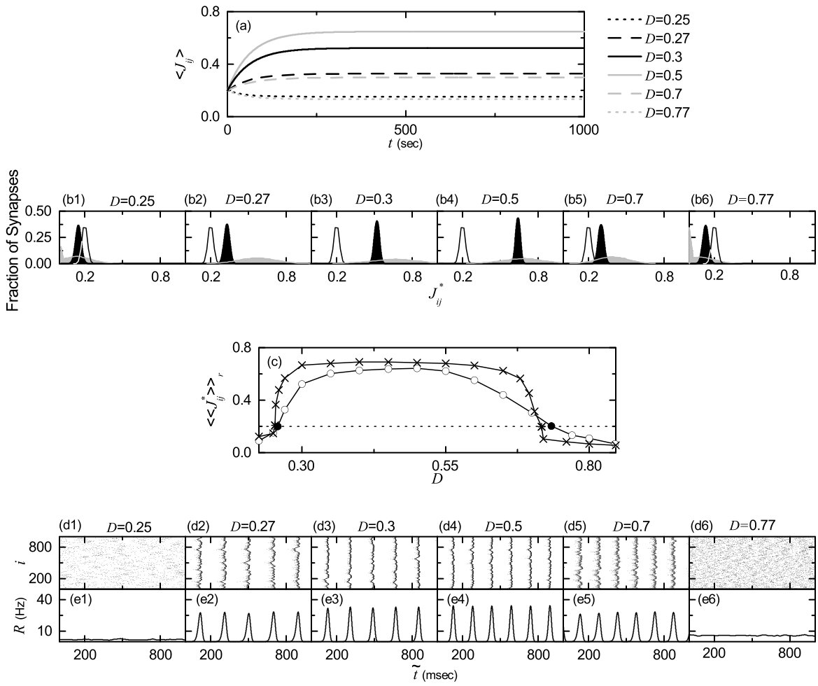 Figure 9
Peer Reviews
No public reviews on file for this paper yet. If you reviewed it on a platform where reviews are public (OpenReview, ICLR, NeurIPS, ICML), you can paste yours below so the community can read it here.
Videos
No videos yet. Explain this paper in a talk, walkthrough, or lecture? Add one.
Taxonomy
TopicsNeural dynamics and brain function · Advanced Memory and Neural Computing · stochastic dynamics and bifurcation
Stochastic Spike Synchronization in A Small-World Neural Network with Spike-Timing-Dependent Plasticity
Sang-Yoon Kim
Woochang Lim
Institute for Computational Neuroscience and Department of Science Education, Daegu National University of Education, Daegu 42411, Korea
Abstract
We consider the Watts-Strogatz small-world network (SWN) consisting of subthreshold neurons which exhibit noise-induced spikings. This neuronal network has adaptive dynamic synaptic strengths governed by the spike-timing-dependent plasticity (STDP). In previous works without STDP, stochastic spike synchronization (SSS) between noise-induced spikings of subthreshold neurons was found to occur in a range of intermediate noise intensities. Here, we investigate the effect of additive STDP on the SSS by varying the noise intensity. Occurrence of a “Matthew” effect in synaptic plasticity is found due to a positive feedback process. As a result, good synchronization gets better via long-term potentiation of synaptic strengths, while bad synchronization gets worse via long-term depression. Emergences of long-term potentiation and long-term depression of synaptic strengths are intensively investigated via microscopic studies based on the pair-correlations between the pre- and the post-synaptic IISRs (instantaneous individual spike rates) as well as the distributions of time delays between the pre- and the post-synaptic spike times. Furthermore, the effects of multiplicative STDP (which depends on states) on the SSS are studied and discussed in comparison with the case of additive STDP (independent of states). These effects of STDP on the SSS in the SWN are also compared with those in the regular lattice and the random graph.
Spike-Timing-Dependent Plasticity, Stochastic Spike Synchronization, Small-World Network, Subthreshold Neurons
pacs:
87.19.lw, 87.19.lm, 87.19.lc
I Introduction
In recent years, much attention has been paid to brain rhythms Buz ; TW . These brain rhythms emerge via population synchronization between individual firings in neural circuits. This kind of neural synchronization is associated with diverse cognitive functions (e.g., multisensory feature integration, selective attention, and memory formation) W_Review ; Gray , and it is also correlated with pathological rhythms related to neural diseases (e.g., tremors in the Parkinson’s disease and epileptic seizures) ND1 ; ND2 . Population synchronization has been intensively investigated in neural circuits composed of spontaneously-firing suprathreshold neurons exhibiting regular discharges like clock oscillators W_Review . In contrast to the case of suprathreshold neurons, the case of subthreshold neurons (which cannot fire spontaneously) has received little attention. The subthreshold neurons can fire only with the help of noise, and exhibit irregular discharges like Geiger counters. Noise-induced firing patterns of subthreshold neurons have been studied in many physiological and pathophysiological aspects Braun1 . For example, sensory receptor neurons were found to use the noise-induced firings for encoding environmental electric or thermal stimuli through a “constructive” interplay of subthreshold oscillations and noise Braun2 . These noise-induced firings of a single subthreshold neuron become most coherent at an optimal noise intensity, which is called coherence resonance Longtin . Moreover, array-enhanced coherence resonance was also found to occur in a population of subthreshold neurons CR1 ; CR2 ; CR3 ; CR4 ; CR5 . In this way, in certain circumstances, noise plays a constructive role in the emergence of dynamical order, although it is usually considered as a nuisance, degrading the performance of dynamical systems.
Here, we are interested in stochastic spike synchronization (SSS) (i.e., population synchronization between complex noise-induced firings of subthreshold neurons) which may be correlated with brain function of encoding sensory stimuli in the noisy environment. Recently, such SSS has been found to occur in an intermediate range of noise intensity via competition between the constructive and the destructive roles of noise Lim1 ; Lim2 ; Lim3 . As the noise intensity passes a lower threshold, a transition to SSS occurs because of a constructive role of noise to stimulate coherence between noise-induced spikings. However, when passing a higher threshold, another transition from SSS to desynchronization takes place due to a destructive role of noise to spoil the SSS. In the previous works on SSS, synaptic coupling strengths were static. However, in real brains synaptic strengths may vary to adapt to the environment (i.e., they can be potentiated LTP1 ; LTP2 ; LTP3 or depressed LTD1 ; LTD2 ; LTD3 ; LTD4 ). These adjustments of synapses are called the synaptic plasticity which provides the basis for learning, memory, and development Abbott1 . Regarding the synaptic plasticity, we consider a Hebbian spike-timing-dependent plasticity (STDP) EtoE0 ; EtoE1 ; EtoE2 ; EtoE3 ; EtoE4 ; EtoE5 ; EtoE6 ; EtoE7 ; EtoE8 ; STDP1 ; STDP2 ; STDP3 ; STDP4 ; STDP5 ; STDP6 ; STDP7 ; STDP8 . For the STDP, the synaptic strengths vary via a Hebbian plasticity rule depending on the relative time difference between the pre- and the post-synaptic spike times. When a pre-synaptic spike precedes a post-synaptic spike, long-term potentiation occurs; otherwise, long-term depression appears. The effects of STDP on population synchronization in networks of (spontaneously-firing) suprathreshold neurons were studied in various aspects Brazil1 ; Brazil2 ; Tass1 ; Tass2 .
In this paper, we consider an excitatory Watts-Strogatz small-world network (SWN) of subthreshold neurons SWN1 ; SWN2 ; SWN3 , and investigate the effect of additive STDP (independent of states) on the SSS by varying the noise intensity . A Matthew effect in synaptic plasticity is found to occur due to a positive feedback process. Good synchronization gets better via long-term potentiation of synaptic strengths, while bad synchronization gets worse via long-term depression. As a result, a step-like rapid transition to SSS occurs by changing , in contrast to the relatively smooth transition in the absence of STDP. Emergences of long-term potentiation and long-term depression of synaptic strengths are intensively studied through microscopic investigations based on both the distributions of time delays between the pre- and the post-synaptic spike times and the pair-correlations between the pre- and the post-synaptic IISRs (instantaneous individual spike rates). Moreover, the effects of multiplicative STDP (which depends on states) on the SSS are also studied Tass1 ; Multi . For the multiplicative case, a change in synaptic strengths scales linearly with the distance to the higher and the lower bounds of synaptic strengths, and hence the bounds for the synaptic strength become “soft,” in contrast to the hard bounds for the additive case. The effects of STDP for the multiplicative case with soft bounds are discussed in comparison with the additive case with hard bounds. Moreover, the effects of additive and multiplicative STDP on the SSS in the SWN are also compared with those in the regular lattice and the random graph.
This paper is organized as follows. In Sec. II, we describe an excitatory Watts-Strogatz SWN of subthreshold Izhikevich regular spiking neurons Izhi1 ; Izhi2 , and the governing equations for the population dynamics are given. Then, in Sec. III we investigate the effects of STDP on the SSS for both the additive and the multiplicative cases by varying . Finally, in Sec. IV a summary is given.
II Excitatory Small-World Network of Subthreshold Neurons with Synaptic Plasticity
We consider an excitatory directed Watts-Strogatz SWN, composed of subthreshold regular spiking neurons equidistantly placed on a one-dimensional ring of radius . The Watts-Strogatz SWN interpolates between a regular lattice with high clustering (corresponding to the case of ) and a random graph with short average path length (corresponding to the case of ) via random uniform rewiring with the probability SWN1 ; SWN2 ; SWN3 . For we start with a directed regular ring lattice with nodes where each node is coupled to its first neighbors ( on either side) via outward synapses, and rewire each outward connection uniformly at random over the whole ring with the probability (without self-connections and duplicate connections). This Watts-Strogatz SWN model may be regarded as a cluster-friendly extension of the random network by reconciling the six degrees of separation (small-worldness) SDS1 ; SDS2 with the circle of friends (clustering). Many recent works on various subjects of neurodynamics have been done in SWNs with predominantly local connections and rare long-distance connections SW1 ; SW2 ; SW3 ; SW4 ; SW5 ; SW6 ; SW7 ; SW8 ; SW9 ; SW10 ; SW11 ; SW12 ; SW13 . As elements in our SWN, we choose the Izhikevich regular spiking neuron model which is not only biologically plausible, but also computationally efficient Izhi1 ; Izhi2 .
The following equations (1)-(6) govern the population dynamics in the SWN:
[TABLE]
with the auxiliary after-spike resetting:
[TABLE]
where
[TABLE]
Here, and are the state variables of the th neuron at a time which represent the membrane potential and the recovery current, respectively. These membrane potential and the recovery variable, and , are reset according to Eq. (3) when reaches its cutoff value . The parameter values used in our computations are listed in Table 1. More details on the Izhikevich regular spiking neuron model, the external stimulus to each Izhikevich regular spiking neuron, the synaptic currents and plasticity, and the numerical method for integration of the governing equations are given in the following subsections.
II.1 Izhikevich Regular Spiking Neuron Model
We first note that the function in Eq. (4) for the dynamics of the Izhikevich neuron was obtained by fitting the spike initiation dynamics of a cortical neuron so that the membrane potential has mV scale and the time has msec scale Izhi1 ; Izhi2 . Then, the Izhikevich model may match neuronal dynamics by tuning the parameters instead of matching neuronal electrophysiology, unlike the Hodgkin-Huxley-type conductance-based models Izhi1 ; Izhi2 . The parameters , , , and are related to the time scale of the recovery variable , the sensitivity of to the subthreshold fluctuations of , and the after-spike reset values of and , respectively. Depending on the values of these parameters, the Izhikevich neuron model may exhibit 20 of the most prominent neuro-computational features of cortical neurons Izhi1 ; Izhi2 . Here, we use the parameter values for the regular spiking neurons, which are listed in the 1st item of Table 1.
II.2 External Stimulus to Each Izhikevich Regular Spiking Neuron
Each Izhikevich regular spiking neuron is stimulated by both a common DC current and an independent Gaussian white noise [see the 3rd and the 4th terms in Eq. (1)]. The Gaussian white noise satisfies and , where denotes an ensemble average. Here, the intensity of the Gaussian noise is controlled by the parameter . For , the Izhikevich regular spiking neurons exhibit the type-II excitability. A type-II neuron exhibits a jump from a resting state to a spiking state through a subcritical Hopf bifurcation when passing a threshold by absorbing an unstable limit cycle born via fold limit cycle bifurcation and hence, the firing frequency begins from a non-zero value Ex1 ; Ex2 . Throughout the paper, we consider a subthreshold case (where only noise-induced firings occur) such that the value of is chosen via uniform random sampling in the range of [3.55, 3.65], as shown in the 2nd item of Table 1.
II.3 Synaptic Currents and Plasticity
The 5th term in Eq. (1) denotes the synaptic couplings of Izhikevich regular spiking neurons. of Eq. (5) represents the synaptic current injected into the th neuron, and is the synaptic reversal potential. The synaptic connectivity is given by the connection weight matrix (=) where if the neuron is presynaptic to the neuron ; otherwise, . Here, the synaptic connection is modeled in terms of the Watts-Strogatz SWN. The in-degree of the th neuron, (i.e., the number of synaptic inputs to the neuron ) is given by . For this case, the average number of synaptic inputs per neuron is given by . Throughout the paper, (see the 4th item of Table 1).
The fraction of open synaptic ion channels at time is denoted by . The time course of of the th neuron is given by a sum of delayed double-exponential functions [see Eq. (6)], where is the synaptic delay, and and are the th spiking time and the total number of spikes of the th neuron (which occur until time ), respectively. Here, [which corresponds to contribution of a pre-synaptic spike occurring at time [math] to in the absence of synaptic delay] is controlled by the two synaptic time constants: synaptic rise time and decay time , and is the Heaviside step function: for and 0 for . For the excitatory AMPA synapse, the values of , , , and are listed in the 3rd item of Table 1 AMPA .
The coupling strength of the synapse from the th pre-synaptic neuron to the th post-synaptic neuron is . Here, we consider a Hebbian STDP for the synaptic strengths . Initial synaptic strengths are normally distributed with the mean and the standard deviation . With increasing time , the synaptic strength for each synapse is updated with an additive nearest-spike pair-based STDP rule SS :
[TABLE]
where is the update rate and is the synaptic modification depending on the relative time difference between the nearest spike times of the post-synaptic neuron and the pre-synaptic neuron . To avoid unbounded growth and negative conductances (i.e. negative coupling strength), we set a range with the upper and the lower bounds: . Specifically, the upper bound of is set to to avoid occurrence of noise-induced burtsings for a strong excitatory coupling NB , and the lower boundary is set to (i.e., slightly greater than 0) to avoid elimination of synaptic connections. We use an asymmetric time window for the synaptic modification STDP1 :
[TABLE]
where , , msec, msec (these values are also given in the 5th item of Table 1), and .
II.4 Numerical Method for Integration
Numerical integration of stochastic differential Eqs. (1)-(6) with a Hebbian STDP rule of Eqs. (7) and (8) is done by employing the Heun method SDE with the time step msec. For each realization of the stochastic process, we choose random initial points for the th regular spiking neuron with uniform probability in the range of and .
III Effects of the STDP on the Stochastic Spike Synchronization
We consider the Watts-Strogatz SWN with high clustering and short path length when the rewiring probability is 0.15. This SWN is composed of excitatory subthreshold Izhikevich regular spiking neurons (exhibiting noise-induced spikings). Throughout the paper, except for the case of the order parameter in Fig. 2(a). As shown in Fig. 1(a), the Izhikevich regular spiking neuron exhibits a jump from a resting state (denoted by a solid line) to a spiking state (represented by solid circles) via subcritical Hopf bifurcation at a higher threshold by absorbing an unstable limit cycle born through a fold limit cycle bifurcation for a lower threshold . Hence, the Izhikevich regular spiking neuron exhibits type-II excitability because it begins to fire with a non-zero frequency Ex1 ; Ex2 . Figure 1(b) shows a plot of the mean firing rate (MFR) versus the external DC current for a single Izhikevich regular spiking neuron in the absence of noise (). As is increased from , the MFR increases monotonically. As an example, we consider a subthreshold case of in the presence of noise with for which a time series of the membrane potential with the MFR Hz is shown in Fig. 1(c). Figure 1(d) also shows a histogram for distribution of interspike intervals (ISIs) for and . The average ISI is 506.3 msec; the reciprocal of corresponds to the MFR. This distribution is also broad because of a large standard deviation (=350.2 msec) from the average value.
III.1 SSS in The Absence of STDP
First, we are concerned about the SSS in the absence of STDP. The coupling strengths are static, and their values are chosen from the Gaussian distribution where the mean is 0.2 and the standard deviation is 0.02. Population synchronization may be well visualized in the raster plot of neural spikes which is a collection of spike trains of individual neurons. Such raster plots of spikes are fundamental data in experimental neuroscience. As a collective quantity showing population behaviors, we use an instantaneous population spike rate (IPSR) which may be obtained from the raster plots of spikes W_Review ; RM . For the synchronous case, “stripes” (composed of spikes and indicating population synchronization) are found to be formed in the raster plot, while in the unsynchronized case spikes are completely scattered. Hence, for a synchronous case, an oscillating IPSR appears, while for an unsynchronized case is nearly stationary. To obtain a smooth IPSR, we employ the kernel density estimation (kernel smoother) Kernel . Each spike in the raster plot is convoluted (or blurred) with a kernel function to obtain a smooth estimate of IPSR :
[TABLE]
where is the th spiking time of the th neuron, is the total number of spikes for the th neuron, and we use a Gaussian kernel function of band width :
[TABLE]
Throughout the paper, the band width of is 10 msec. Recently, we introduced a realistic thermodynamic order parameter, based on , for describing transition from desynchronization to synchronization RM . The mean square deviation of ,
[TABLE]
plays the role of an order parameter ; the overbar represents the time average. This order parameter may be regarded as a thermodynamic measure because it concerns just the macroscopic IPSR kernel estimate without any consideration between and microscopic individual spikes. In the thermodynamic limit of , the order parameter approaches a non-zero (zero) limit value for the synchronized (unsynchronized) state. Figure 2(a)shows plots of versus in the SWN with for . In each realization, we discard the first time steps of a stochastic trajectory as transients for msec, and then we numerically compute by following the stochastic trajectory for msec. Throughout the paper, denotes an average over 20 realizations. With increasing up to , these numerical calculations for are done for various values of . For ), unsynchronized states exist because the order parameter tends to decrease to zero as is increased. As passes the lower threshold , tends to converge toward non-zero limit values, and hence a transition to SSS occurs thanks to a constructive role of noise to stimulate coherence between noise-induced spikings of subthreshold neurons. However, for large , with increasing the order parameter tends to approach zero, and hence SSS disappears (i.e., a transition to desynchronization occurs when passes the higher threshold ) due to a destructive role of noise to spoil the SSS. In this way, SSS appears in an intermediate range of via competition between the constructive and the destructive roles of noise. Figures 2(b1)-2(b8) show raster plots of spikes for various values of , and their corresponding IPSR kernel estimates are also shown in Figs. 2(c1)-2(c8). For (less than ), spikes are scattered without forming any stripes in the raster plot, and hence the IPSR kernel estimate is nearly stationary. On the other hand, when passing , synchronized states appear. For the raster plot of spikes shows a zigzag pattern intermingled with inclined partial stripes of spikes due to local clustering, and the IPSR kernel estimate exhibits an oscillatory behavior. With increasing the degree of SSS is increased because clearer stripes with reduced zigzagness appear (e.g., see the cases of 0.3, and 0.5). As a result, the amplitude of increases with . However, with further increase in , stripes are smeared, as shown in the cases of and 0.77, and hence the amplitude of decreases. Eventually, when passing desynchronization occurs due to overlap of smeared stripes (e.g., see the case of ). We also note that the population frequency of the IPSR kernel estimate increases with in the range of SSS (i.e., the interval between stripes in the raster plots of spikes decreases with ).
We characterize the SSS by employing the statistical-mechanical spiking measure RM . For the case of SSS, stripes appear regularly in the raster plot of spikes. The spiking measure of the th stripe is defined by the product of the occupation degree of spikes (representing the density of the th stripe) and the pacing degree of spikes (denoting the smearing of the th stripe):
[TABLE]
The occupation degree of spikes in the stripe is given by the fraction of spiking neurons:
[TABLE]
where is the number of spiking neurons in the th stripe. For the full occupation , while for the partial occupation . In our case of SSS, , independently of . For this case of full synchronization, . The pacing degree of spikes in the th stripe can be determined in a statistical-mechanical way by taking into account their contributions to the macroscopic IPSR kernel estimate . Central maxima of between neighboring left and right minima of coincide with centers of stripes in the raster plot. A global cycle starts from a left minimum of , passes a maximum, and ends at a right minimum. An instantaneous global phase of was introduced via linear interpolation in the region forming a global cycle (for details, refer to Eqs. (16) and (17) in RM ). Then, the contribution of the th microscopic spike in the th stripe occurring at the time to is given by , where is the global phase at the th spiking time [i.e., ]. A microscopic spike makes the most constructive (in-phase) contribution to when the corresponding global phase is (), while it makes the most destructive (anti-phase) contribution to when is . By averaging the contributions of all microscopic spikes in the th stripe to , we obtain the pacing degree of spikes in the th stripe:
[TABLE]
where is the total number of microscopic spikes in the th stripe. By averaging over a sufficiently large number of stripes, we obtain the realistic statistical-mechanical spiking measure , based on the IPSR kernel estimate :
[TABLE]
We follow stripes in each realization and get via average over 20 realizations. Figure 3 shows a plot of (denoted by open circles) versus in the SWN with . When passing a rapid increase in occurs, then a flat “plateau” of appears, and finally decreases in a relatively slow way. Thus, a bell-shaped curve (composed of open circles) is formed. For comparison, we also consider the cases of (regular lattice) and (random graph); the cases of and 1 are represented by pluses and crosses, respectively. The topological properties of the small-world connectivity has been well characterized in terms of the clustering coefficient and the average path length SWN1 . The clustering coefficient , representing the cliquishness of a typical neighborhood in the network, characterizes the local efficiency of information transfer, while the average path length , denoting the typical separation between two vertices in the network, characterizes the global efficiency of information transfer. Particularly, short path length may be efficient for global communication between distant neurons (i.e. neural synchronization). The regular lattice for is highly clustered but large world where the average path length grows linearly with SWN1 ; and for . On the other hand, the random graph for is poorly clustered but small world where the average path length grows logarithmically with SWN1 ; and for . As soon as increases from zero, the average path length decreases dramatically, which leads to occurrence of a small-world phenomenon which is popularized by the phrase of the “six degrees of separation” SDS1 ; SDS2 . However, during such dramatic drop in , the clustering coefficient decreases only a little. Consequently, for small (=0.15) an SWN with short path length and high clustering emerges. for is much smaller than that for (regular lattice), and it is just a little larger than that for (random graph). Hence, the values of for are much larger than those for , and they are somewhat close to those for . However, unlike the case of , zigzag patterns of partially inclined stripes appear in the raster plot of spikes for due to high local clustering, as shown in Figs. 2(b2)-2(b7).
III.2 Effects of The Additive STDP on The SSS
From now on, we study the effect of additive STDP on the SSS. The initial values of synaptic strengths are chosen from the Gaussian distribution where the mean is 0.2 and the standard deviation is 0.02. Then, for each synapse is updated according to the additive nearest-spike pair-based STDP rule of Eq. (7) SS . Figure 4(a) shows the time window for the synaptic modification of Eq. (8) (i.e., plot of versus ). varies depending on the relative time difference between the nearest spike times of the post-synaptic neuron and the pre-synaptic neuron . When a post-synaptic spike follows a pre-synaptic spike (i.e., is positive), long-term potentiation of synaptic strength appears; otherwise (i.e., is negative), long-term depression occurs. A schematic diagram for the nearest-spike pair-based STDP rule is given in Fig. 4(b), where and 2 correspond to the post- and the pre-synaptic neurons. Here, gray boxes represent stripes in the raster plot, and spikes in the stripes are denoted by solid circles. When the post-synaptic neuron () fires a spike, long-term potentiation (denoted by solid lines) occurs via STDP between the post-synaptic spike and the previous nearest pre-synaptic spike. In contrast, when the pre-synaptic neuron () fires a spike, long-term depression (represented by dashed lines) occurs through STDP between the pre-synaptic spike and the previous nearest post-synaptic spike. We note that such long-term potentiation and long-term depression may occur between the pre- and the post-synaptic spikes in the same stripe or in the different nearest-neighboring stripes; solid/dashed lines connect pre- and post-synaptic spikes in the same stripe or in the different nearest-neighboring stripes.
Figure 5(a) shows time-evolutions of population-averaged synaptic strengths for various values of in the SWN with ; represents an average over all synapses. For each case of 0.3, 0.5 and 0.7, increases monotonically above its initial value (=0.2), and it approaches a saturated limit value nearly at sec. Consequently, long-term potentiation occurs for these values of . On the other hand, for and 0.77, decreases monotonically below , and approaches a saturated limit value . As a result, long-term depression occurs for the cases of and 0.77. Histograms for fraction of synapses versus (saturated limit values of at sec) are shown in black color for various values of in Figs. 5(b1)-5(b6); the bin size for each histogram is 0.02. For comparison, initial distributions of synaptic strengths (i.e., Gaussian distributions whose mean and standard deviation are 0.2 and 0.02, respectively) are also shown in gray color. For the cases of long-term potentiation ( 0.3, 0.5 and 0.7), their black histograms lie on the right side of the initial gray histograms, and hence their population-averaged values become larger than the initial value (=0.2). In contrast, the black histograms for the cases of long-term depression ( and 0.77) are shifted to the left side of the initial gray histograms, and hence their population-averaged values become smaller than . For both cases of long-term potentiation and long-term depression, their black histograms are much wider than the initial gray histograms [i.e., the standard deviations are very larger than the initial one (=0.02)]. Figure 5(c) shows a plot of population-averaged limit values of synaptic strengths versus . Here, the horizontal dotted line represents the initial average value of coupling strengths (= 0.2), and the lower and the higher threshold values and for long-term potentiation and long-term depression (where ) are denoted by solid circles. Hence, long-term potentiation occurs in the range of (, ); otherwise, long-term depression appears. We also note that the range of (, ) is strictly contained in the range of (, ) ( and ) where SSS appears in the absence of STDP [i.e., (, ) is a proper subset of (, )]. Hence, in most range of the SSS long-term potentiation occurs, while long-term depression takes place only near both ends. Similar to the case in Fig. 5(c), a bell-shaped curve (showing a plot of average synaptic strengths versus noise intensity) was also observed for the case where many nearly coincident pre-synaptic inputs are given to a post-synaptic neuron Aihara .
We now consider the effects of long-term potentiation and long-term depression on the SSS for . Time-evolutions of the statistical-mechanical spiking measures [of Eq. (15)] for the population states are shown in Figs. 5(d1)-5(d3); black (gray) curves represent the cases of long-term potentiation (long-term depression). For the case of close small values of in Fig. 5(d1), the initial value of for is a little larger than that for . However, with increasing time , for increases thanks to long-term potentiation, and it approaches its limit value. On the other hand, for decreases due to long-term depression, and it seems to approach zero (i.e., desynchronization occurs). A similar one takes place for the case of close large values of in Fig. 5(d2). The initial value of for is a little larger than that for . But, as the time increases, for increases thanks to long-term potentiation, while for decreases due to long-term depression. Furthermore, we note that for (0.25) increases (decreases) due to long-term potentiation (long-term depression), although their initial values of are nearly the same [see Fig. 5(d3)]. This seems to occur because MFRs of individual neurons for are higher than those for . For the case of higher MFR, the distribution of may be narrower, which seems to lead to long-term potentiation STDP7 ; Tass2 . Figures 5(e1)-5(e6) show the histograms for MFRs of individual neurons in black color for various values of ; the MFR for each neuron is obtained through averaging of msec after the saturation time ( sec) and the bin size for each histogram is 0.2 Hz. For comparison, initial distributions for are shown in gray color. In the case of long-term potentiation ( 0.3, 0.5, and 0.7), both the population frequency of the IPSR kernel estimate and the degree of SSS increase, in comparison with those in the absence of STDP [compare Figs. 5(f2)-5(f5) and Figs. 5(g2)-5(g5) with Figs. 2(b3)-2(b6) and Figs. 2(c3)-2(c6)]. As a result, the population-averaged MFRs become higher (i.e., black histograms lie on the right side of the initial gray histograms), and their standard deviations from are generally smaller (i.e., widths of the black histograms are generally narrower) except for the case of small (=0.27) where the standard deviations are the same in both the presence and the absence of STDP. For the case of long-term depression ( and 0.77), the population states become desynchronized. Without any coherent synaptic inputs, individual neurons fire randomly mainly due to noise. Hence, for large (=0.77) the population-averaged MFR increases, while for small (=0.25) becomes smaller. For both cases, the standard deviations of their distributions become larger because of the noise effect. Neural synchronization may be well visualized in the raster plot of spikes, and the corresponding IPSR kernel estimate shows the population behaviors well. Figures 5(f1)-5(f6) and Figures 5(g1)-5(g6) show raster plots of spikes and the corresponding IPSR kernel estimates for various values of , respectively. When compared with Figs. 2(b2)-2(b7) and Figs. 2(c2)-2(c7) in the absence of STDP, the degrees of SSS for the case of long-term potentiation ( 0.3, 0.5 and 0.7) are increased so much, while in the case of long-term depression ( and 0.77) the population states become desynchronized.
We characterize the SSS in terms of the statistical-mechanical spiking measure , which is also compared with the case without STDP. Figure 6(a) shows the plot of (represented by open circles) versus in the SWN with ; for comparison, in the absence of STDP are shown in crosses. A Matthew effect in synaptic plasticity occurs via a positive feedback process. Good synchronization gets better through long-term potentiation, while bad synchronization gets worse through long-term depression. Consequently, a rapid step-like transition to SSS takes place, which is in contrast to the relatively smooth transition in the absence of STDP. For comparison with the case of SWN with , we also consider the cases of (regular lattice) and (random graph). The regular lattice is highly clustered but large world, while the random graph is poorly clustered but small world. As a cluster-friendly extension of the random graph, the SWN has both high clustering and short path length. Figures 6(b) and 6(c) show plots of (denoted by open circles) for and 1, respectively; in the absence of STDP are also shown in crosses. As in the SWN, Matthew effects in synaptic plasticity occur in both cases of and 1, and hence rapid transitions to SSS occur. The degree of SSS (given by ) for the case of SWN with is much larger than that for the case of because the average path length for the SWN with is much shorter than that for . is dramatically decreased with increasing , and hence for is close to that for . As a result, for is close to that for . Moreover, as is increased, transitions to SSS become more rapid due to the increased Matthew effect.
From now on, we make an intensive investigation on emergences of long-term potentiation and long-term depression of synaptic strengths via microscopic studies based on the distributions of time delays between the pre- and the post-synaptic spike times. Figures 7(a1)-7(a6) show population-averaged histograms for the distributions of time delays during the time interval from to the saturation time ( sec) for various values of in the SWN with : for each synaptic pair, its histogram for the distribution of is obtained, and then we get the population-averaged histogram via averaging over all synaptic pairs. Here, black and gray regions represent long-term potentiation and long-term depression, respectively. In the case of long-term potentiation ( 0.3, 0.5, and 0.7), 3 peaks appear: one main central peak and two left and right minor peaks. When the pre- and the post-synaptic spike times appear in the same spiking stripe in the raster plot of spikes, its time delay lies in the main peak; long-term potentiation and long-term depression may occur depending on the sign of . On the other hand, time delays lie in the minor peaks when the pre- and the post-synaptic spike times appear in the different nearest-neighboring spiking stripes. If the pre-synaptic stripe precedes the post-synaptic stripe (causality), then its time delay lies in the right minor peak (long-term potentiation); otherwise, it lies in the left minor peak (long-term depression). For the case of long-term depression ( and 0.77), the population states become desynchronized due to overlap of spiking stripes in the raster plot of spikes. Consequently, the main peak in the histogram becomes merged with the left and the right minor peaks, and then only one broadened main peak appears, in contrast to the case of long-term potentiation. The population-averaged synaptic modification [during the time interval from to the saturation time ( sec)] may be directly obtained from the above histogram :
[TABLE]
Figure 7(b1) shows a plot of [obtained from ] versus for ; solid circles represent the lower and the higher thresholds and for long-term potentiation and long-term depression (where ) which are the same as those in Fig. 5(c). Then, population-averaged limit values of synaptic strengths are given by , which agree well with the directly-obtained values in Fig. 5(c). Similarly, for (regular lattice) and 1 (randon graph), we also obtain population-averaged synaptic modification from the population-averaged histograms for the distributions of time delays during the time interval from to the saturation time ( sec), which are shown in Figs. 7(b2) and 7(b3), respectively. As is increased from 0, the range of long-term potentiation [i.e., (, )] becomes wider and most synaptic modifications for the long-term potentiation are also increased.
Finally, we study the effect of STDP on the microscopic pair-correlation between the pre- and the post-synaptic IISRs (instantaneous individual spike rates) for the synaptic pair. For obtaining dynamical pair-correlations, each spike train of the th neuron is convoluted with a Gaussian kernel function of band width to get a smooth estimate of IISR :
[TABLE]
where is the th spiking time of the th neuron, is the total number of spikes for the th neuron, and is given in Eq. (10). Then, the normalized temporal cross-correlation function between the IISR kernel estimates and of the synaptic pair is given by:
[TABLE]
where and the overline denotes the time average. Then, the microscopic correlation measure representing the average “in-phase” degree between the pre- and the post-synaptic pairs, is given by the average value of at the zero-time lag for all synaptic pairs:
[TABLE]
where is the total number of synapses. Time-evolutions of the microscopic correlation measures for the population states are shown in Figs. 8(a1)-8(a2) for the case of SWN with . Data for calculation of are obtained via averages during successive 5 global cycles of the IPSR kernel estimate for the case of long-term potentiation, while the data for the case of long-term depression are obtained through averages during successive 5 global cycles of for sec and during successive 100 global cycles for sec. For the case of close small values of in Fig. 8(a1), the initial value of for is a little larger than that for . However, with increasing time , for increases, and it approaches a limit value. On the other hand, for decreases with time , and it seems to approach zero. A similar one occurs in the case of close large values of in Fig. 8(a2). The initial value of for is a little larger than that for . But, as the time increases, for increases, while for decreases. Enhancement (suppression) in results in increase (decrease) in the average in-phase degree between the pre- and the post-synaptic pairs. Then, widths of spiking stripes in the raster plot of spikes decrease (increase) due to enhancement (suppression) of . Figures 8(b1)-8(b2) show time-evolutions of the width of the spiking stripes for ; is obtained through averaging the widths of spiking stripes during successive 5 global cycles of . For and 0.7, decreases thanks to enhancement in , which leads to narrowed distribution of time delays between the pre- and the post-synaptic spike times. Consequently, long-term potentiation may occur. In contrast, for and 0.77, increases due to suppression in (calculations of for 0.25 and 0.77 are made until 464 sec and 273 sec, respectively, when spiking stripes begin to overlap), which results in widened distribution of time delays . As a result, long-term depression may takes place.
Time-evolutions of normalized histograms for the distributions of time delays are shown for in Figs. 8(c1)-8(c5) and for in Figs. 8(d1)-8(d5) when ; the bin size in each histogram is 2 msec. Here, we consider 5 stages [represented by I (starting from sec), II (starting from sec), III (starting from sec), IV (starting from sec), and V (starting from sec)]; for more details, refer to the caption of Fig. 8. At each stage, we get distribution for for all synaptic pairs during the 5 global cycles (about 1 sec) of the IPSR kernel estimate and obtain normalized histogram by dividing the distribution with the total number of synapses (=20000). For (long-term potentiation), 3 peaks appear in each histogram; main central peak and two left and right minor peaks. With increasing the time (i.e., with increase in the level of stage), peaks become narrowed, and then they become sharper. Two minor peaks also approach the main peak a little because the population frequency of increases with the stage. Furthermore, as the stage is increased, the main peak becomes more and more symmetric, and hence the effect of long-term potentiation in the black part tends to cancel out nearly the effect of long-term depression in the gray part at the stage V. For (long-term depression), with increasing the level of the stage, peaks become wider and the merging-tendency between the peaks is intensified. At the stages IV and V, only one broad central peak seems to appear. For the stage V, the effect of long-term potentiation in the black part tends to cancel out nearly the effect of long-term depression in the gray part because the broad peak is nearly symmetric. From these normalized histograms [obtained via averages during successive 5 global cycles of ], we also get the population-averaged synaptic modification []. Figure 8(e) shows time-evolutions of for (black curve) and (gray curve) when . for is positive, while it is negative for . For both cases, they converge toward nearly zero at the stage V sec) because the normalized histograms become nearly symmetric. Then, the time evolution of population-averaged synaptic strength is given by where represents the average for the th 5 global cycles of and (initial average synaptic strength)= 0.2. Time-evolutions of (obtained in this way) for and 0.25 agree well with those in Fig. 5(a). As a result, long-term potentiation (long-term depression) occurs for (0.25).
Figure 8(f1) shows plots of versus in the presence (open circles) and the absence (crosses) of STDP for the case of SWN with ; for comparison, the cases of (regular lattice) and (random graph) are also shown in Figs. 8(f2) and 8(f3), respectively. The number of data used for the calculation of each temporal cross-correlation function [the values of at the zero time lag are used for calculation of ] is (=65536) after the saturation time ( sec) in each realization. Like the case of in Fig. 6, a Matthew effect also occurs in : good pair-correlation gets better, while bad pair-correlation gets worse. Hence, a step-like transition occurs, in contrast to the case without STDP. As is increased from 0, such transitions become more rapid due to the increased Matthew effect. Since the average path length for is much smaller than that for and close to that for , the values of on the top plateau for are much larger than those for , and they are so close to those for .
III.3 Effects of The Multiplicative STDP on The SSS
In this subsection, we study the effect of multiplicative STDP (which depends on states) on the SSS in comparison with the (above) additive case. The coupling strength for each synapse is updated with a multiplicative nearest-spike pair-based STDP rule Tass1 ; Multi :
[TABLE]
Here, is the update rate, is the synaptic modification depending on the relative time difference between the nearest spike times of the post-synaptic neuron and the pre-synaptic neuron [time window for is given in Eq. (8)], and for the long-term potentiation (long-term depression) [ and is the higher (lower) bound of (i.e., ]. For this multiplicative case, the bounds for the synaptic strength become soft, because a change in synaptic strengths scales linearly with the distance to the higher and the lower bounds, in contrast to the hard bounds for the case of additive STDP (without dependence on states).
Figure 9(a) shows time-evolutions of population-averaged synaptic strengths for various values of in the SWN with . For 0.3, 0.5 and 0.7, increases above its initial value (= 0.2), and it approaches a saturated limit value nearly at sec. As a result, long-term potentiation occurs for these values of . On the other hand, for and 0.77 decreases below , and approaches a saturated limit value . Consequently, long-term depression occurs for these values of . When compared with the additive case in Fig. 5(a), the saturation time is shorter and deviations of the saturated limit values from are smaller due to the soft bounds. Histograms for fraction of synapses versus (saturated limit values of at sec) for are shown in black regions for various values of in Figs. 9(b1)-9(b6); the bin size for each histogram is 0.02. For comparison, distributions of for the case of the additive STDP and initial Gaussian distributions (mean = 0.2 and standard deviation = 0.02) of are also shown in gray regions and in black curves, respectively. As in the case of additive STDP, long-term potentiation occurs for 0.3, 0.5, and 0.7, because their black histograms lie on the right side of the initial black-curve histograms. However, these black histograms lie on the left side of the gray histograms for the case of additive STDP, and they are much narrower than those for the additive case. Consequently, their population-averaged values and standard deviations are smaller than those for the additive case, because their variations in are restricted due to soft bounds in comparison with hard bounds for the the additive case. Particularly, the standard deviations for the multiplicative case are even smaller than the initial ones (= 0.02). On the other hand, for and 0.77 long-term depression occurs because the black histograms are shifted to the left side of the initial black-curve histograms. But, these black histograms lie on the right side of the gray histograms for the case of additive STDP, and they are much narrower than those for the additive case. As a result, their population-averaged values are larger than those for the additive case, due to soft bounds. Like the case of long-term potentiation, their standard deviations are much smaller than those for the additive case and even smaller than the initial ones (= 0.02). Figure 9(c) shows a plot of population-averaged limit values (denoted by open circles) of synaptic strengths versus . Here, the horizontal dotted line represents the initial average value of coupling strengths (= 0.2), and the lower and the higher thresholds and for long-term potentiation and long-term depression (where ) are denoted by solid circles. Hence, long-term potentiation occurs in the range of (, ); otherwise, long-term depression appears. For comparison, the values of for the additive case are also represented by crosses, and their lower and higher thresholds and are denoted by stars. When passing , a transition to long-term potentiation occurs for the multiplicative case, and then increases in a relatively gradual way, in comparison with the rapid (step-like) transition for the additive case. In the top region, a plateau (whose width is smaller than that for the additive case) appears, then decreases slowly (particularly, much slowly near the higher threshold when compared with the additive case), and a transition to long-term depression occurs as is passed. Due to this gradual transition, for the multiplicative case is a little larger than for the additive case, and is also relatively larger than . Hence, long-term potentiation for the multiplicative case occurs in a relatively wider range in comparison with the additive case, and most values of in the case of long-term potentiation are smaller than those for the additive case, due to soft bounds.
The effects of long-term potentiation and long-term depression on the SSS may be well visualized in the raster plot of spikes. Figures 9(d1)-9(d6) and Figures 9(e1)-9(e6) show raster plots of spikes and the corresponding IPSR kernel estimates for various values of , respectively, in the case of . When compared with Figs. 2(b2)-2(b7) and Figs. 2(c2)-2(c7) in the absence of STDP, as in the additive case, the degrees of SSS for the case of long-term potentiation ( 0.3, 0.5 and 0.7) are increased so much, while in the case of long-term depression ( and 0.77) the population states become desynchronized. For the case of long-term potentiation, we also make comparison with additive case shown in Figs. 5(f2)-5(f5) and Figs. 5(g2)-5(g5). For small (= 0.27), the value of for the multiplicative case is much smaller than that for the additive case. Smaller decreases the degree of synchronization. Hence, the widths of spiking stripes for the multiplicative case become a little wider than those for the additive case. However, for intermediate values of (= 0.3 and 0.5), the standard deviations for the distributions of in the multiplicative case are much smaller than those for the additive case, although their population-averaged values are still smaller. Effect of smaller standard deviation (increasing the synchronization degree) balances out nearly the effect of smaller (decreasing the degree of synchronization). Hence, the widths of spiking stripes become close to those for the additive case, which results in nearly the same degrees of SSS for both the multiplicative and the additive cases. For large (= 0.7), the widths of spiking stripes for the multiplicative case seem to be a little wider than those for the additive case due to its smaller population-averaged value . However, thanks to much smaller standard deviation for the distribution of no scattered spikes appear between the spiking stripes for the multiplicative case, in contrast to the additive case. As a result, for the case of , the whole degree of SSS in the multiplicative case seems to be a little higher than that for the additive case, because the amplitude of the IPSR kernel estimate is a little larger for the multiplicative case.
Finally, we study the effects of multiplicative STDP on the statistical-mechanical spiking measure of Eq. (15) and the microscopic correlation measure of Eq. (19). Figure 10(a1) shows plots of (represented by open circles for the multiplicative case) versus for . For comparison, the values of for the additive case and the case without STDP are also denoted by pluses and crosses, respectively. Here, is obtained by following stripes in the raster plot of spikes after the saturation time ( 500 sec) in each realization. As in the case of additive STDP, a Matthew effect in synaptic plasticity occurs through a positive feedback process. Good synchronization gets better via long-term potentiation, while bad synchronization gets worse via long-term depression. As a result, a rapid transition to SSS occurs, in contrast to the relatively smooth transition in the absence of STDP. However, changes near both ends are a little less rapid than those for the additive case, due to effects of soft bounds; particularly, this type of change may be seen well near the right end. In most region of the top plateau in Fig. 10(a1), thanks to the effect of soft bounds, the standard deviations for the distribution of in the multiplicative case are much smaller than those for the additive case, although their population-averaged values are also smaller. Smaller standard deviation (smaller ) may increase (decrease) the degree of SSS. For most cases of long-term potentiation, these two effect are nearly balanced out, and hence the values of are nearly the same for both the multiplicative and the additive cases. For comparison with the case of (SWN), we also consider the cases of (regular lattice with high clustering) and (random graph with short path length). As a cluster-friendly extension of the random graph, the SWN with has both high clustering and short path length. Figures 10(a2) and 10(a3) show plots of (denoted by open circles for the multiplicative case) for and 1, respectively; for the additive case and in the absence of STDP are also shown in pluses and crosses, respectively. As in the case of , Matthew effects in synaptic plasticity occur in both cases of and 1, and hence rapid transitions to SSS take place. Furthermore, with increasing , transitions to SSS become more rapid due to the increased Matthew effect. Most values of (i.e., the degree of SSS) on the top plateau for the case of SWN () are much larger than those for the case of regular lattice () because of short path length for the SWN. These values of are also close to those for the random graph () because for is close to that for the random graph. Like the case of , in most region of the top plateau for the case of , the effects, associated with smaller population-averaged values and smaller standard deviations for the distribution of , are nearly balanced out, and hence the values of are nearly the same for both the multiplicative and the additive cases. On the other hand, for the case of , the values of for the multiplicative case are a little larger than those for the additive case, because the effect, associated with the smaller standard deviations (increasing the synchronization degree), outweights a little the effect, related to the smaller population-averaged values (decreasing the degree of synchronization). Due to high clustering, zigzag patterns, intermingled with inclined partial stripes, appear in the raster plot of spikes for . In the presence of high zigzagness, smaller standard deviations for the multiplicative case seem to be more effective for reducing the degree of zigzagness, rather than larger population-averaged value for the additive case.
Figure 10(b1) shows plots of the microscopic correlation measure for (SWN) in the multiplicative (“open circles”) and the additive (“pluses”) cases and in the absence of STDP (“crosses”). For comparison, the cases of (regular lattice) and (random graph) are also shown in Figs. 10(b2) and 10(b3), respectively. The number of data used for the calculation of each temporal cross-correlation function [the values of at the zero time lag are used for calculation of ] is (=65536) after the saturation time (=500 sec) in each realization. Like the case of , Matthew effects also occur in for 0, and 1: good pair-correlation gets better, while bad pair-correlation gets worse. Hence, a rapid transition occurs, in contrast to the case without STDP. With increasing , such transitions become more rapid due to the increased Matthew effect. Since the average path length for is much smaller than for and close to for , most values of on the top plateau for are much larger than those for , and they are so close to those for . Like the case of , in most region of the top plateau in Figs. 10(b1) and 10(b3) for and 1, the effects, associated with smaller standard deviations and smaller population-averaged values , are nearly balanced out, and hence most values of on the top plateau are nearly the same for both the multiplicative and the additive cases. On the other hand, for the case of with high local clustering, smaller standard deviations are more effective for decreasing the zigzagness degree, and hence most values of on the top plateau are a little larger for the multiplicative case.
IV Summary
We considered an excitatory Watt-Strogatz SWN of subthreshold Izhikevich regular spiking neurons. Noise-induced firing patterns of subthreshold neurons may be used for encoding environmental stimuli. In previous works on the SSS (i.e., population synchronization between noise-induced spikings), synaptic strengths were static (i.e., synaptic plasticity was not considered). In contrast, adaptive dynamics of synaptic strengths in the present work are governed by the STDP. The effects of additive STDP (independent of states) on the SSS have been investigated in the SWN with by varying the noise intensity . A Matthew effect in synaptic plasticity has been found to occur due to a positive feedback process. Good synchronization (with higher spiking measure ) gets better via long-term potentiation of synaptic strengths, while bad synchronization (with lower ) gets worse via long-term depression. Consequently, a step-like rapid transition to SSS occurs by changing , in contrast to the relatively smooth transition in the absence of STDP.
Emergences of long-term potentiation and long-term depression of synaptic strengths were intensively investigated for the case of via microscopic studies based on both the distributions of time delays between the pre- and the post-synaptic spike times and the pair-correlations between the pre- and the post-synaptic IISRs. For the case of long-term potentiation, three (separate) peaks (a main central peak and two left and right minor peaks) exist in the population-averaged histograms for the distributions of , while a broad central peak appears via merging of the three peaks in the case of long-term depression. Then, population-averaged synaptic modifications may be obtained from the population-averaged histograms, and they have been found to agree well with directly-calculated . As a result, one may understand clearly how microscopic distributions of contribute to . In addition, we are concerned about the microscopic correlation measure , representing the in-phase degree between the pre- and the post-synaptic neurons, which are obtained from the pair correlations between the pre- and the post-synaptic IISRs. Like , also exhibits a rapid transition due to a Matthew effect in the synaptic plasticity. Enhancement (suppression) of is directly related to decrease (increase) in the widths of spiking stripes in the raster plot of spikes. Then, distributions of become narrow (wide), which may lead to emergence of long-term potentiation (long-term depression). In this way, microscopic correlations between synaptic pairs are directly associated with appearance of long-term potentiation and long-term depression.
Effects of multiplicative STDP (which depends on states) on the SSS in the case of were also investigated in comparison with the additive case (independent of states). In this multiplicative case, the boundaries for the synaptic strength become soft: a change in synaptic strengths scales linearly with the distance to the higher and the lower bounds, in contrast to the hard bounds for the additive case. Due to soft bounds, a gradual transition to long-term potentiation and long-term depression occurs, in comparison to the rapid transition for the additive case. Furthermore, thanks to the soft bounds, the standard deviations for the distributions of saturated limit synaptic strengths are much smaller than those for the additive case. As a result of the smaller standard deviations (increasing ), the degrees of SSS (given by ) for most cases of long-term potentiation become nearly the same as those in the additive case, although their population-averaged values are smaller. As in the case of , a Matthew effect has also been found to occur in the microscopic correlation measure . Good pair-correlation (with higher ) gets better via long-term potentiation, while bad synchronization (with lower ) gets worse via long-term depression.
The results on and in the SWN with were also compared with those for (regular lattice) and (random graph). As in the case of , Matthew effects also occur in both and for both cases of and 1. As a result, a rapid transition occurs, in contrast to the case without STDP. As is increased, such transitions become more rapid due to the increased Matthew effect. The average path length for is much smaller than for and close to for . Hence, most values of and in the case of long-term potentiation for are much larger than those for , and they are so close to those for .
To get better insights on the results obtained via our numerical works, analytical works seem to be necessary. However, such analytical work is beyond the scope of present work, and it is left as a future research work.
Acknowledgments
This research was supported by the Basic Science Research Program through the National Research Foundation of Korea (NRF) funded by the Ministry of Education (Grant No. 20162007688).
The reference list from the paper itself. Each links out to its DOI / PubMed record.
- 1(1) G. Buzs a ´ ´ a \acute{\rm a} ki, Rhythms of the Brain (Oxford University Press, New York, 2006).
- 2(2) R. D. Traub and M. A. Whittington, Cortical Oscillations in Health and Diseases (Oxford University Press, New York, 2010).
- 3(3) X.-J. Wang, Physiol. Rev. 90 , 1195 (2010).
- 4(4) C. M. Gray, J. Comput. Neurosci. 1 , 11 (1994).
- 5(5) C. Hammond, H. Bergman, and P. Brown, Trends Neurosci. 30 , 357 (2007).
- 6(6) P. J. Uhlhaas and W. Singer, Neuron 52 , 155 (2006).
- 7(7) M. T. Huber and H. A. Braun, Phys. Rev. E 73 , 041929 (2006).
- 8(8) H. A. Braun, H. Wissing, K. Schäfer, and M. C. Hirsh, Nature 367 , 270 (1994).