Testing physical models for dipolar asymmetry with CMB polarization
D. Contreras, J. P. Zibin, D. Scott, A. J. Banday, K. M. G\'orski

TL;DR
This paper forecasts how well CMB polarization data from Planck and future experiments can test physical models explaining the large-scale dipolar asymmetry observed in CMB temperature anisotropies, emphasizing the potential for polarization to improve constraints.
Contribution
It provides predictions for polarization asymmetry detection and constraints on physical models of dipolar modulation using current and future CMB polarization data.
Findings
Planck polarization can modestly improve error bars on modulation amplitude.
Cosmic-variance-limited polarization can significantly reduce errors beyond simple expectations.
Planck has a 20-75 ext{%} chance to detect the modulation at 2σ if primordial fluctuations are truly modulated.
Abstract
The cosmic microwave background (CMB) temperature anisotropies exhibit a large-scale dipolar power asymmetry. To determine whether this is due to a real, physical modulation or is simply a large statistical fluctuation requires the measurement of new modes. Here we forecast how well CMB polarization data from \Planck\ and future experiments will be able to confirm or constrain physical models for modulation. Fitting several such models to the \Planck\ temperature data allows us to provide predictions for polarization asymmetry. While for some models and parameters \Planck\ polarization will decrease error bars on the modulation amplitude by only a small percentage, we show, importantly, that cosmic-variance-limited (and in some cases even \Planck) polarization data can decrease the errors by considerably better than the expectation of based on simple -space arguments. We…
Click any figure to enlarge with its caption.
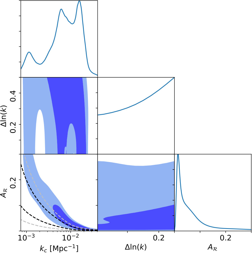 Figure 1
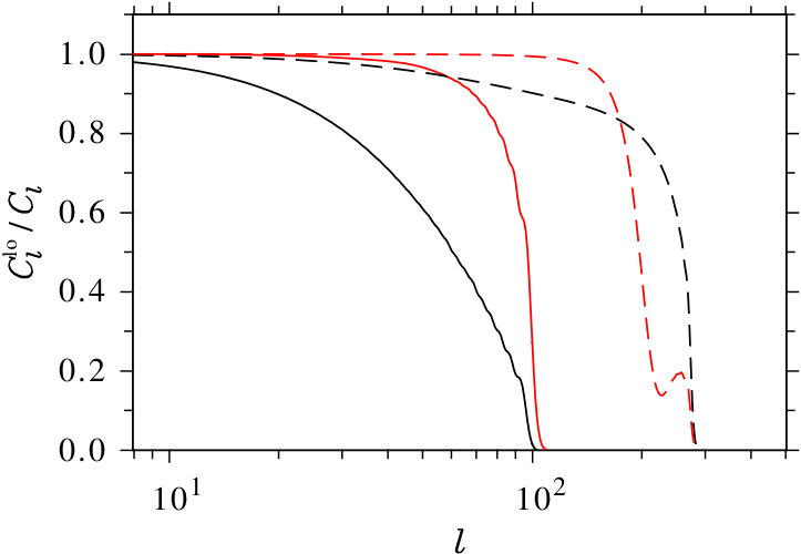 Figure 2
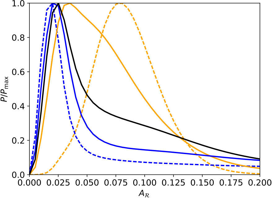 Figure 3
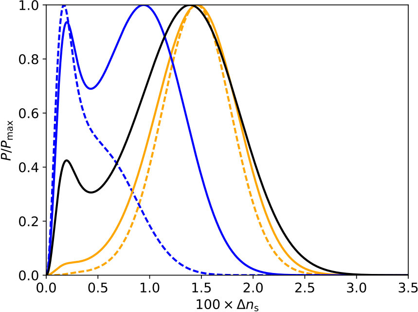 Figure 4
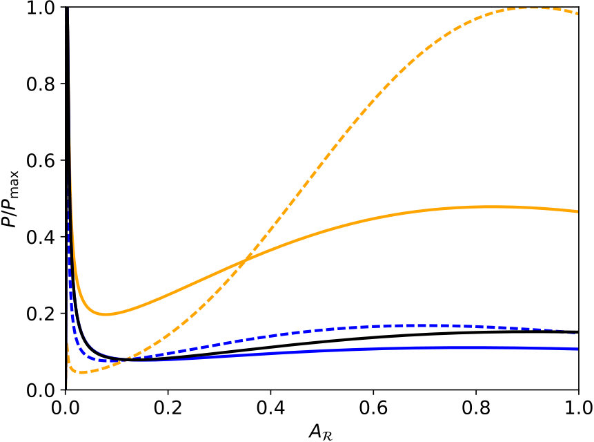 Figure 5
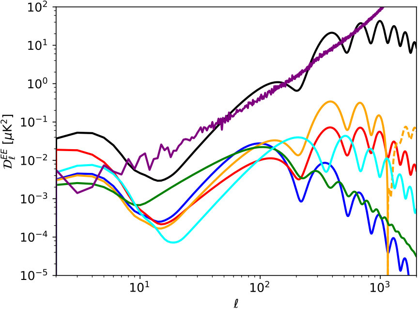 Figure 6
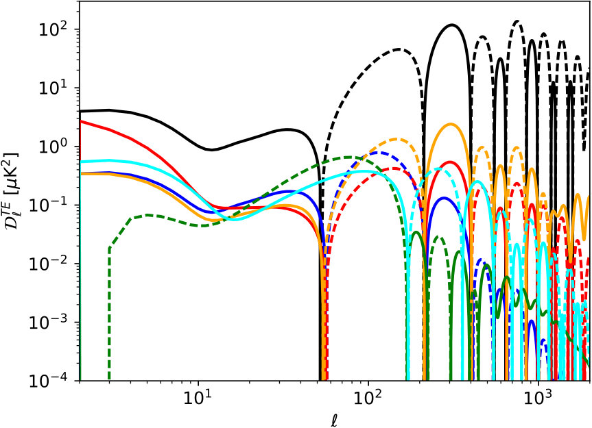 Figure 7
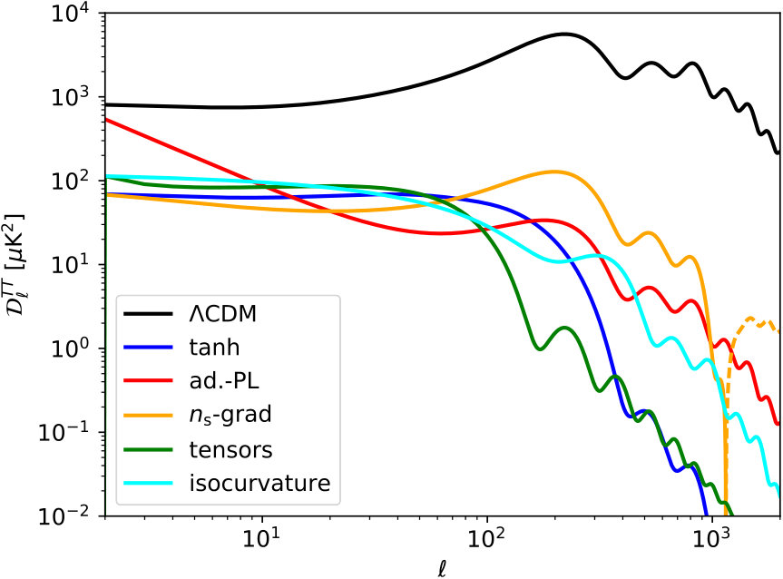 Figure 8
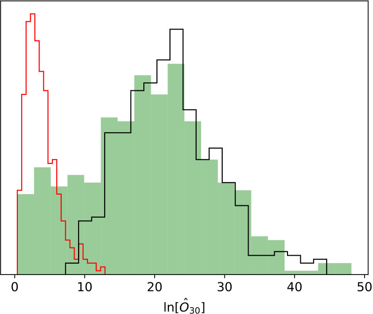 Figure 9
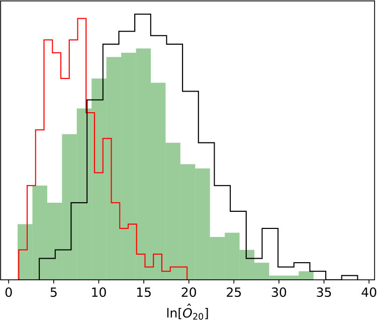 Figure 10
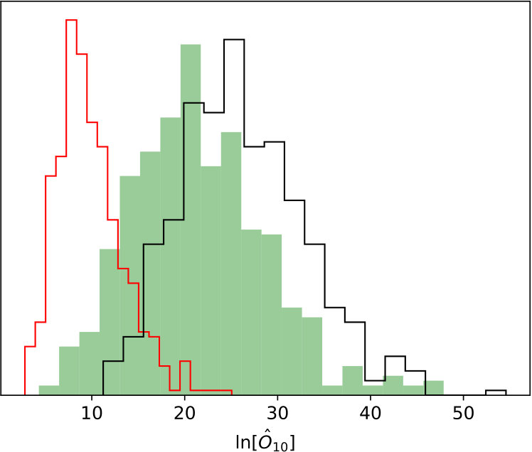 Figure 11
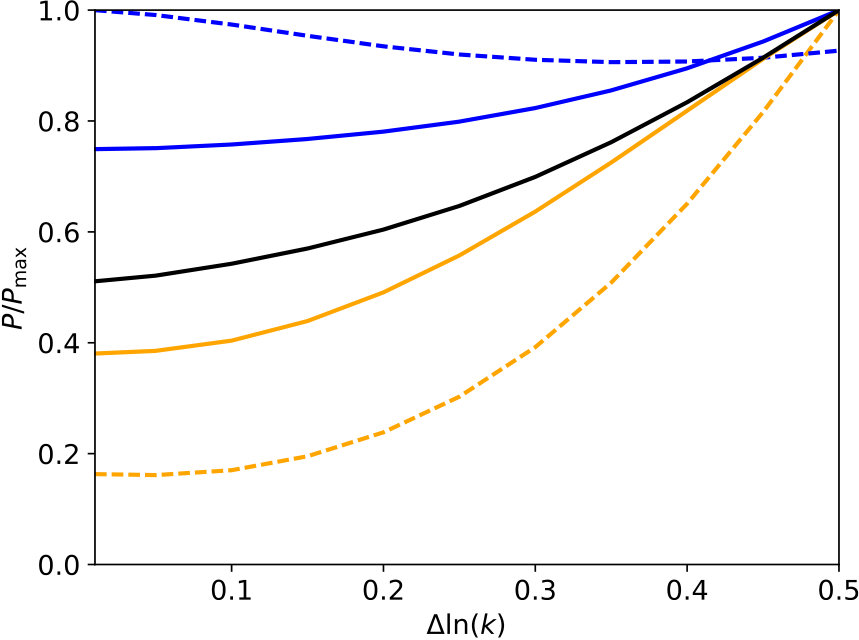 Figure 12
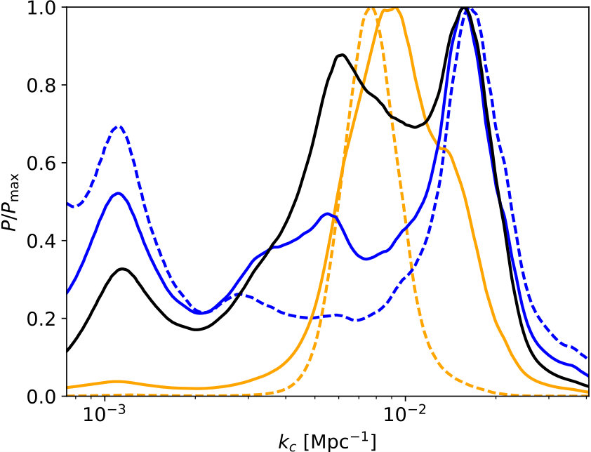 Figure 13
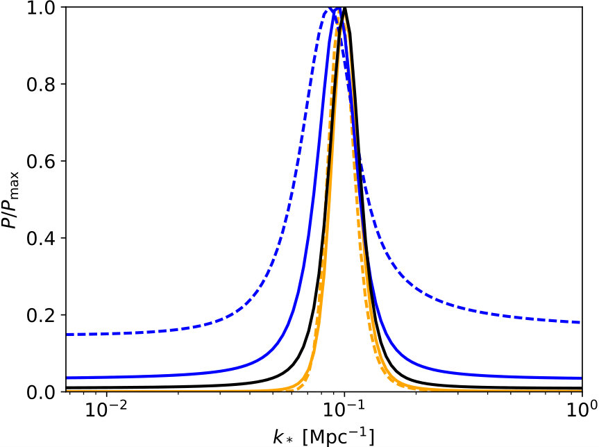 Figure 14
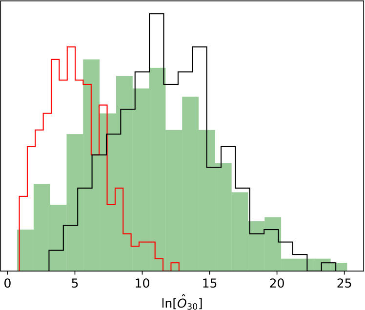 Figure 15
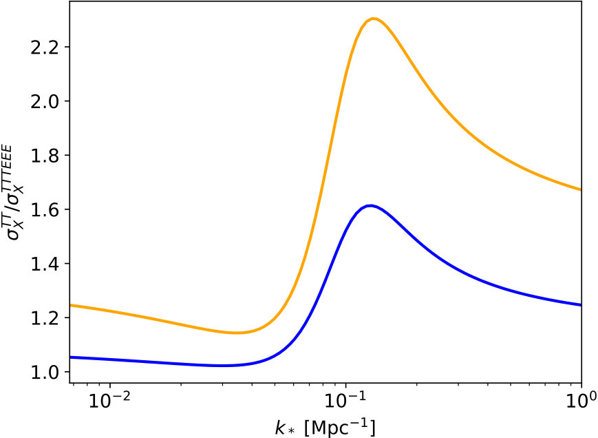 Figure 16
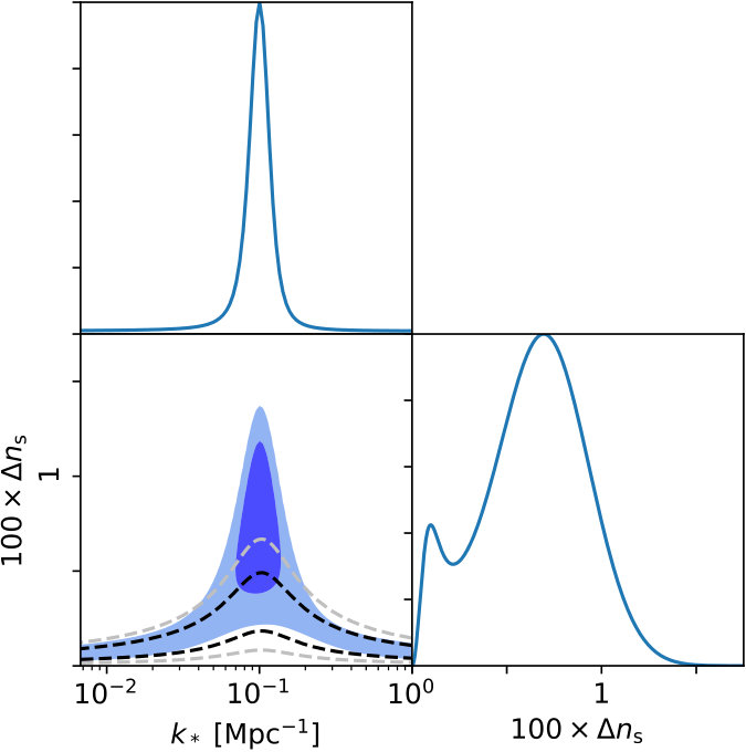 Figure 17
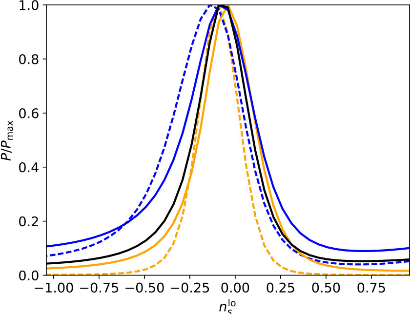 Figure 18
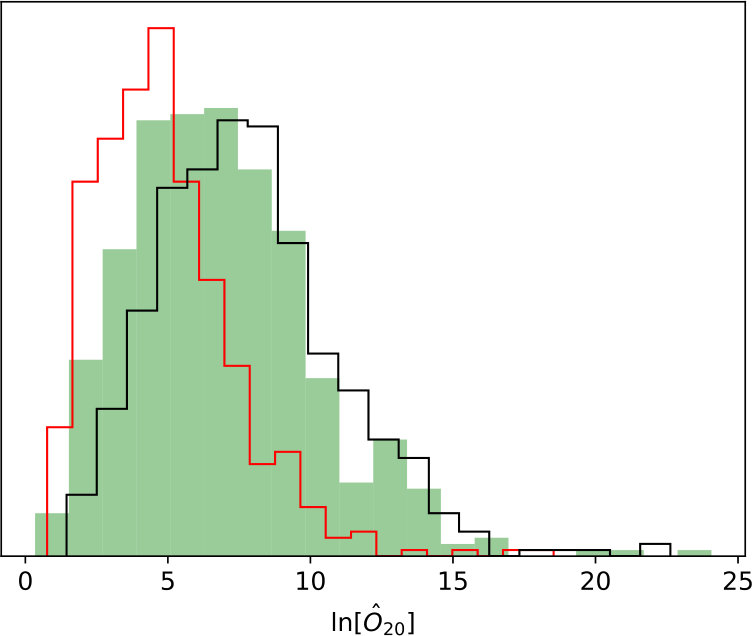 Figure 19
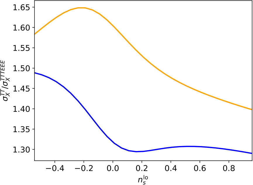 Figure 20
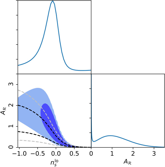 Figure 21
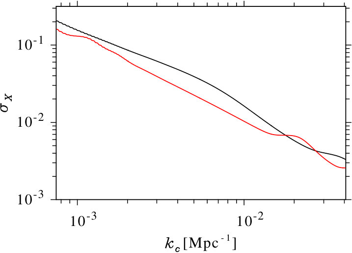 Figure 22
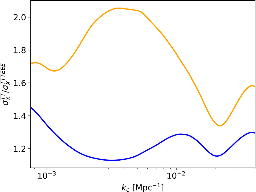 Figure 23
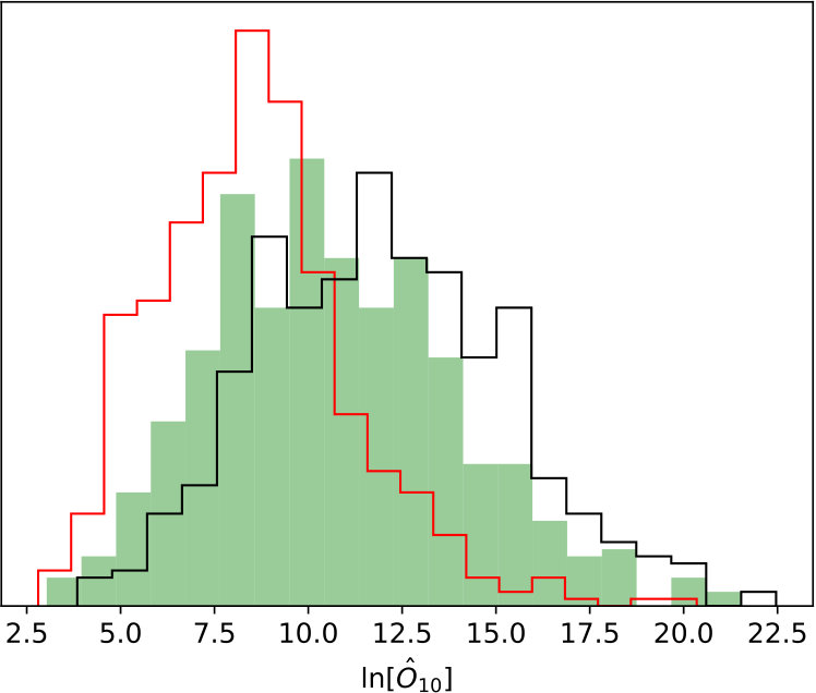 Figure 24
| Parameter | ad.-PL | -grad | tensors | isocurvature | |
|---|---|---|---|---|---|
| Model | Planck | CV-limited | ||
|---|---|---|---|---|
| best fit | sampling | best fit | sampling | |
| 37% | 23% | 94% | 75% | |
| ad.-PL | 27% | 20% | 63% | 45% |
| -grad | 75% | 58% | 99% | 84% |
Peer Reviews
No public reviews on file for this paper yet. If you reviewed it on a platform where reviews are public (OpenReview, ICLR, NeurIPS, ICML), you can paste yours below so the community can read it here.
Videos
No videos yet. Explain this paper in a talk, walkthrough, or lecture? Add one.
Testing physical models for dipolar asymmetry with CMB polarization
D. Contreras
Department of Physics & Astronomy
University of British Columbia, Vancouver, BC, V6T 1Z1 Canada
J. P. Zibin
Department of Physics & Astronomy
University of British Columbia, Vancouver, BC, V6T 1Z1 Canada
D. Scott
Department of Physics & Astronomy
University of British Columbia, Vancouver, BC, V6T 1Z1 Canada
A. J. Banday
Université de Toulouse
UPS-OMP, IRAP, F-31028 Toulouse cedex 4, France
CNRS, IRAP
9 Av. colonel Roche, BP 44346, F-31-28 Toulouse cedex 4, France
K. M. Górski
Jet Propulsion Laboratory, California Institute of Technology
4800 Oak Grove Drive, Pasadena, California, U.S.A
Warsaw University Observatory
Aleje Ujazdowskie 4, 00-478 Warszawa, Poland
Abstract
The cosmic microwave background (CMB) temperature anisotropies exhibit a large-scale dipolar power asymmetry. To determine whether this is due to a real, physical modulation or is simply a large statistical fluctuation requires the measurement of new modes. Here we forecast how well CMB polarization data from Planck and future experiments will be able to confirm or constrain physical models for modulation. Fitting several such models to the Planck temperature data allows us to provide predictions for polarization asymmetry. While for some models and parameters Planck polarization will decrease error bars on the modulation amplitude by only a small percentage, we show, importantly, that cosmic-variance-limited (and in some cases even Planck) polarization data can decrease the errors by considerably better than the expectation of based on simple -space arguments. We project that if the primordial fluctuations are truly modulated (with parameters as indicated by Planck temperature data) then Planck will be able to make a 2 detection of the modulation model with 20–75% probability, increasing to 45–99% when cosmic-variance-limited polarization is considered. We stress that these results are quite model dependent. Cosmic variance in temperature is important: combining statistically isotropic polarization with temperature data will spuriously increase the significance of the temperature signal with 30% probability for Planck.
I Introduction
The largest scales of our cosmic microwave background (CMB) temperature sky exhibit a dipolar asymmetry with an amplitude at the percent level Eriksen et al. (2004); Hanson and Lewis (2009); Bennett et al. (2011); Ade et al. (2014a, 2016a). While the cosmological origin of this signal is not in dispute (existing in both WMAP and Planck data with very different systematic effects and frequency coverage), its statistical significance is debated (see Bennett et al. (2011); Ade et al. (2016a) and references therein). Without correction for the effects of a posteriori selection, this large-scale signal has a significance at approximately the level and an amplitude of roughly 6–7%, when restricted to a multipole range of . Applying look-elsewhere correction on the maximum multipole reduces the corresponding -value to of order 10% Bennett et al. (2011); Ade et al. (2016a). However, the asymmetry is present on scales that are roughly super-Hubble at last scattering, suggesting a possible physical origin related to very-early-Universe physics. If this were the case, the former significance estimate might be more relevant given a model that predicted it.
The dipolar asymmetry in temperature is now characterized as well as it ever will be, because the measurements on these scales are limited by cosmic variance and hence essentially all the cosmological information has already been extracted. The only way to unambiguously determine if this signal is due to a physical modulation of fluctuations or is just a random statistical fluctuation is to acquire new information (i.e., measure new and independent modes Scott et al. (2016)). This can be achieved with the addition of large-scale polarization data. Polarization data are available from the Planck satellite; however, residual systematics (particularly at large angular scales) have so far prevented a full investigation of the polarization dipole asymmetry signal. Other probes of new modes that have been examined in this context include large-scale structure Hirata (2009); Fern ndez-Cobos et al. (2014); Yoon et al. (2014); Baghram et al. (2014), CMB lensing Zibin and Contreras (2017); Hassani et al. (2016), cm measurements Shiraishi et al. (2016), and spectral distortions Dai et al. (2013).
The use of polarization in the investigation of dipole asymmetry has been examined previously in Refs. Dvorkin et al. (2008); Paci et al. (2010); Chang and Wang (2013); Paci et al. (2013); Dai et al. (2013); Ghosh et al. (2016a); Kothari et al. (2016); Kothari (2015); Namjoo et al. (2015); Bunn et al. (2016). In particular, it was appreciated Dvorkin et al. (2008); Namjoo et al. (2015) that a modulation model must be constructed in position (or ) space and propagated to map (or spherical harmonic) space in order to consistently describe both temperature and polarization modes. In addition, it was found that the predicted signature in polarization is quite dependent on the assumed model for the -space modulation Namjoo et al. (2015). Here we will use the temperature data to predict the polarization signature given a -space modulation model, following the formalism developed in Ref. Zibin and Contreras (2017).
Naively, one might expect that the temperature signal, together with the assumption of a physical modulation of the large-scale three-dimensional fluctuation field, would predict a roughly 6–7% asymmetry in polarization in the range of 2 to 65. However, this is not necessarily the case, since the mapping (transfer functions) from to space differs between temperature and polarization. Therefore, in the absence of a detailed physical modulation model we cannot use polarization to test for such a physical origin. In addition, as stressed in Ref. Zibin and Contreras (2017), the signal in the temperature data alone is not strong enough to pick out a well-defined modulation scale dependence. In this paper we will explore how these issues are modified with the inclusion of polarization data in more detail.
One well-known concern when considering polarization is the correlation between temperature and gradient- (or -) mode polarization. More specifically, modes we can measure from polarization are not completely independent of temperature. This correlation may alter a possible polarization asymmetry signal or mimic such a signal in its absence. We deal with the correlation by calibrating our estimator on Planck Full Focal Plane (FFP8) temperature and polarization simulations Ade et al. (2016b) that are appropriately correlated. A further concern is the spurious enhancement of a modulation signal when including polarization. That is, simply due to cosmic variance and noise, adding polarization to temperature might sometimes increase the significance of a signal even when there is no true underlying modulation. This is especially true when the original temperature signal is of low to moderate significance, as is the case with our real CMB sky. We address this concern by quantifying the expected effect of adding polarization both with and without an underlying physical modulation.
Our main goals are to determine how likely it is that a physical origin for a modulation could be confirmed or refuted, and to quantify the expected improvement in constraints on the -space modulation model parameters, with the addition of polarization data. We will present projections for Planck as well as a cosmic-variance-limited polarization measurement. We will not perform a blind multipole-space dipole asymmetry search as has been done with temperature, though this can be done with the estimator we employ here and will be important to perform once the data are available.
For this study we use the FFP8 cosmological parameters, with Hubble parameter , where , baryon density , cold dark matter (CDM) density , neutrino density , cosmological constant density parameter , primordial comoving curvature perturbation power spectrum amplitude (at pivot scale ) and tilt , and optical depth to reionization .
Note that at high our results would be biased due to the effect of aberration Aghanim et al. (2014), which is not present in the FFP8 simulations Ade et al. (2016b). In Appendix D we describe how we detect aberration in the temperature data and remove it so as not to bias our results.
II Modulation approach
II.1 Formalism
Our goal is to construct position- or -space models that generate scale-dependent dipolar asymmetry, while remaining agnostic as to the detailed origin (presumably inflationary) of the modulation. Based on the temperature signal, we would like to modulate the largest scales while maintaining consistency with the usual isotropic CDM power spectra. We consider three different types of model: the first is a modulated adiabatic mode which comprises a part of the total primordial power spectrum 111One particularly motivated model of this form would be a modulated integrated Sachs-Wolfe component, which will be examined in Contreras et al. (2017).; the second is a modulated CDM isocurvature mode; and the third is a modulated tensor mode 222We note that a modulation of the optical depth to reionization Dai et al. (2013) is likely extremely disfavoured since it would imply temperature asymmetry to the smallest scales, contrary to the observations Hansen et al. (2009); Hanson and Lewis (2009); Flender and Hotchkiss (2013); Ade et al. (2016a); Quartin and Notari (2015); Aiola et al. (2015).. For the adiabatic scalar case, we must modulate a large-scale part of the spectrum. The contributions from CDM isocurvature and tensor modes, however, are naturally restricted to scales (at least for near-scale-invariant spectra). Therefore in these cases we only need to apply a scale-invariant modulation to the tensor or isocurvature component. We will analyze each of these models with a slight generalization of the approach in Zibin and Contreras (2017), which considered only the adiabatic scalar case, and we refer to that reference for full details. Our approach will be readily applicable to other modulation models.
We begin by decomposing the primordial fluctuations into two components. The first, , is spatially linearly modulated, and hence its intersection with our last-scattering surface will be dipole modulated. It takes the form
[TABLE]
where is statistically isotropic with power spectrum , is the modulation amplitude, is the direction of modulation, and is the comoving distance to last scattering. The second, unmodulated component, , is statistically isotropic with power spectrum . The two fields are uncorrelated, i.e.,
[TABLE]
The field will correspond to the isocurvature, tensor, or modulated adiabatic component, while will be the remaining, unmodulated adiabatic component. The superscripts “lo” and “hi” refer to the fact that generally these components will dominate at low and high , respectively. Strictly, we should consider only amplitudes , since for larger the fluctuations in Eq. (1) will vanish somewhere inside the last scattering surface and the details in this case may depend on the specific (presumably inflationary) realization of the model.
As shown in Ref. Zibin and Contreras (2017), the total temperature anisotropies will be given to very good approximation by the sum of the uncorrelated contributions from the modulated and unmodulated fluctuations, i.e.,
[TABLE]
The anisotropies , with power spectrum , are generated by the perturbations with power spectrum , while , with spectrum , are generated by the uncorrelated perturbations with power spectrum . The form of Eq. (3) is easy to understand in the limit where the anisotropies are much smaller than the length scale of modulation (i.e., ). The large-scale case is less obvious, but Eq. (3) still holds to very good approximation Zibin and Contreras (2017). We have ignored the ISW effect here, since it would introduce a negligible modification Zibin and Contreras (2017).
For the -mode polarization anisotropies, we similarly use
[TABLE]
Due to the effects of reionization and the non-local definition of modes, Eq. (4) becomes inaccurate on the very largest scales, . In Appendix A, we derive the effect of a spatially linear modulation on the (and ) modes, taking the non-locality into effect. We find that omiting this correction results in a bias to our recovered modulation amplitudes of roughly in the worst case (the most red-tilted power law model we consider). Hence we do not apply this correction here (but plan to implement it in future work). In Appendix A, we also show that the correct treatment results in novel couplings between modes and or modes for a linear modulation. The very-large-scale nature of the corrections implies weak statistical weight, but these unusual couplings could in principle be used to constrain large-scale signals.
In terms of spherical harmonic coefficients, the total fluctuations in Eqs. (3) or (4) can be written as
[TABLE]
where are the statistically isotropic modes, and the are the spherical harmonic decomposition of (the dipolar nature ensures that ). The are coupling coefficients defined by
[TABLE]
and given explicitly by
[TABLE]
where
[TABLE]
From Eq. (5) we can find the covariance of the total temperature or polarization anisotropy multipoles to first order in the modulation amplitude :
[TABLE]
where . The above equation explicitly shows that a dipole modulation will lead to coupling of to modes in the multipole covariance Prunet et al. (2005). In Eq. (12) is the the total isotropic power spectrum, which, since the two fluctuation components are uncorrelated, is given to linear order in the asymmetry by
[TABLE]
and similarly for polarization. Clearly, must be consistent with measurements of the isotropic power. For the adiabatic cases, we take
[TABLE]
where
[TABLE]
is the comoving curvature power spectrum for CDM, so that the isotropic power constraints are automatically satisfied. However, constraints on isocurvature and tensor isotropic contributions Ade et al. (2016c, 2015, d) should be incorporated in addition to the constraints from the temperature asymmetry in order to obtain the tightest constraints for those models Contreras et al. (2017).
II.2 Adiabatic modulation
II.2.1 spectrum
For scalar adiabatic modes Zibin and Contreras (2017) the fluctuation fields and both correspond to the comoving curvature perturbation, . Our first specific model is intended to capture a large-scale modulation with a small number of parameters. We choose a modulated component spectrum of the form
[TABLE]
This smooth step function in ensures that mainly the largest scales, , are modulated. The quantity determines the sharpness of the transition from modulated to unmodulated scales. The other parameters of the model are the amplitude of modulation () and its direction () in Galactic coordinates. The unmodulated contribution is fixed by Eq. (14). It must be noted that the temperature data alone are not strong enough to constrain all five modulation parameters (); see Ref. Zibin and Contreras (2017). The shapes of the best-fit asymmetry spectra for the model (and all of the others) will be illustrated in Sec. IV.1.
As shown in detail in Zibin and Contreras (2017), the fact that we have split the adiabatic fluctuations into two uncorrelated parts does not restrict the modulation mechanism (presumably inflationary) in any way. Instead this is a convenient way to describe an adiabatic spectrum modulated with arbitrary scale dependence.
II.2.2 Power-law spectrum
The modulation model in Eq. (16) is not explicitly motivated by any early-Universe model. Perhaps better motivated would be a simple power-law modulation, i.e.,
[TABLE]
where is the tilt and is the pivot scale of the modulated component of fluctuations. This model will be abbreviated “ad.-PL”. We again impose Eq. (14) in order to define the unmodulated . We consider only red tilts with , and choose , which corresponds roughly to quadrupolar angular scales. Larger would contradict the positivity of on the largest observable scales, while smaller would be degenerate with the modulation amplitude. Again we modulate with amplitude , so the total modulation fraction approaches on large angular scales. This model also should be taken with some caution, since for large departures from scale invariance (i.e., ), we might expect higher-order terms such as running, running of running, etc. in the modulation spectrum.
II.2.3 Modulated scalar spectral index
Next we consider a single-component adiabatic model with a linear gradient in the tilt, , of the primordial power spectrum Moss et al. (2011). We abbreviate this model “-grad”. In this case we do not strictly follow the two-component formalism of Sec. II.1, but instead can directly write the asymmetry spectrum as Moss et al. (2011)
[TABLE]
Here we have used a linear approximation for the effect of the gradient, which will be well justified by our results. We allow for free modulation amplitude, , and let the tilt pivot scale, , vary. Note that this treatment is degenerate with fixed pivot and additional modulation of the primordial amplitude, . Since a modulation of tilt produces extra power on large scales in the direction, we have included a minus sign in Eq. (18) so that the best-fit modulation directions will be directly comparable to those of the other models.
II.3 Tensor modulation
The possibility that a modulated tensor component is present is particularly well motivated observationally Dai et al. (2013); Scott and Frolop (2014); Chluba et al. (2014), since the contribution of (near-scale-invariant or red-tilted) tensors is negligible at small scales. Tight constraints on the tensor-to-scalar ratio will make it difficult to achieve sufficient modulation, however, via the isotropic power constraint Chluba et al. (2014); Contreras et al. (2017).
In this case we take the unmodulated component to be adiabatic fluctuations with the standard CDM form, Eq. (15). The modulated component will be a scale-invariant tensor contribution, i.e.,
[TABLE]
with (this is the 95% upper limit from Ade et al. (2016d)) at pivot scale Mpc*-1*. The tensor modes are uncorrelated with the adiabatic fluctuations (note that even in the presence of such correlations, the scalar and tensor anisotropy power spectra would still be additive Zibin (2014)) and modulated in a scale-invariant way with amplitude . As before, the tensors produce anisotropy power (and similarly for ).
II.4 Isocurvature modulation
Also well motivated as a modulation model is the CDM isocurvature spectrum, since it naturally contributes mainly at large angular scales for near-scale-invariant (or red-tilted) isocurvature modes Erickcek et al. (2009). In this case we assume that the unmodulated is an adiabatic contribution which takes the standard, CDM form, Eq. (15). The modulated part will be the isocurvature component, which we take to be scale-invariant, i.e.,
[TABLE]
where we use the same pivot scale as for the tensors. The isocurvature modes are taken to be uncorrelated with the adiabatic fluctuations and modulated in a scale-invariant way with amplitude . This isocurvature spectrum then determines the modulated component of the CMB fluctuations, . The isocurvature fraction, , should properly be constrained by the isotropic Planck likelihood Contreras et al. (2017), but here we simply choose the Planck upper limit for uncorrelated, scale-invariant isocurvature, Ade et al. (2016c).
III Dipole asymmetry estimator
In this section we describe the estimator that we use to extract modulation parameters from data or simulations given a modulation model. This estimator is applied in harmonic space, exploiting the fact that (to leading order in the anisotropy) dipole modulation is equivalent to the coupling of with modes, as we saw in Sec. II.1.
III.1 Connection to previous approaches
The estimator that we use was originally developed for temperature data Moss et al. (2011); Ade et al. (2016a); Zibin and Contreras (2017), but can equally be applied to polarization (subject to the caveats discussed in Sec. II.1). Our current implementation includes new improvements to the treatment compared with Ade et al. (2016a); Zibin and Contreras (2017) in order to account for the expectation of noisy polarization data. Differences in the implementation of the estimator between this work and Ref. Zibin and Contreras (2017) are outlined in Appendix B, while the consequent differences in temperature results can be seen by comparing Table 1 with table I of Ref. Zibin and Contreras (2017) (though the differences are not significant). Here we present a condensed description of our estimator (the full details are in Appendix C of Ade et al. (2016a)).
We note that our estimator is essentially identical to that of Ref. Hanson and Lewis (2009) and can also be rewritten in terms of BiPoSH coefficients Hajian and Souradeep (2003, 2006); however, the physical motivation for this approach comes from Ref. Moss et al. (2011), where general cosmological parameter modulations were explored. Our implementation to deal with masking and noise uses an inverse-variance filter on the spherical harmonic coefficients that optimally account for the masking, as used in Refs. Ade et al. (2014b, 2016e, 2016a).
III.2 Full-sky, noise-free case
From Eq. (12) it is clear that the multipole covariance can be decomposed into an isotropic part and a small anisotropic part proportional to . In other words, we can make the identification , with being the first term on the right-hand side of Eq. (12) and being the second term. The inverse covariance matrix can then be written as (to linear order in the anisotropy). The best-fit values are given by
[TABLE]
for multipole vector . These can be written more explicitly as
[TABLE]
and . We note that Eq. (21) is completely general and can be used to examine modulation of any kind (i.e., beyond simple dipolar modulation). The cosmic variance of the modulation amplitude estimator is given by
[TABLE]
As we mentioned in Sec. II.1, we strictly only consider values of the modulation amplitude (, , , or ) less than unity. Note, however, that the terms which were dropped in the multipole covariance, Eq. (12), couple with and . Therefore the estimator, Eqs. (22) and (23), will be insensitive to them. In other words, our approach will recover modulation amplitudes as large as unity without bias: we have no need to restrict to small . However, the results will not be optimal, and could be improved for large by incorporating these extra couplings into the estimator.
III.3 Realistic skies
The estimators presented in Sec. III.2 are only adequate for full sky coverage with no noise. In this subsection we show how we include the effects of masking and noise in the data.
The combination of in Eq. (21) is suggestive that we should apply an inverse-covariance filter to the data. This is exactly what we do. The effects of masking are readily dealt with by employing inverse-variance filtering to the data, as described in Refs. Ade et al. (2014b, 2016e). Pixels within the mask are given infinite variance and thus are given zero weight, which optimally accounts for masking effects. The effects of inhomogeneous noise could also readily be handled by including its variance contribution in the inverse-variance filter. However, we have not included these effects, which means we will have a slightly suboptimal though still unbiased estimate. Residual effects not captured by our approach (e.g. inhomogeneous noise) are handled by subtracting a mean field term, derived from simulations with the same foreground and noise properties as the data. We note that this same approach has been used for lensing estimators in Refs. Ade et al. (2014b, 2016e) and specifically for temperature dipole modulation in Refs. Ade et al. (2016a); Zibin and Contreras (2017). Cut-sky aberration effects Jeong et al. (2014) are taken into account by removing aberration from the data as described in Appendix D.
The estimator, Eqs. (22)–(23), then becomes
[TABLE]
with
[TABLE]
Here, ; and are inverse-covariance filtered data; ; and the last term on the right-hand-side of Eq. (27) denotes the mean-field correction (details including the precise form of can be found in Appendix A.1 of Ref. Ade et al. (2016e) and Appendix B of this paper). The parentheses in the superscripts indicate symmetrization over the enclosed variables.
The estimators of Eqs. (25)–(26) can be combined with inverse-variance weighting over all data combinations (, , ) to obtain a combined minimum-variance estimator, given by
[TABLE]
Here we calculate the variance from the scatter of simulations, although they agree closely with the Fisher errors given in Ref. Ade et al. (2016a).
IV Results
IV.1 Temperature only
In this section we present constraints using Planck temperature data only. Specifically, we use the SMICA 2015 temperature solution, one of four Planck component-separation methods Adam et al. (2016a), all of which produce very similar results Ade et al. (2016a). The temperature data are evaluated up to a maximum multipole (no significant difference was found when extending to higher multipoles), with the exception of the modulated model, which uses .
Fig. 1 shows the posteriors of the modulation parameters for our adiabatic models. Results for the model have already been commented on in Zibin and Contreras (2017); here we simply reiterate that the model is (unsurprisingly) not constrained well with temperature alone. The pile-up of the posterior at low modulation amplitudes (present for all models, though most notably for the adiabatic power-law model) is a volume effect that arises due to our choice of prior, which expects uniform posteriors for the -space parameters () for statistically isotropic data.
The best-fit modulation parameters for all models are presented in Table 1. We see that the modulation amplitudes required for the tensor and isocurvature models exceed unity, i.e., the best fits have . This suggests that, for the case of tensor and isocurvature isotropic contributions at the current upper limits ( and ), maximal modulation (i.e., modulation amplitude unity) is insufficient to produce the observed temperature asymmetry. For this reason we do not discuss these models further here. This result will be addressed more quantitatively in Contreras et al. (2017). Note that this conclusion for a specific isocurvature model was originally made in Ade et al. (2016c) and the difficulty of providing sufficient modulation for tensor models was discussed in Dai et al. (2013); Scott and Frolop (2014); Chluba et al. (2014). Furthermore, the best-fit value of for the -grad model is tighter than the corresponding value of in Dai et al. (2013). This illustrates the constraining power of the small-scale anisotropies in our analysis.
In Fig. 2 we compare the CDM power spectra to the asymmetry spectra, , for the temperature best-fit modulation parameters given in Table 1, for each of our models. Note that the best-fit asymmetry spectra correspond very roughly to modulation in amplitude out to , as expected from the previous -space analyses of the asymmetry.
It is worth reiterating that none of these models are currently favoured over base CDM: the goodness of fit of these models to the asymmetry (and isotropic) data is discussed in detail in Contreras et al. (2017). Hence the interest here in pursuing polarization data to improve constraints and test for a physical origin to the asymmetry.
IV.2 Including polarization
IV.2.1 vs. asymmetry spectra
We claimed in Sec. I that it was not reasonable to take the observed multipole-space temperature asymmetry, e.g., asymmetry to , and predict a asymmetry in to . We demonstrate this explicitly in this subsection, using the model as an example. First, in Fig. 3 we illustrate the cosmic variance [calculated via Eq. (24)] for a measurement of the amplitude of modulation versus cutoff scale , for (which corresponds closely to a step function in -space, with modulation only for ). It is clear that for most values of , the cosmic variance is considerably smaller for an measurement than for a measurement. In particular, this applies around the best-fit value, Mpc*-1*, where the standard deviation is smaller by a factor of nearly two than the value. This is in stark contrast to the naive -space expectation, where identical modulation cutoffs for and leads to identical cosmic variance. However, we can also see that there are some values of for which the cosmic variance is comparable to or even worse than the value.
To help understand these differences between and , we plot in Fig. 4 asymmetry spectra and for the model with . For the case (i.e., the best-fit value), we can see that the asymmetry spectra differ substantially between and (note that this effect is also visible in figure 1 of Namjoo et al. (2015)). In particular, we predict substantially larger modulation, and hence lower cosmic variance, in than in , since for all . The reason is that the transfer functions from - to -space are narrower for than for , and hence the step in -space is better resolved in . On the other hand, for the case some fine -space structure (a dip in this case) is resolved by polarization and leads to lower asymmetry power for and hence larger cosmic variance. This illustrates the necessity of working in -space rather than -space when testing physical models for modulation.
Importantly, these results imply that an ideal polarization measurement can improve on the modulation amplitude measurement error considerably better than the naive -space expectation of . In Fig. 5 we show the expected improvement to the error bar on the amplitude of modulation in a known direction () when adding Planck or cosmic-variance-limited polarization to Planck temperature, as a function of the modulation parameters. (Recall that for temperature we use for the gradient model and for all others.) For the model the dependence on is quite weak and so we have averaged over it and only show the dependence on . We can see that even with Planck polarization (blue curves), there are parameter values for which the addition of polarization decreases the error bar by more than the naive expectation of . This, again, is due to the difference in the -to- transfer functions between polarization and temperature. That is, for the same modulation, polarization modes are more strongly modulated (on many scales) than temperature, as we saw in Fig. 4. It is also worth noting that the variations in improvement follow the peak structure of the power spectra, i.e., the first three peaks that are above the noise level in Fig. 2. This is most clearly evident with the model. The expected improvement when adding cosmic-variance-limited polarization exceeds a factor of two for some models and parameter ranges, substantially exceeding the naive value of .
IV.2.2 Constraints
We cross-check and validate our method through the use of FFP8 component-separated CMB + noise simulations Ade et al. (2016b), masked appropriately using the Planck 2015 common mask for polarization, with unmasked fraction . For our cosmic-variance-limited results we remove the noise in the polarization simulations and apply no mask. For all models we examine our polarization simulations up to a maximum multipole . Throughout we will consider adding statistically isotropic or anisotropic polarization to Planck temperature data. In both scenarios we will use the same set of FFP8 simulations, modified to either include the appropriate temperature-polarization correlation with the given temperature data (for the case of statistically isotropic polarization, see Appendix C.1), or to include the appropriate modulation for the specific model and parameters considered (see Appendix C.2).
First we consider the case that the asymmetry does not have a physical origin and is simply the result of fluctuations due to cosmic variance. In this case the polarization must be treated as statistically isotropic (apart from the necessary - correlation). We apply Bayesian parameter fitting to the combination of temperature data and polarization simulations (treated as if they were data). In Figs. 6–8 we show the marginalized posteriors of the modulation parameters for temperature data alone (in black) and when adding statistically isotropic polarization data averaged over 500 simulations and shown by the blue solid and dashed curves for Planck and cosmic-variance-limited polarization, respectively. In general the addition of isotropic polarization data will act to spread out the posteriors with respect to the temperature-only constraints. However, we find that the addition of statistically isotropic polarization data increases the significance of a temperature result (here we mean with respect to the amplitude parameter only) roughly 30% or 20% of the time for Planck or cosmic-variance-limited polarization, respectively (for the model). This is mainly due to the initial weakness of the temperature signal. Therefore, we urge caution when interpreting the addition of polarization data to temperature.
Next we consider the case that the asymmetry is due to a real modulation, so the polarization will be statistically anisotropic with a precise form determined by the -space modulation model. We generate modulated polarization simulations (modulated with the temperature best-fit parameters given in Table 1) to combine with the temperature data to forecast the type of constraints we expect to see in Planck and cosmic-variance-limited data if the modulation is real. We modify the existing FFP8 simulations following the procedure in Appendix C.2.
Results are also summarized in Figs. 6–8, where the addition of modulated polarization is shown with the orange solid and dashed curves for Planck and cosmic-variance-limited polarization, respectively. The curves plotted are the mean posteriors averaged over 500 simulations. We see that in general the addition of polarization makes the data more constraining. However, these figures do not show how often we should expect to be able to distinguish modulated polarization from statistically isotropic polarization, which will necessarily be model dependent. We will be more quantitative about this in the following subsection.
IV.3 Distinguishing modulated from isotropic polarization
If the signal seen in temperature has a physical cause then it is clearly too low in signal-to-noise to definitively distinguish from cosmic variance fluctuations. With the addition of polarization, however, we can assess how well one could distinguish statistically anisotropic from statistically isotropic data. With this in mind we define the quantity as the ratio of the maximum likelihood of model to that of model . For definiteness we will order the models in the following way:
CDM; 2. 1.
model; 3. 2.
adiabatic power-law model; 4. 3.
gradient.
For a modulation model , the maximum likelihood is proportional to , whereas for CDM, it is proportional to . Therefore we can compute as
[TABLE]
Note that Eq. (29) is related to the often used odds ratio for Bayesian model comparison, but without the Occam penalty factor Gregory (2005). For this reason the meaning of the absolute value of is irrelevant, though the relative value between different data (modulated or statistically isotropic) is valuable. We will thus use as a proxy for distinguishing modulated data from statistically isotropic data by comparing to statistically isotropic or modulated simulations.
For the data we will choose to add either statistically isotropic or modulated polarization to the existing Planck temperature data. The results are shown in Figs. 9–11, where the relation between the colours and the type of simulations are as follows: {labeling}simulations
statistically isotropic polarization added to temperature data;
modulated polarization added to temperature data, where the modulation parameters are determined by randomly sampling the full likelihood of the temperature data;
modulated polarization added to temperature data using the best-fit modulation parameters from Table 1.
The figures show the histogram of the logarithm of . Large values of relative to the isotropic-polarization simulations indicate that the modulation model should be preferred over CDM, and indeed the modulated simulations are clearly shifted to the right of the statistically isotropic simulations, with the black histograms further to the right than the green. A large overlap in the distributions would indicate that it will be difficult to distinguish modulated from statistically isotropic data using polarization.
We would like to assess the probability of a detection of modulation assuming that the polarization data are modulated as predicted by temperature. In Table 2 we indicate for each model the probability that is greater than that of 95% of isotropic (red) simulations—we will loosely refer to this as a “”-detection. The “best-fit” values refer to polarization modulated with the temperature best-fit parameters from Table 1. In this case the probability of a detection with Planck polarization ranges from for the adiabatic power-law model to for the gradient model. For cosmic-variance-limited polarization these probabilities increase substantially, reaching for the gradient model. However, as the “sampling” columns in Table 2 show, when we sample the modulation parameters from the full temperature posteriors, the probabilities are reduced.
We see that even in the optimistic scenario that the true modulation parameters are given by the best-fit values of the temperature likelihood, Planck has a low probability of distinguishing this from statistically isotropic data. The exception is the case of the gradient model, which has a large tail out to very large values even when simulated Planck polarization data are used. The situation improves considerably when cosmic-variance-limited polarization is used, with the and -grad models being almost guaranteed to be detected in the scenario that the true modulation model is given by the best-fit temperature parameters. These large probabilities are diminished when we consider the case that polarization is instead modulated with parameters randomly sampling the likelihood of the temperature data, which is not constrained well. However, these “sampling” probabilities are the best statements we can make about detectability of modulation given the temperature signal, and should be considered as our most conservative results.
V Discussion
In this paper we have applied to CMB polarization the formalism of Ref. Zibin and Contreras (2017), which describes the effect of a spatially linear modulation with arbitrary scale dependence. We have used the statistically isotropic temperature and polarization simulations provided by the Planck collaboration to estimate the decrease in uncertainty in the modulation parameters when polarization is added. We have also generated asymmetric polarization simulations to see how well we could test the possibility that the modulation is a real, physical effect. We have characterized the probability of a “2” detection of our dipolar modulation models (introduced in Sec. II) when adding Planck or cosmic-variance-limited polarization data under the following important assumptions: 1) The modulation model is correct (i.e., the primordial fluctuations are actually modulated according to the model in question); 2) the polarization data are free of any relevant systematic effects; and 3) the effective sky coverage is similar to what is available for the Planck temperature data (though our noiseless polarization simulations use the full sky). We found that, for the case of Planck polarization, we expect a probability of anywhere from 20% to 75% for such a detection. For cosmic-variance-limited polarization, the probability increases to the range 45% to 99%. We have shown that these results are considerably stronger than a simple -space analysis would predict, due to the ability of polarization to resolve -space detail more sharply than temperature.
Our results are clearly strongly model dependent, with the gradient model being the most likely to be ruled out or confirmed. This is due to the distinct scale dependence for this model, with substantial modulation at very small scales. This suggests that extending the polarization data to would provide a decisive test of this model 333In addition, asymmetry constraints from large-scale structure surveys Gibelyou and Huterer (2012); Fern ndez-Cobos et al. (2014); Baghram et al. (2014); Shiraishi et al. (2017); Zhai and Blanton (2017) should be important for -grad. E.g., for our best-fit parameters, we find a modulation amplitude of about 1.6% at , which is already in strong tension with the 95% upper limit based on quasar data in Hirata (2009)..
Furthermore, we found that the probability that adding statistically isotropic polarization spuriously increases the significance of a signal (with respect to the amplitude) is 30% or 20% for Planck or cosmic-variance-limited polarization, respectively. This probability is large due to the moderate strength of the modulation signal in temperature. Therefore caution is warranted if polarization is found to increase the significance of the temperature signal.
For a spatially linear modulation (as with our models) the addition of polarization is our best short-term hope at detecting such a signal. This is because in practice the surface of last scattering is the furthest distance we have access to and thus perturbations sourced there would be modulated with a higher amplitude than observables such as lensing Zibin and Contreras (2017) or integrated Sachs-Wolfe effect Contreras et al. (2017), for example. In spite of the poor ability of Planck polarization to address modulation, all is not lost, as a CMB-S4 Abazajian et al. (2016) project or CORE Delabrouille et al. (2016) should reach noise levels such that -mode polarization is essentially cosmic-variance limited. This should provide a strong indication of the true nature of the dipole asymmetry signal, at least for some models (recall the final two columns of Table 2). Farther into the future, 21 cm measurements of the dark ages () may be able to help in constraining the dipole modulation models considered here due to the vastly larger number of modes accessible to three-dimensional probes.
Acknowledgements
We thank Jens Chluba for comments on the draft. This research was supported by the Canadian Space Agency and the Natural Sciences and Engineering Research Council of Canada.
Appendix A Dipolar modulation of polarization
In this Appendix we calculate the effect of a spatially linear modulation of the primordial fluctuations on polarization and modes. We will only consider the “lo” component, i.e., the modulated fluctuations. The modulation of the and modes will differ in detail from that of temperature [derived in Zibin and Contreras (2017), and expressed in Eqs. (3) and (5)] due to the nonlocal relation between and and the Stokes and parameters, which, as we will see, are modulated analogously to temperature.
The polarization we see in direction can be written as a line of sight integral in terms of the temperature quadrupole, , seen at scatterer position :
[TABLE]
(see, e.g., Hu (2000)). Here are the spin-2 spherical harmonics and is the optical depth. Importantly, for our purposes we will not need to explicitly calculate the temperature quadrupole; instead, we will only need to know how it is modulated across the sky in the presence of a linear gradient in the primordial fluctuations. The quadrupole at the scatterer will be sourced by the temperature anisotropies at the scatterer’s last-scattering surface. This means that different parts of that source will be modulated by different amounts. However, since the last-scattering surface is much thinner than the distance to last scattering, to very good approximation we can take the quadrupole to be modulated by the amplitude given by the linear gradient evaluated at point . Errors due to this approximation will be of order , where is a characteristic thickness of last scattering. Again, due to the thinness of the last-scattering surface, this approximation will hold independently of the radius of the quadrupole, and so for our purposes we can place the scatterers at one radius () and write the polarization in Eq. (30) as
[TABLE]
where the temperature quadrupole is modulated according to
[TABLE]
In this Appendix, superscript will indicate statistically isotropic and homogeneous fields.
Note that for the reionization bump at the very largest angular scales, , we have . Therefore for polarization sourced at reionization, the error due to the variation of modulation, , will be larger than for polarization from last scattering. Also, for a spatially linear modulation the amplitude of modulation at reionization will be reduced by the factor compared with that in Eq. (32). However, given the low statistical weight for these few very-largest-scale modes, we ignore this effect here. Therefore our approach will slightly overestimate the modulation of the reionization bump.
Combining Eqs. (31) and (32) gives
[TABLE]
In words, the Stokes parameters are simply dipole modulated, just as temperature was in Eq. (3). Again, this approximation will be good for our purposes, i.e., for the sake of quantifying the effect of the modulation on polarization. Note that Eq. (A) was taken as the starting point for polarization modulation in Ghosh et al. (2016b).
The - and -mode multipole moments are defined by
[TABLE]
which implies
[TABLE]
Combining the previous three expressions gives, for the modulated and multipoles,
[TABLE]
where
[TABLE]
generalizes the usual matrix in Eq. (6) to spin-2 fields.
To evaluate the coefficients we can write the spherical harmonics in terms of the rotation matrices Edmonds (1974), with the result
[TABLE]
For the case (i.e., a polar modulation) the non-zero coefficients can therefore be evaluated to be
[TABLE]
[TABLE]
[TABLE]
These expressions agree with those in Ghosh et al. (2016b). Note that (for ), so we expect , coupling in and modes. Also note that are symmetric and is antisymmetric with respect to a sign change of the spin index.
Using these symmetry properties we can now evaluate Eq. (37) for the case of modulation along the polar axis, taking sums and differences to isolate the and modes. The result is
[TABLE]
[TABLE]
These imply
[TABLE]
[TABLE]
[TABLE]
to first order in . The power spectra here are for the isotropic (unmodulated) fields, i.e., etc., but agree with those of the modulated fields to first order in . Using Eq. (5) for the modulated temperature modes, we find
[TABLE]
[TABLE]
also to lowest order in . Note crucially that we find coupling between modes and or modes, which of course vanishes in the statistically isotropic case. However, we have
[TABLE]
since is antisymmetric with respect to .
Appendix B Filtering
In Ref. Zibin and Contreras (2017) a simplified noise model was used when treating the temperature data. The model did not account for variations in the noise level due to the Planck scanning strategy, or scale-dependence of the noise power, or foreground signal. Not accounting for these effects was deemed adequate due to the noise power being subdominant on the scales probed. However, for polarization this is not the case. Here we describe our approach to account for the scale dependence of the noise and foreground power (as used similarly in Ref. Ade et al. (2016e)). The corrections below are applied after the filtering process and are the cause of the small differences between the temperature results here and those in Ref. Zibin and Contreras (2017).
Our starting point will be filtered data as in Zibin and Contreras (2017), denoted here as , where or . We multiply these by a quality factor to obtain filtered data that are closer to optimal, defining
[TABLE]
The choice of is determined by the following two requirements:
[TABLE]
Here , where is the map in pixel space and is the total number of pixels. Further details can be found in Appendix A.1 of Ref. Ade et al. (2016e).
Appendix C Simulating modulation parameters
C.1 Isotropic estimates
The FFP8 simulations require modification in order to combine isotropic polarization data with temperature data. This is because the polarization simulations are not correlated with temperature data in the way that the true polarization data are. While this is a small correction, we describe below how we perform it.
For each polarization simulation to be included with the temperature data we modify the modulation estimator () in the following way:
[TABLE]
The correlation and variance are estimated with the statistically isotropic FFP8 simulations. Note that this procedure only modifies the values of the estimators (the ’s) and not the CMB simulations themselves. This provides a significant computational speed-up when analyzing a large number of simulations.
If the ’s are Gaussian (which we verify to be true to high accuracy with our simulations) then this approach is exact and amounts to simply shifting the mean of and by an amount given by the fixed temperature data Bunn et al. (2016).
C.2 Anisotropic estimates
In the appendix of Ref. Hanson and Lewis (2009) it was demonstrated how to generate anisotropic maps from isotropic ones. Such an algorithm is convenient, but can be computationally expensive when scanning over many different anisotropic models. In this Appendix we will demonstrate our strategy for quickly generating modulated estimates (’s) by using isotropic estimates (thus skipping the step of generating maps, filtering them, and computing estimates from them).
For simplicity we will assume that we want to generate modulation in the -direction; however, a general direction can be implemented by simply breaking the direction into components. The following will make use of binned versions of the estimators of Eqs. (25)–(26). These can be written as
[TABLE]
Thus we see that at each multipole an estimate of the amplitude (and direction) can be made. If we want to generate an estimate of an anisotropic simulation we can modify an estimate of an isotropic simulation in the following way. First we compute Eq. (59) for an isotropic simulation at the desired modulation parameters (e.g., for the model), which implies a particular anisotropic power spectrum . Then an anisotropic binned estimator can be obtained as
[TABLE]
where is the desired amplitude of modulation. The full estimator, Eqs. (25)–(26), for a general modulation model () can be recovered by
[TABLE]
Appendix D Detection and removal of aberration
Aberration due to our velocity relative to the CMB frame adds a term to the CMB temperature multipole covariance given by Challinor and van Leeuwen (2002)
[TABLE]
Here the ’s are defined in a coordinate system where the dipole direction, , is aligned with the polar direction, and is the magnitude of the temperature dipole Adam et al. (2016b). In our notation this implies an asymmetry spectrum of the form
[TABLE]
Using this in our estimator gives us a constraint on . With we obtain in direction , i.e., a roughly detection of aberration, consistent with the observed CMB dipole and the results of Aghanim et al. (2014).
We are then able to remove this signal from the temperature data using the method outlined in Appendix C.2. Specifically we use Eqs. (60) and (61) with and given by Eq. (63). Note that the high- and oscillatory nature of Eq. (63) means that this procedure only noticeably affects the results for the gradient model.
The reference list from the paper itself. Each links out to its DOI / PubMed record.
- 1Eriksen et al. (2004) H. K. Eriksen, F. K. Hansen, A. J. Banday, K. M. Gorski, and P. B. Lilje, Astrophys. J. 605 , 14 (2004), [Erratum: Astrophys. J.609,1198(2004)], ar Xiv: astro-ph/0307507 [astro-ph]. · doi ↗
- 2Hanson and Lewis (2009) D. Hanson and A. Lewis, Phys. Rev. D 80 , 063004 (2009), ar Xiv: 0908.0963 [astro-ph.CO]. · doi ↗
- 3Bennett et al. (2011) C. L. Bennett et al., Astrophys. J. Suppl. 192 , 17 (2011), ar Xiv: 1001.4758 [astro-ph.CO]. · doi ↗
- 4Ade et al. (2014 a) Planck Collaboration, Astron. Astrophys. 571 , A 23 (2014 a), ar Xiv: 1303.5083 [astro-ph.CO]. · doi ↗
- 5Ade et al. (2016 a) Planck Collaboration, Astron. Astrophys. 594 , A 16 (2016 a), ar Xiv: 1506.07135 [astro-ph.CO]. · doi ↗
- 6Scott et al. (2016) D. Scott, D. Contreras, A. Narimani, and Y.-Z. Ma, JCAP 1606 , 046 (2016), ar Xiv: 1603.03550 [astro-ph.CO]. · doi ↗
- 7Hirata (2009) C. M. Hirata, JCAP 0909 , 011 (2009), ar Xiv: 0907.0703 [astro-ph.CO]. · doi ↗
- 8Fern ndez-Cobos et al. (2014) R. Fern ndez-Cobos, P. Vielva, D. Pietrobon, A. Balbi, E. Mart nez-Gonz lez, and R. B. Barreiro, Mon. Not. Roy. Astron. Soc. 441 , 2392 (2014), ar Xiv: 1312.0275 [astro-ph.CO]. · doi ↗