Polynomial interpolation and a priori bootstrap for computer-assisted proofs in nonlinear ODEs
Maxime Breden, Jean-Philippe Lessard

TL;DR
This paper introduces a rigorous computational method using polynomial interpolation and a priori bootstrap to prove existence of solutions and special orbits in nonlinear ODEs, demonstrated on Lorenz and ABC flow systems.
Contribution
It develops a novel a priori bootstrap technique combined with a fixed point approach for computer-assisted proofs in nonlinear ODEs.
Findings
Proved existence of solutions for Lorenz system at classical parameters.
Established existence of ballistic spiral orbits in ABC flows.
Validated the method on complex nonlinear systems.
Abstract
In this work, we introduce a method based on piecewise polynomial interpolation to enclose rigorously solutions of nonlinear ODEs. Using a technique which we call a priori bootstrap, we transform the problem of solving the ODE into one of looking for a fixed point of a high order smoothing Picard-like operator. We then develop a rigorous computational method based on a Newton-Kantorovich type argument (the radii polynomial approach) to prove existence of a fixed point of the Picard-like operator. We present all necessary estimates in full generality and for any nonlinearities. With our approach, we study two systems of nonlinear equations: the Lorenz system and the ABC flow. For the Lorenz system, we solve Cauchy problems and prove existence of periodic and connecting orbits at the classical parameters, and for ABC flows, we prove existence of ballistic spiral orbits.
Click any figure to enlarge with its caption.
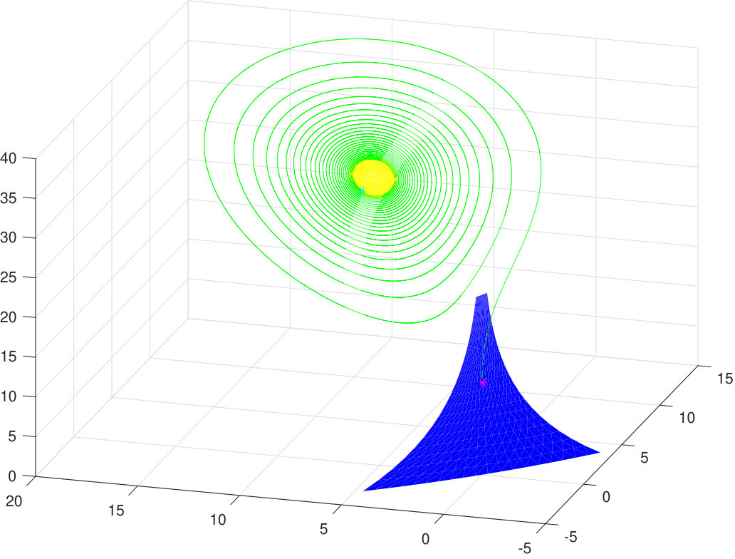 Figure 1
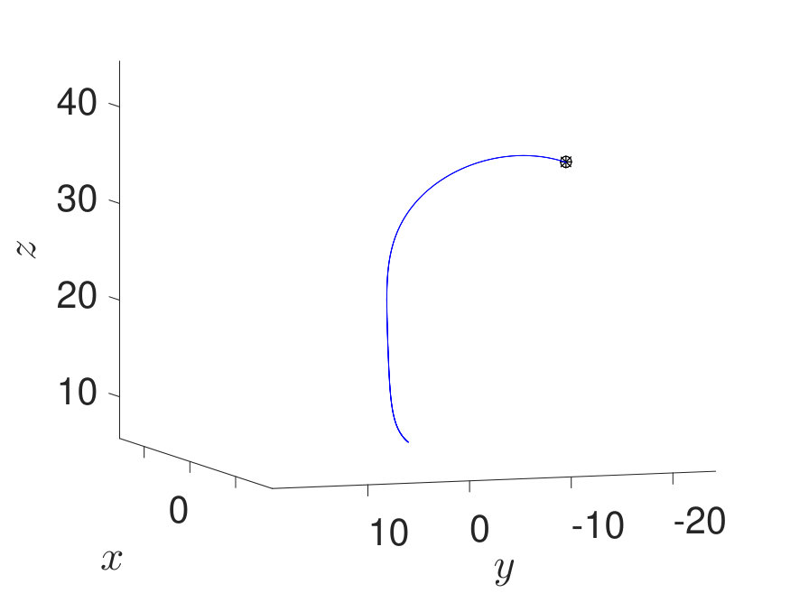 Figure 2
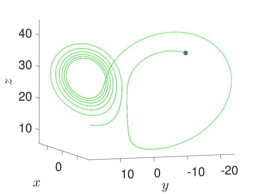 Figure 3
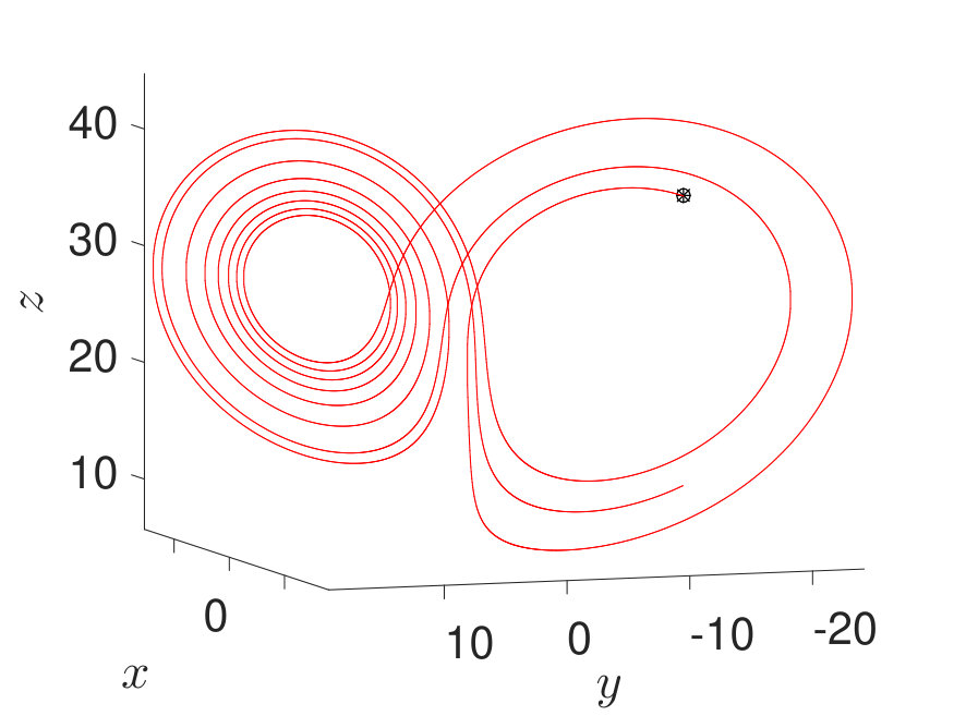 Figure 4
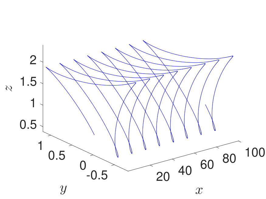 Figure 5
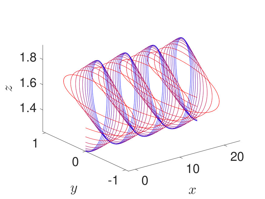 Figure 6
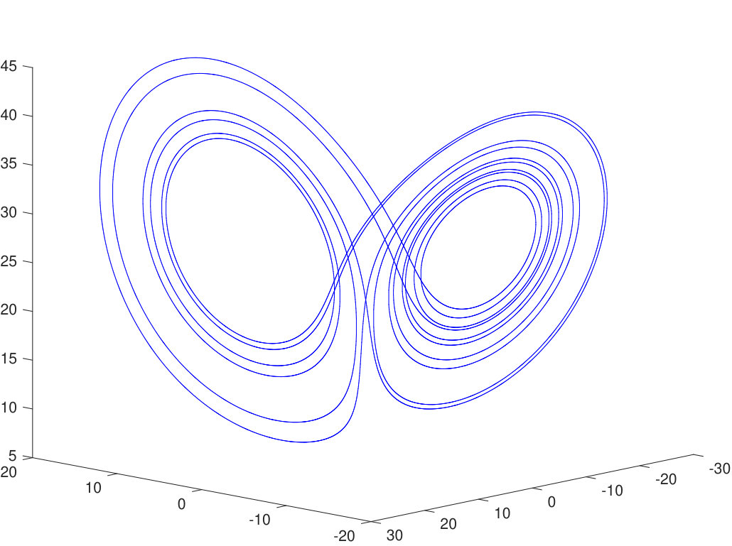 Figure 7
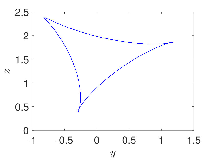 Figure 8
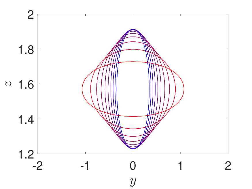 Figure 9
| 1 | 2333 | 13998 | 0.69 | |
| 2 | 1556 | 14004 | 0.64 | |
| 3 | 1167 | 14004 | 0.58 |
| 1 | 2333 | 13998 | 0.97 | |
| 2 | 1556 | 14004 | 5.6 | |
| 3 | 1167 | 14004 | 5.5 | |
| 4 | 933 | 13995 | 4.9 |
| 2 | 1556 | 14004 | 5.6 | |
| 3 | 1167 | 14004 | 8.1 | |
| 4 | 933 | 13995 | 8.1 | |
| 5 | 778 | 14004 | 8.0 | |
| 9 | 467 | 14010 | 7.9 | |
| 19 | 233 | 13980 | 6.9 |
| no proof | ||||
|---|---|---|---|---|
| no proof | ||||
Peer Reviews
No public reviews on file for this paper yet. If you reviewed it on a platform where reviews are public (OpenReview, ICLR, NeurIPS, ICML), you can paste yours below so the community can read it here.
Videos
No videos yet. Explain this paper in a talk, walkthrough, or lecture? Add one.
Taxonomy
TopicsNumerical Methods and Algorithms · Polynomial and algebraic computation · Advanced Differential Equations and Dynamical Systems
Polynomial interpolation and a priori bootstrap for computer-assisted proofs in nonlinear ODEs
Maxime Breden CMLA, ENS Cachan, CNRS, Université Paris-Saclay, 61 avenue du Président Wilson, 94230 Cachan, FranceDépartement de Mathématiques et de Statistique, Université Laval, 1045 avenue de la Médecine, Québec, QC, G1V 0A6, Canada.
Jean-Philippe Lessard22footnotemark: 2
Abstract
In this work, we introduce a method based on piecewise polynomial interpolation to enclose rigorously solutions of nonlinear ODEs. Using a technique which we call a priori bootstrap, we transform the problem of solving the ODE into one of looking for a fixed point of a high order smoothing Picard-like operator. We then develop a rigorous computational method based on a Newton-Kantorovich type argument (the radii polynomial approach) to prove existence of a fixed point of the Picard-like operator. We present all necessary estimates in full generality and for any nonlinearities. With our approach, we study two systems of nonlinear equations: the Lorenz system and the ABC flow. For the Lorenz system, we solve Cauchy problems and prove existence of periodic and connecting orbits at the classical parameters, and for ABC flows, we prove existence of ballistic spiral orbits.
Key words Computer-assisted proof Nonlinear ODEs Picard-like operator
Piecewise polynomial interpolation Newton-Kantorovich ABC flows
2010 AMS Subject Classification 65G20 65P99 65D30 37M99 37C27
1 Introduction
This paper introduces an approach based on polynomial interpolation to obtain mathematically rigorous results about existence of solutions of nonlinear ordinary differential equations (ODEs). Our motivation for the present work is threefold. First, we believe that polynomial interpolation techniques are versatile and can lead to efficient and general computational methods to approximate solutions of ODEs with complicated (non polynomial) nonlinearities. Second, while polynomial interpolation techniques have be used to produce computer-assisted proofs in ODEs, their applicability to produce proofs is sometimes limited by the formulation of the problem itself. More precisely, a standard way to prove (both theoretically and computationally) existence of solutions of systems of ODEs is to reformulate the problem into an integral equation (often in the form of a Picard operator) and then to apply the contraction mapping theorem to get existence. If one is interested to produce computer-assisted proofs using that approach, the analytic estimates required to perform the proofs depend on the amount of regularity gained by applying the integral operator. This observation motivated developing what we call the a priori bootstrap, which consists of reformulating the original ODE problem into one of looking for the fixed point of a higher order smoothing Picard-like operator. Third, we believe (and hope) that our proposed method can be adapted to study infinite dimensional continuous dynamical systems (e.g. partial differential equations and delay differential equations) for which spectral methods may sometimes be difficult to apply (for instance because of the shape of the spatial domains or because the differential operators are difficult to invert in a given spectral basis).
It is important to realize that computer-assisted arguments to study differential equations are by now standard, and that providing a complete overview of the literature would require a tremendous effort and is outside the scope of this paper. However, we encourage the reader to read the survey papers [1, 2, 3, 4, 5, 6], the books [7, 8] and to consult the webpage of the CAPD group [9] to get a flavour of the extraordinary recent advances made in the field.
More closely related to the present work are methods based on the contraction mapping theorem using the radii polynomial approach (first introduced in [10]), which has been developed in the last decade to study fixed points, periodic orbits, invariant manifolds and connecting orbits of ODEs, partial differential equations and delay differential equations (see for instance [11, 12, 13, 14, 15, 16]). The numerics and a posteriori analysis in those works mainly use spectral methods like Fourier and Chebyshev series, and Taylor methods. First order polynomial (piecewise linear) approximations were also used using the radii polynomial approach (see [17, 18, 19]), but more seldom, mainly because the numerical cost was higher and the accuracy was lower than for spectral methods. The computational cost of these low order methods is essentially due to the above mentioned low gain of regularity of the Picard operators chosen to perform the computer-assisted proofs.
In an attempt to address the low gain of regularity problem, we present here a new technique that we call a priori bootstrap which, when combined with the use of higher order interpolation, significantly improves the efficiency of computer-assisted proofs with polynomial interpolation methods. We stress that the limitations that affected the previous works using interpolation were not solely due to the use of first order methods, and that the a priori bootstrap is crucial (that is, just increasing the order of the interpolation does not significantly improve the results in those previous works). This point is illustrated in Section 6.
While we believe that one of the advantage of our proposed method is the versatility of the polynomial interpolations to tackle problems with complicated (non polynomial) nonlinearities, we hasten to mention the existence of previous powerful methods which have been developed in rigorous computing to study such problems. For instance, automatic differentiation (AD) techniques provide a beautiful and efficient means of computing solutions of nonlinear problems (e.g. see [7, 20, 21]) and are often combined with Taylor series expansions to prove existence of solutions of differential equations with non polynomial nonlinearities (e.g. see [1, 22, 23, 24, 25, 26, 27]). Also, in the recent work [28], the ideas of AD are combined with Fourier series to prove existence of periodic orbits in non polynomial vector fields. Independently of AD techniques, a method involving Chebyshev series to approximate the nonlinearities have been proposed recently in [29]. Finally, the fast Fourier transform (FFT) algorithm is used in [30] to control general nonlinearities in the context of computer-assisted proofs in KAM theory.
In this paper we consider a vector field (not necessarily polynomial) with , and we present a rigorous numerical procedure to study problems of the form
[TABLE]
We treat three special cases for , corresponding to an initial value problem, a problem of looking for periodic orbits and a problem of looking for connecting orbits. We also note that, as for the already existing spectral methods, the technique presented here extends easily to treat parameter dependent versions of (1) (e.g. using ideas from [31, 32, 33]). For the sake of simplicity, we expose all the general arguments for the initial value problem only, that is for
[TABLE]
given an integration time and an initial condition . We explain how (2) needs to be modified for different problems as we introduce them in Sections 6 and 7.
Our paper is organized as follows. In Section 2, we start by presenting our a priori bootstrap technique, together with a piecewise reformulation of the operator that we use throughout this work. We then recall in Section 3 some definitions and error estimates about polynomial interpolation, and explain how to combine them with our a priori bootstrap formulation to get computer-assisted proofs. The precise estimates needed for the proofs are then derived in Section 4, and their dependency with respect to the a priori bootstrap and to the parameters of the polynomial interpolation is commented in Section 5. This discussion is complemented by several examples in Section 6, where we apply our technique to validate solutions for the Lorenz system. Finally we give another example of application in Section 7, where we prove the existence of some specific orbits for ABC flows.
2 Reformulations of the Cauchy problem
2.1 A priori bootstrap
One of the usual strategies used to study (2), both theoretically and numerically, is to recast it as a fixed point problem, as in the following lemma.
Lemma 2.1**.**
Consider the standard Picard operator
[TABLE]
where
[TABLE]
Then is a fixed point of if and only if is a solution of (2).
In previous works using this reformulation, the limiting factor in the estimates needed to apply the contraction mapping theorem was a consequence of the fact that only gains one order of regularity, that is maps into . This fact will be made precise in Section 4 where we derive the estimates in question and in Section 5 where we discuss how those estimates affect the effectiveness of our technique.
To circumvent this limitation, we propose a different reformulation that we call a priori bootstrap. This approach provides operators which gain more regularity, and therefore lead to sharper analytic estimates. First we introduce some notations. The following definition allows concisely describing the higher order equations obtained by taking successive derivatives of (2).
Definition 2.2**.**
Consider the sequence of vector fields with ,
[TABLE]
Lemma 2.3**.**
For any , solves (2) if and only if solves the following Cauchy problem
[TABLE]
Proof.
The direct implication is trivial. To prove the converse application, we consider and show that is solve a linear ODE of order , with initial conditions for all , which implies that . ∎
Integrating the order Cauchy problem (4) times leads to a new fixed point operator which now maps into .
Lemma 2.4**.**
Let and consider the Picard-like operator
[TABLE]
where
[TABLE]
Then is a fixed point of if and only if is a solution of (4) (and thus of (2)).
Proof.
If is a fixed point of , an elementary computation yields that solves (4). Conversely, if solves (4) then Taylor’s formula with integral reminder shows that is a fixed point of . ∎
It is worth noting that, in the same framework of rigorous computation as the one used here, approximations using piecewise linear functions were used in [18] to prove existence of homoclinic orbits for the Gray-Scott equation. In that case the system of ODEs considered is of order , and therefore the equivalent integral operator is very similar to in (5) for . Similarly, piecewise linear functions were used in [19] to prove existence of connecting orbits in the Lorenz equations. In that case, the standard Picard operator (3) was used.
Now that we have an operator which provides a gain of several orders of regularity, it becomes interesting to consider polynomial interpolation of higher order, and again this will be detailed in Section 5 and applied in Section 6.
2.2 Piecewise reformulation of the Picard-like operator
We finish this section by a last equivalent formulation of the initial value problem (2), that will be the one used in the present paper to perform the computer-assisted proofs. Given , we introduce the mesh of
[TABLE]
where . Then we consider (respectively ) the space of piecewise continuous (respectively functions having possible discontinuities only on the mesh . More precisely, we use the following definition.
Definition 2.5**.**
For , we say that if and can be extended to a function on , for all .
We then introduce
[TABLE]
defined on the interval () by
[TABLE]
where denotes the left limit of at , and must be replaced by (this last convention will be used throughout the paper).
Remark 2.6**.**
We point out that our computer-assisted proof is based on the operator (defined in (6)), which differs slightly from the operator (defined in (5)), which was used in previous studies such as [17, 18, 19]. The only difference is that the integral in is in some sense reseted at each . We introduce this piecewise reformulation because it allows for sharper estimates (see Remark 4.7). **
We finally introduce as
[TABLE]
Lemma 2.7**.**
Let . Then if and only if solves (2).
Proof.
This result is similar to Lemma 2.4. The only additional property that we need to check is that, if satisfies , then cannot be discontinuous. Indeed, if then , and for all one has
[TABLE]
At this point, it might seems as if defining on brings unnecessary complications, and that we should simply define it on . While this is indeed a possibility, it will quickly become apparent that the present choice is more convenient, both for theoretical and numerical considerations (see Remark 3.4).
Finding a zero of is the formulation of our initial problem (2) that we are going to use in the rest of this paper.
3 General framework for the polynomial interpolation
3.1 Preliminaries
Given a mesh as defined in Section 2.2, we introduce the refined mesh where, for all we add points between and . More precisely we suppose that these points are the Chebyshev points (of the second kind) between and , that is we add the following points:
[TABLE]
where
[TABLE]
Notice that the above definition extends to and , and that corresponds to the mesh used in previous studies with first order interpolation (e.g. see [18, 19, 17]).
We then introduce the subspace of piecewise polynomial functions of degree on
[TABLE]
Next, we define the projection operator
[TABLE]
where is the function in that matches the values of on the mesh . Notice that can have discontinuities at the points , therefore the matching of and at those points must be understood as
[TABLE]
In the sequel we will need to control the error between a function and its interpolation . This is the content of the following propositions, where denotes the sup norm on .
Proposition 3.1**.**
For all ,
[TABLE]
where
[TABLE]
Proposition 3.2**.**
Fix such that . For all ,
[TABLE]
where
[TABLE]
* being the Lebesgue constant (see for instance [34]), and denoting the integer part of .*
Remark 3.3**.**
More information about the Lebesgue constant, and in particular sharp computable upper bounds for it, can be found in the Appendix, together with references and proofs of the two above propositions. **
3.2 Finite dimensional projection
To get an approximate zero of (and thus an approximate solution of (2)), we are going to look for a zero of . But first, we need a convenient way to represent the elements of . Here and in the sequel, we use the exponent (i) to denote the -th component of a vector in , but we will work with all the components at once as often as possible to avoid burdening the notations with this exponent (i). Let us introduce the set of indexes
[TABLE]
Perhaps the most natural way to characterize an element of is to give all the values for . However, we will also use another representation, more suited to numerical computations, which consists of decomposing on the Chebyshev basis. That is, we write
[TABLE]
where is the -th Chebyshev polynomial of the first kind. We can thus also describe uniquely any function belonging to by the family of Chebyshev coefficients .
Remark 3.4**.**
Let us mention how considering functions with possible discontinuities on the mesh points in comes in handy. By restricting ourselves to functions in , we would need additional constraints on the Chebyshev coefficients to impose the continuity at each of the mesh point () and keep track of them in all computations. Instead, the choice of working with allows avoiding these additional constraints. **
For we have
[TABLE]
We recall that all the values for uniquely characterize .
Using the isomorphisms and to identify and , we can in fact see as a function from to itself, that associates to the coefficients the values . Thus we can numerically find a zero of , which is going to be our approximate solution. We note that we use these identifications between and throughout the present work. Our objective is now to validate this numerical solution , that is to prove that within a given neighbourhood of lies a true zero of .
3.3 Back to a fixed point formulation
We consider the space and its decomposition , where
[TABLE]
We already have a projection onto
[TABLE]
and we also define its complementary
[TABLE]
We then define the norms
[TABLE]
On we consider the norm
[TABLE]
where is a positive parameter. Notice that for all , is a Banach space. For any , we denote by the closed neighbourhood of [math] defined as
[TABLE]
Suppose that we now have computed a numerical zero of . We define and consider an injective numerical inverse of . Finally, we introduce the Newton-like operator defined by
[TABLE]
Notice that the fixed points of are in one-to-one correspondence with the zeros of . We now give a finite set of sufficient conditions, that can be rigorously checked on a computer using interval arithmetic, to ensure that is a contraction on a given ball around . If those conditions are satisfied, the Banach fixed point theorem then yields the existence and local uniqueness of a zero of . This is the content of the following statement (based on [35], see also [10] for a detailed proof).
Theorem 3.5**.**
Let
[TABLE]
and
[TABLE]
Assume that we have bounds and satisfying
[TABLE]
[TABLE]
[TABLE]
and
[TABLE]
If there exist such that
[TABLE]
and
[TABLE]
then there exists a unique zero of within the set .
The quantities and given respectively in (15) and (16) are called the radii polynomials.
In the next section, we show how to obtain bounds and satisfying (11)-(14). Before doing so, let us make a quick remark about the different representations and norms we can use on .
Remark 3.6**.**
As explained in Section 3.2, in practice we will mostly work with represented by its Chebyshev coefficients as in (7). However, there are going to be instances where the values are needed, for instance to compute . We point out that numerically, passing from one representation to the other can be done easily by using the Fast Fourier Transform.
One other important point is that, at some point in the next section we are going to need upper bounds for . To get such a bound from our finite dimensional data, we have two options, namely
[TABLE]
or
[TABLE]
If is given, then (17) is usually better, whereas (18) is better if is any function in a given ball of . Notice that (17) simply follows from the fact that the Chebyshev polynomials satisfy for all and all . For more information about the bound (18), see the Appendix and the references therein. **
4 Formula for the bounds
In this section, we give formulas for , , and satisfying the assumptions (11)-(14) of Theorem 3.5. To make the exposition clearer, we focus strictly on the derivation of the different bounds in this section. In particular, the discussion about the impact of the level of an priori bootstrap (that is the value of ) and the order of polynomial approximation (that is the value of ) is done in Section 5.
4.1 The bounds
In this section we derive the bounds, which measure the defect associated with a numerical solution , that is how close is to [math]. We start by the finite dimensional part.
Proposition 4.1**.**
Let be defined as in (9) and consider
[TABLE]
where is here seen as the vector . Then (11) holds.
Proof.
Simply notice that . ∎
Remark 4.2**.**
The above bound is not completely satisfactory, in the sense that is not directly implementable. Indeed, to compute we need to evaluate (or at least to bound) the quantities . In particular (see (3.2)), we need to evaluate the integrals
[TABLE]
where
[TABLE]
If is a non polynomial vector field, we use a Taylor approximation of order of to get an approximate value of the integral by computing
[TABLE]
Notice that this quantity can be evaluated explicitly. The error made in this approximation is then controlled as follows
[TABLE]
Notice that this error term is effective, since can be bounded using interval arithmetic. Therefore, the quantity that we end up implementing is of the form
[TABLE]
where the vector contains the approximate integrals and the vector contains the errors bounds for these approximations. Here and in the sequel, absolute values applied to a matrix, like , must be understood component-wise. We point out that, in practice, if the mesh is refined enough, then is not going to be varying much on each subinterval , and thus we can get rather precise approximations even with a lower order for the Taylor expansion.
We mention that when the vector field is polynomial, has a finite Taylor expansion, therefore up the integrals can in fact be computed exactly (i.e. we can get ). **
We now turn our attention to the second part of the bound.
Proposition 4.3**.**
Let be defined as in (9) and consider
[TABLE]
Then (12) holds.
Proof.
We have . Since , we have that and Proposition 3.1 yields
[TABLE]
Remark 4.4**.**
As comment similar to the one of Remark 4.2 applies here. Indeed, the bound given in Proposition 4.3 is not directly implementable because of the term
[TABLE]
but we can again get an explicit bound for this quantity by using a low order Taylor approximation and interval arithmetic. In the particular case where the vector field is polynomial, an explicit bound can also be obtained via the Chebyshev coefficients of the polynomial , as in (17). **
4.2 The bounds
In this section we derive the bounds, which measure the contraction rate of on the ball of radius around . We begin with the finite dimensional part, that is the projection on . Let be defined as in (10). Then
[TABLE]
where and are defined as in Section 3.3. We are going to bound each term separately as
[TABLE]
4.2.1 The bound
The computation of the bounds estimating the first of the terms in the splitting (19) is rather straightforward and is simply a control on the precision of the numerical inverse.
Proposition 4.5**.**
Let , define the vector by for all and let
[TABLE]
Then,
[TABLE]
4.2.2 The bound
We now construct the bounds estimating the second term in the splitting (19).
Proposition 4.6**.**
Let , consider such that
[TABLE]
where is the vector of size whose components all are equal to . Let
[TABLE]
Then
[TABLE]
Proof.
By definition of and , we have that
[TABLE]
Therefore, we can rewrite
[TABLE]
and we only need to prove that
[TABLE]
Remembering (3.2) and using that , we estimate for all ,
[TABLE]
∎
Notice that Remark 4.4 also applies here.
Remark 4.7**.**
Had we used the operator (see (5)) instead of (see (6)), we would have gotten a bound like
[TABLE]
which is obviously worst because one has to consider the whole integral from [math] to instead of just from to . **
4.2.3 The bound
We finally construct the bounds estimating the last term in the splitting (19).
Proposition 4.8**.**
Let . consider such that
[TABLE]
Let
[TABLE]
Then
[TABLE]
Remark 4.9**.**
In the above proposition, must be understood as the evaluation of the -linear form at the vectors , that is
[TABLE]
Proof.
(of Proposition 4.8) We only have to prove that
[TABLE]
Using (18) we have that
[TABLE]
Then we estimate for all ,
[TABLE]
Notice that Remark 4.4 also applies here.
4.2.4 The bound
We are left with the remainder part of the bound, which we treat in this section.
Proposition 4.10**.**
Let and as in (10). Define for all
[TABLE]
where is one of the two constants given by Propositions 3.1 and 3.2, namely
[TABLE]
Then (14) holds.
Proof.
We need to estimate
[TABLE]
For any continuous function , one has
[TABLE]
thus we get, for all
[TABLE]
Notice that Remark 4.4 also applies here.
4.3 The radii polynomials and interval arithmetics
The following proposition sums up what has been proven up to now in this section, namely that we have derived bounds that satisfy the requirements (11) to (14) from Theorem 3.5.
Proposition 4.11**.**
Let and defined as in (9) and (10). Then, the bound defined in Proposition 4.1 satisfies (11) and the one from Proposition 4.3 satisfies (12). Also, consider the bounds defined in Propositions 4.5 to 4.8. Then
[TABLE]
satisfies (13) and finally the bound from Proposition 4.10 satisfies (14).
Notice that, the way these bounds are defined, they are polynomials in and , whose coefficients are all positive and can be computed explicitly with the help of the computer, since they depend on the numerical data of an approximate solution . Also, we make sure to control possible round-off errors by using interval arithmetic (in our case INTLAB [27]).
In practice, we first consider so that it satisfies the constraint (20) introduced in the next section. If there does not exist such positive , we increase and/or and/or and try again. Once is fixed, we try to find a positive such that the last conditions (15) and (16) of Theorem 3.5 hold. If there is no such positive , we increase and/or and/or and try again. If we finally find a positive satisfying (15) and (16), then we have proven that Theorem 3.5 applies, that is there exists a unique zero of in .
In Sections 6 and 7, we give several examples where the procedure described just above is successfully used to validate solutions of an initial value problem, as well as periodic solutions and heteroclinic orbits. But before doing so, we discuss in the next section the role of the parameters , and , and how they influence the bounds.
5 About the choice of the parameters
In this section, we explain how the parameters , and should be chosen, and in particular we highlight how the a priori bootstrap (that is taking ) helps improving the efficiency of the computer-assisted procedure we propose. The discussion will be rather informal, but we hope it helps the reader understand the results of the various comparisons presented in Section 6. Also, to make things slightly simpler we assume here that the grid is uniform, therefore in the estimates each instance of can be replaced by .
Our main constraint is that we want the method to be successful while minimizing the size of our numerical data, that is the dimension of our finite dimensional space , which is . Since is fixed by the dimension of the vector field , we want to minimize the product . As we see in the examples of Section 6, the usual limiting factor when trying to satisfy the radii polynomial inequalities (15) and (16) is to get the order one term (in ) to be negative. For the finite part (that is (15)), that means basically having that
[TABLE]
(see Proposition 4.6), and for the remainder part (that is (16)) we get a condition like
[TABLE]
where and are constants depending on the numerical solution and on the vector field , but not on the parameters , and that we can tune. This leads to
[TABLE]
We want to be able to chose a satisfying the above inequalities, and a necessary and sufficient condition for that is
[TABLE]
which we can rewrite
[TABLE]
Remember that we want (21) to be satisfied, while minimizing the product . When is fixed, and becomes large, notice that is decreasing like . However, satisfying (21) requires, roughly speaking, to decrease as much as possible. This suggests two things, which we confirm in our explicit examples of Section 6. First, that it is slightly better to increase than (because of the factor) and second, that if we take equal to 2 or more (that is if we use a priori bootstrap) then we can satisfy (21) while taking much smaller than if we had equal to 1.
Finally, we point out that taking seems optimal for the conditon (21) given by the order one term. Indeed, increasing from to increases the total number of coefficients, but brings no gain with respect to (21) since
[TABLE]
However, for the proof to succeed (that is for (15) and (16) to be satisfied) we also need small enough and bounds. Looking more precisely at , we see that it is of the form
[TABLE]
where depends on the numerical data and also on , but the dependency on is way less important than in the term, so we neglect it here. Looking back to the definition of in Proposition 3.1, we see that the term that we want to be small is of the form
[TABLE]
Therefore, if we really need to decrease the bound, increasing is drastically better than increasing . That is why, in practice we often take , even though would be enough to satisfy (21). Finally we point out that, if we are not simply focused on getting an existence result, but also care about having sharp error bound, then we should definitively take care of having small and bounds, which, as we will show in the next section, can be achieved by slightly increasing (that is taking ).
In the next section, we present several comparisons for different choices of parameters, that confirm the heuristic presented in this section.
6 Examples of applications for the Lorenz system
In this section, we consider the Lorenz system, that is
[TABLE]
with standard parameter values . Here, we first consider the initial value problem (2), and use those bounds to try and validate orbits of various length with different parameters, to highlight the significant improvement made possible by the a priori bootstrap technique (that is taking ). Then, we show that the a priori bootstrap also allows to validate more interesting solutions (from a dynamical point of view), namely periodic orbits and connecting orbits.
6.1 Comparisons for the initial value problem
The aim of this section is to showcase the improvements allowed by the use of a priori bootstrap, and to validate the heuristics made in Section 5. To do so, we fix an initial data (chosen close to the attractor of the Lorenz system)
[TABLE]
and do two kinds of comparisons. First, we try to validate the longest possible orbits for at various values of and . We recall that by validating, we mean getting the existence of a true solution near a numerical one, by checking that the hypotheses of Theorem 3.5 hold. To make the comparison fair, we fix the total number of coefficients used for the numerical approximation, that is the dimension of , given by . This quantity is usually the bottleneck of our approach, since we need to store and invert the matrix which is of size . Here, we take (or as close as possible to ). The computations were made on a laptop with 8GB of RAM, and of course could be taken larger on a computer with more memory.
The first set of results are given in Table 1 (we recall that we work with the Lorenz system, therefore ).
In all cases, the proof fails for longer time , because (21) is no longer satisfied. We see here that, as announced in Section 5, it is better to take as small as possible to get the longest possible orbit, but that increasing helps reducing the bound, and thus the validation radius . We see that simply increasing the order of the polynomial interpolation (given by ), allows to get better accuracy but does not really help to prove longer orbits. However, we are going to show on the next examples (see Table 2) that combining a priori bootstrap (that is taking ) with higher order polynomial interpolation does allow to get much longer orbits.
First, comparing the case when and , we see that using a priori bootstrap allows to get a slightly longer orbit, even for linear interpolation. Also, even for the longest possible orbit in that case (), we still have much room to satisfy (21) (the quantity given by (21) is ). However, we cannot get a longer orbit in that case even with , because the bound becomes too large. This can be dealt with by increasing , and we see that we can then get much longer orbits. To finish this set of comparisons, we show that doing one more iteration of the a priori bootstrap process (that is taking instead of ) still improves the results and allows to get longer orbits (see Table 3).
We sum up this set of comparisons by displaying the longest orbit obtained with , and (see Figure 1).
We then finish this section with another set of comparisons, where we now fix the length of the orbit, here , and instead look for the minimal total number of coefficients for which we can validate this orbit (for different values of ). The aim of this experiment is to show that using a priori bootstrap enables to validate solutions that one would not be able to validate without using it. Indeed, we are going to see that taking greater than one allows us to use way less coefficients to validate the solutions. Thus, if for a given solution, the proof without a priori bootstrap requires more coefficients than what our computer can handle, one can reduce this number by using a priori bootstrap and then possibly validate the orbit. For instance, still with the initial condition given by (22), we cannot validate the orbit of length without a priori bootstrap (that is with ), at least not with less that coefficients. However, the next table of results shows that we can validate it with , and also using even less coefficients with .
6.2 Validation of a periodic orbit.
To study periodic orbits, instead of an initial value problem, the system (1) has to be slightly modified into a boundary value problem
[TABLE]
where is now an unknown of the problem, and where . The last equation is sometimes called Poincaré phase condition and is here to isolate to periodic orbit.
As for the initial value problem, we can then consider an equivalent integral formulation (possibly with a priori bootstrap) and define an equivalent fixed point operator very similar to the one introduced in Section 3. The additional phase condition and the fact that is now a variable only require minor modifications of and of the bounds derived in Section 4 (see for intance [12]).
Using a priori bootsrtap, we are able to validate fairly complicated periodic orbits (see Figure 2).
6.3 Validation of a connecting orbit
In this section, we present a computer-assisted proof of existence of a connecting orbit in the Lorenz system for the standard parameter values . It is well know that at these parameter values, the Lorenz system admits a transverse connecting orbit between and the origin.
While computer-assisted proofs of connecting orbits were already investigated several times using topological and analytical approaches (see [18, 19, 25, 36, 37, 38, 39, 40, 41, 42, 43, 44, 45, 46, 47]), a paper of particular relevance to the present work is [19], where a particular case of our method is developed, with only linear interpolation and no a priori bootstrap (that is and ). While the authors in [19] were able to validate several connecting orbits for the Lorenz system, they could not validate the aforementioned connecting orbit for the standard parameter values. In fact, one of the main motivations for the present work was to improve the setting of [19] to be able to validate more complicated orbits.
As we showcased in Section 6.1, using a priori bootstrap enables us to validate significantly more complicated orbits for the initial value problem, and this is also true for connecting orbits. Indeed we are able to validate the standard connecting orbit for the Lorenz system, with parameter values . Before exposing the results, we briefly describe how to modify (2) to be able to handle connecting orbits.
Compared to an initial value problem on a given time interval, or to a periodic orbit, connecting orbits present an aditionnal difficulty which is that they are defined on an infinite time interval (from to ). To circumvent this difficulty and get back to a time interval of finite length, which is more suited to numerical computations (and to computer-assisted proofs), we are going to use local stable and unstable manifolds of the fixed points. By a computer-assisted method very similar to the one presented here, we first compute and validate local parameterization of the unstable manifold at and of the stable manifold at the origin. Since the main object of this work is not the rigorous computations of those manifolds, we simply assume that they are given (with validation radius) and do not give more details here. The interested reader can find more information about the computations and validations of these parameterizations in [13, 48] and the references therein, and also more detailed examples of their usage to get connecting orbits in [18, 19, 11, 12].
We denote by a local parameterization of the stable manifold of the origin, and by a local parameterization of the unstable manifold of a local parameterization of the stable manifold of . We point out that both manifolds are two-dimensional. We then want to solve
[TABLE]
where and each is a one dimensional parameter, the parameter in the other dimension being fixed to isolate the solution. Notice that is now an unknown of the system. As for the initial value problem, we can then consider an equivalent integral formulation (possibly with a priori bootstrap) and define an equivalent fixed point operator very similar to the one introduced in Section 3. The additional equation and the fact that we have three additional variables , and only requires minor modifications of and of the bounds derived in Section 4 (see for intance [12, 19]).
Using , and (that is a total number of 13803 coefficients) we are then able to rigorously compute a solution of (24) (see Figure 3).
7 Examples of applications for ABC flows
In this section, we apply our method to the non polynomial vector field
[TABLE]
The map is usually referred to as the Arnold-Beltrami-Childress (ABC) vector field, and gives a prime example of complex steady incompressible periodic flows in 3D (see [49, 50, 51] and the references therein).
The main point of this section is to briefly illustrate the applicability of our technique to non polynomial vector fields. We plan on studying more thoroughly ABC flows with the help of our a posteriori validation method in a future work. Recently, the existence of orbits, that are periodic up to a shift of in one coordinates, have been proven in the cases and [52, 53]. Applying the method developed in this paper, we were able to complete these results by proving the following statements.
Theorem 7.1**.**
For all , with , there exists (see Table 5) and a solution of the ABC flow such that
[TABLE]
Proof.
The proof is done by running script_proofs_A11.m (available at [56]), which for each computes an approximate solution, then computes bounds satisfying (11)-(14) as described in Section 4, and finally finds positive and such that (15)-(16) holds. ∎
Theorem 7.2**.**
For all , there exists and a solution of the ABC flow such that
[TABLE]
and .
Proof.
The proof is done by running script_proofs_111.m (available at [56]), which computes an approximate solution, then computes bounds satisfying (11)-(14) as described in Section 4, and finally finds positive and such that (15)-(16) holds. ∎
The solutions given by Theorem 7.1 are represented in Figure 4, and the solution given by Theorem 7.2 is represented in Figure 5.
Appendix
For the sake of completeness, we give here some properties of the Lebesgue constant , as well as proofs of Proposition 3.1 and Proposition 3.2. We will assume here that is defined and smooth on . The corresponding estimates on can the easily be deduced by rescaling.
We recall that is defined as the norm of the interpolation operator mapping to itself, and associating a continuous function to its interpolation polynomial of order . Of course this operator (and its norm) depend on the interpolation points, which in this work are the Chebyshev interpolation points of the second kind
[TABLE]
Introducing the basis consisting of the Lagrange functions
[TABLE]
we have that the Lagrange interpolation polynomial of order is given by
[TABLE]
One can then show (see for instance [34]), that
[TABLE]
and therefore we get
[TABLE]
which is exactly (18).
Since we used several times (18) and Proposition 3.2 in Section 4, the bounds that we obtained there depend on the Lebesgue constant . Therefore we need computable (and as sharp as possible) upper bounds for . One possibility is to use the well known bound (again see for instance [34])
[TABLE]
However, we can do better, at least when is odd. In that case, it has been shown (see [54]) that
[TABLE]
and this formula can be evaluated rigorously using interval arithmetic. Unfortunately, there is no such formula for even. For small values ( and ) we computed by hand using (26), and for we used (27) (it is also know that , therefore (27) is sharp for large ).
We now turn our attention to the interpolation estimates of Section 3. We point out that the analogue of Proposition 3.1 for the Chebyshev interpolation points of the first kind is very standard, and can be found in many textbooks. However, the case of the Chebyshev interpolation points of the second kind is seldom discussed, therefore we include a proof here for the sake of completeness (which is nothing but a slight adaptation of the standard proof).
Proof of Proposition 3.1. We consider the polynomial and use the standard interpolation error estimate for a function (see for instance [55]),
[TABLE]
To prove Proposition 3.1, we only have to show that (the remaining factor coming from the rescaling). Introducing, for , the -th Chebyshev polynomial of the second kind , defined by
[TABLE]
we have that
[TABLE]
Indeed, the right hand side of (28) is a unitary polynomial of degree , that has the same zeros as . We can then rewrite
[TABLE]
and we end up with
[TABLE]
so Proposition 3.1 is proven. ∎
Proof of Proposition 3.2. The first part of the bound, namely
[TABLE]
comes from a combination of the Lebesgue constant and Jackson’s Theorem, and can be found in [55]. However, it does not give a very sharp interpolation error estimate for small values of and , therefore we derive here the second part of the bound, namely
[TABLE]
that can be used in those cases.
Letting (with ) in (25) leads to
[TABLE]
We now fix a function . Using (29) with (that is ), we get
[TABLE]
Using Taylor’s formula, we then get
[TABLE]
for some in . Then, expanding the terms and using again (29), we get that
[TABLE]
and thus
[TABLE]
Letting
[TABLE]
we can easily observe that , and therefore
[TABLE]
According to [34], in case the points are the Chebyshev interpolation points of the second kind, we have
[TABLE]
Remembering that , we get
[TABLE]
The function
[TABLE]
is even and increasing on , therefore its maximum is reached at and we get
[TABLE]
Then, we compute
[TABLE]
We end up with
[TABLE]
and Proposition 3.2 is proven (the lacking factor coming from the time rescaling). ∎
The reference list from the paper itself. Each links out to its DOI / PubMed record.
- 1[1] Kyoko Makino and Martin Berz. Taylor models and other validated functional inclusion methods. Int. J. Pure Appl. Math. , 4(4):379–456, 2003.
- 2[2] Hans Koch, Alain Schenkel, and Peter Wittwer. Computer-assisted proofs in analysis and programming in logic: a case study. SIAM Rev. , 38(4):565–604, 1996.
- 3[3] Siegfried M. Rump. Verification methods: rigorous results using floating-point arithmetic. Acta Numer. , 19:287–449, 2010.
- 4[4] Jason D. Mireles James and Konstantin Mischaikow. Computational proofs in dynamics. In Bjorn Engquist, editor, Encyclopedia of Applied and Computational Mathematics , pages 288–295. Springer, 2015.
- 5[5] M. T. Nakao. Numerical verification methods for solutions of ordinary and partial differential equations. Numer. Funct. Anal. Optim. , 22(3-4):321–356, 2001.
- 6[6] Jan Bouwe van den Berg and Jean-Philippe Lessard. Rigorous numerics in dynamics. Notices of the American Mathematical Society , 62(9):1057–1061, 2015.
- 7[7] Warwick Tucker. Validated numerics . Princeton University Press, Princeton, NJ, 2011. A short introduction to rigorous computations.
- 8[8] Alex Haro, Marta Canadell, Jordi-Lluis Figueras, Alejandro Luque, and Josep-Maria Mondelo. The parameterization method for invariant manifolds: From rigorous results to effective computations , volume 195 of Applied Mathematical Sciences . Springer, 2016.