Large-scale distributed Kalman filtering via an optimization approach
Mathias Hudoba de Badyn, Mehran Mesbahi

TL;DR
This paper introduces a novel distributed Kalman filtering method that employs an optimization approach, specifically gradient descent, to efficiently estimate the error covariance matrix in large-scale sensor networks.
Contribution
It extends existing distributed Kalman filtering techniques by integrating an optimization-based update for the error covariance, reducing computational complexity in high-dimensional systems.
Findings
The proposed method effectively reduces computational costs.
The filter maintains accuracy comparable to traditional approaches.
Applications demonstrate improved scalability in sensor networks.
Abstract
Large-scale distributed systems such as sensor networks, often need to achieve filtering and consensus on an estimated parameter from high-dimensional measurements. Running a Kalman filter on every node in such a network is computationally intensive; in particular the matrix inversion in the Kalman gain update step is expensive. In this paper, we extend previous results in distributed Kalman filtering and large-scale machine learning to propose a gradient descent step for updating an estimate of the error covariance matrix; this is then embedded and analyzed in the context of distributed Kalman filtering. We provide properties of the resulting filters, in addition to a number of applications throughout the paper.
Click any figure to enlarge with its caption.
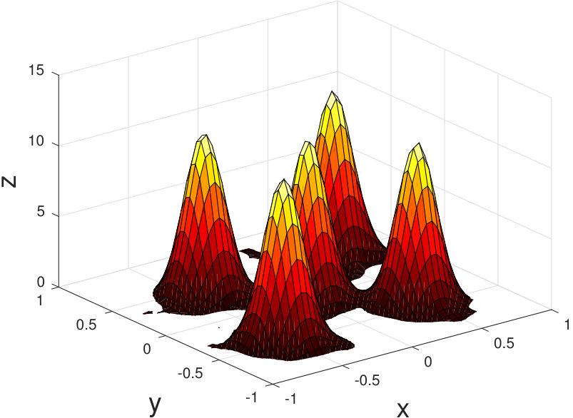 Figure 1
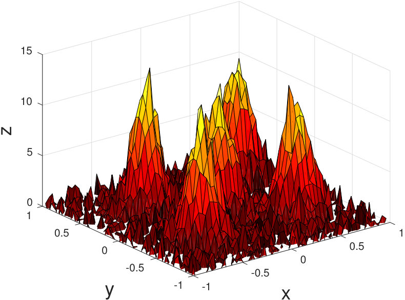 Figure 2
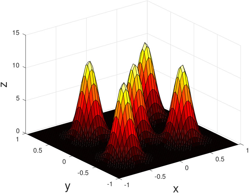 Figure 3
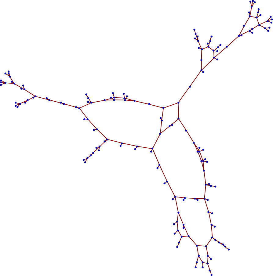 Figure 4
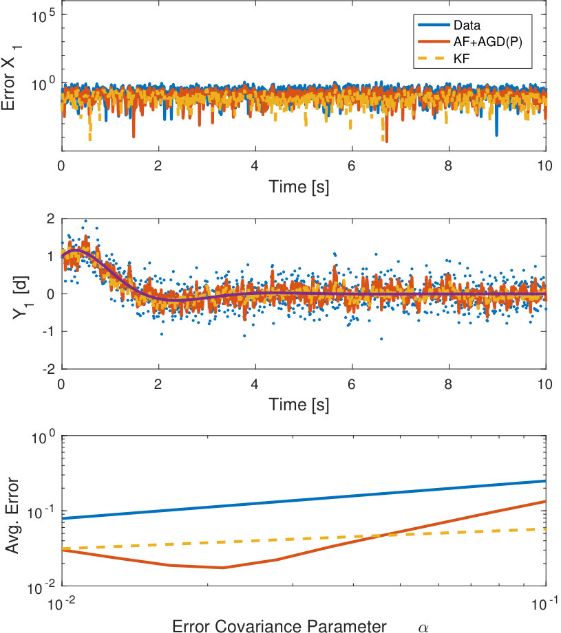 Figure 5
Peer Reviews
No public reviews on file for this paper yet. If you reviewed it on a platform where reviews are public (OpenReview, ICLR, NeurIPS, ICML), you can paste yours below so the community can read it here.
Videos
No videos yet. Explain this paper in a talk, walkthrough, or lecture? Add one.
Large-Scale Distributed Kalman Filtering via an Optimization Approach
Mathias Hudoba de Badyn∗ Mehran Mesbahi∗
∗William E. Boeing Department of Aeronautics and Astronautics, University of Washington, Seattle, WA 98195 USA
(e-mails: {hudomath,mesbahi}@uw.edu).
Abstract
Large-scale distributed systems such as sensor networks, often need to achieve filtering and consensus on an estimated parameter from high-dimensional measurements. Running a Kalman filter on every node in such a network is computationally intensive; in particular the matrix inversion in the Kalman gain update step is expensive. In this paper, we extend previous results in distributed Kalman filtering and large-scale machine learning to propose a gradient descent step for updating an estimate of the error covariance matrix; this is then embedded and analyzed in the context of distributed Kalman filtering. We provide properties of the resulting filters, in addition to a number of applications throughout the paper.
keywords:
Machine learning, fast Kalman algorithms, state estimation, gradient methods
††thanks: This research was supported by the U.S. Army Research Laboratory and the U.S. Army Research Office under contract number W911NF-13-1-0340 and AFOSR grant FA9550-16-1-0022.
1 Introduction
The Kalman filter is an algorithm that uses the known dynamics of a system to remove noise from measurements of that system. When considering large-scale dynamical systems, implementation of the standard or extended Kalman filters can be computationally difficult. In such cases, the Kalman filter requires the inversion of very large matrices at each timestep. This may cause the Kalman filter to run slower than the dynamical process it is trying to measure, or to severely reduce the temporal resolution of the measurements.
There are many systems for which measurements are taken by a network of sensors and are of high dimension; examples of such systems can be found in Khan and Moura (2008) and Kutz (2013). Previous methods for circumventing this problem include decomposing the dynamical system being measured into several subsystems and distributing the subsystems over the sensor network as in Khan and Moura (2008), or using Monte-Carlo methods for estimating the error covariance, such as in Furrer and Bengtsson (2007).
Previously, Sutton (1992) proposed to modify the Kalman filter error covariance update with a gradient descent method for the purpose of mimimizing memory consumption, albeit for a specific instantiation of a SISO linear system. In this paper, we extend the gradient descent algorithm for estimating the Kalman filter error covariance to the general MIMO linear system as a proposed solution to the problem of running a Kalman filter on a high-dimensional system. We improve the gradient descent using Nesterov acceleration and adaptive learning rate methods. Lastly, we apply the methods above to distributed Kalman filtering on a sensor network.
Distributed Kalman filtering seeks to estimate the state of a system by distributing the tasks of measuring the system and subsequently filtering the data to many agents, who then collectively assemble the state estimate. Such algorithms utilizing consensus to provide a global estimate were presented by Olfati-Saber (2005) and Olfati-Saber (2007), and later extended by Carli et al. (2008). Performance of distributed Kalman filters using graph-theoretic quantities were studied by Spanos et al. (2005).
The organization of the paper is as follows. In §2, we outline the mathematical notation and conventions we use. We discuss the gradient descent algorithm, Nesterov acceleration and adaptive learning rate methods in §3, and the distributed version of these algorithms with a relevant example in §4. The paper is summarized in §5.
2 MATHEMATICAL PRELIMINARIES
In this section, we lay out the mathematical notation used in this paper, and summarize the essential background on Kalman filtering.
Consider the noisy discrete-time controlled linear system
[TABLE]
where denotes the state vector, denotes the control vector, is the output vector or measurement, and are Gaussian white noise vectors of appropriate dimensions with covariances and respectively. The subscript refers to the timestep. The random vectors and represent system disturbances and sensor noise respectively, and the matrix describes how the disturbance propagates into the system. Since most matrix quantities will have a subscript denoting the timestep, we will refer to the th entry of a matrix with bracketed superscripts: . Similarly, the th entry of a vector is denoted , the th column of a matrix is denoted and the th row is denoted .
A network is represented by a graph where is a set of nodes representing agents in the network, and is the set of edges representing the connections between agents and . The neighbourhood set of node is the set of indices such that is an edge. We assume for simplicity that the graph is undirected, meaning that and represent the same edge.
The purpose of Kalman filtering is to provide an accurate estimate of the state using the measurement and the known information about the system and noise. The standard discrete-time linear Kalman filter yields the estimate and is given by
[TABLE]
where is the Kalman gain and is the error covariance matrix. The problem for high-dimensional systems is the inverse when computing . In this paper, we assume that the sensor noise is uncorrelated, and so is a diagonal positive-definite matrix. This leaves the term ; if this term is diagonal, then the matrix inverse becomes a series of scalar divisions. We propose to replace with a diagonal estimate , and one can also assume that is a matrix that measures individual states of the system without redundancy. Therefore, a system with outputs will have a measurement matrix of the form . This assumption is common for networked systems where one measures the state of individual nodes of the network, see for example Chapman and Mesbahi (2015). In the next few sections, we will formalize these assertions in the context of our algorithm.
3 GENERAL KALMAN FILTERING
In this section, we extend the gradient descent estimate for the error covariance proposed by Sutton (1992). In §3.1, we discuss the linear Kalman filter, and then extend the error covariance estimate to an accelerated gradient descent in §3.2. The accelerated gradient descent benefits from a clever adaptive learning rate, which is discussed in §3.3. The final algorithm combining all these methods is summarized in Algorithm 2.
3.1 Gradient Descent for the Error Covariance Update: Linear Case
Gradient descent is an iterative algorithm that seeks to find the local minimum of a function by stepping in the direction of the largest gradient:
[TABLE]
where is the learning rate. For the Kalman filter, we seek to find a diagonal matrix estimate of . We do this by assuming is of the form , where is a parameter undergoing gradient descent attempting to minimize the norm of the error :
[TABLE]
Computing the gradient of as outlined in Appendix A yields the following gradient descent equations for :
[TABLE]
[TABLE]
The form of guarantees that it remains positive-definite, which is required to preserve convergence of the Kalman filter.
3.2 Nesterov-Accelerated Methods
Nexterov acceleration is a method used to increase the convergence rate of gradient descent [Nesterov (1983)]. Although Nesterov-accelerated gradient descent converges in fewer timesteps, it does so by sacrificing monotonicity: the gradient descent trajectory will tend to oscillate as it converges towards the estimate.
In order to implement Nesterov acceleration, one must see that the quantity is a function of , which in turn is a function of :
[TABLE]
Hence, we can get the form of the Nesterov-accelerated gradient descent by introducing the quantity :
[TABLE]
where is given by
[TABLE]
Therefore, the Nesterov-accelerated estimate replaces the covariance update with the following equations:
[TABLE]
[TABLE]
where is as in Equation (1), but using this new expression for in Equation (2).
3.3 Adaptive Learning Rate Methods
Using a constant learning rate can lead to suboptimal performance, and therefore it is prudent to adapt on-the-fly as the gradient descent is run. A well-known method for adapting the learning rate is given by Barzilai and Borwein Barzilai and Borwein (1988). Suppose we have the gradient descent with learning rate :
[TABLE]
Let and let . Then, the Barzilai and Borwein method selects the learning rate parameter using a secant line approximation:
[TABLE]
For accelerated gradient descent, the updated learning rate is given by
[TABLE]
Combining the accelerated gradient descent estimate of the error covariance with the adaptive learning rate yields the final algorithm as outlined in Algorithm 1.
3.4 Filter Properties
In the standard Kalman filter, is computed from an algebraic Ricatti equation. In order for this equation to have a positive-definite solution, a requirement for stable error dynamics, one must assume that is stabilizable and is detectable (see Dorato et al. (1994)). Therefore, since our estimate of is positive definite by construction and not computed by an algebraic Ricatti equation, we do not need to have these assumptions. The next theorem shows that all one needs for stability of the error dynamics is for the system matrix to be stable.
Theorem 1
Suppose is an asymptotically stable matrix, and so the eigenvalues of satisfy . Then, the error dynamics
[TABLE]
are stable, where is the estimate computed according to Algorithm 1.
{pf}
We can write the error dynamics as
[TABLE]
where is given by
[TABLE]
Hence, it suffices to show that has eigenvalues in the unit disc. We can write as
[TABLE]
where . By the form of and , if the system has outputs, then is a diagonal matrix with the form
[TABLE]
It is clear that since is a positive definite diagonal matrix. Therefore, , and so it follows that
[TABLE]
and so by the asymptotic stability of , the asymptotic stability of follows.
3.5 Example
Here, we show a simple numerical implementation of Algorithm 1 to see how the algorithm performs compared to the standard Kalman filter for different strengths of noise. Consider the linear system with matrices
[TABLE]
propagating with process noise of covariance and measurement noise of covariance for various values of . The first and second plots of Figure 1 show the error and first state of the system for for the raw measurement data, and the filtered data using the accelerated gradient descent and the standard Kalman filter. The third plot shows the average steady state error computed on the time interval for various values of indicating the covariance of the measurement error. Figure 1 shows that the filter in Algorithm 1 achieves similar performance as the standard Kalman filter.
4 DISTRIBUTED KALMAN FILTERING
Olfati-Saber (2007) describes several methods of Kalman filtering using a network of sensors, with each th sensor using a unique sensor model , to arrive at a global measurement of a system. The context of their system model is on a graph , which is an abstract representation of the connection structure of sensors, which are represented by nodes. An edge in the graph denotes a communication link between sensors by which they can exchange information about their current state estimate. One such information exchange algorithm is called consensus, where each node in the graph changes its estimated value by continuously averaging with the estimates of its neighbours:
[TABLE]
One particular algorithm in Olfati-Saber (2007) utilizes a Kalman-consensus filter in which every node of the network computes an estimate of the state of the system and then performs consensus with its neighbours on this estimate. This allows sensors that only see a portion of the system to collect a global state estimate over time.
For high-dimensional systems, implementing this filter is problematic again because each sensor has to invert a large matrix at each timestep in order to compute the Kalman filter gain. In Algorithm 2, we summarize the Kalman-consensus filter, where every node performs an accelerated gradient descent with adaptive learning rate, and shares its estimate with its neighbours. In the following section, we provide an example of such a high-dimensional system.
4.1 Example
Consider a physical phenomenon, such as weather, propagating on a planar surface according to the partial differential equation
[TABLE]
As studied in Khan and Moura (2008), and Kutz (2013), by discretizing the surface into an equally-spaced grid in the and directions and the temporal dimension, thus obtaining a grid of values , one can construct the linear system representation
[TABLE]
where is a tridiagonal matrix with ’s on the sub and superdiagonal, and ’s on the diagonal. The discrete-time state matrix can be found using a matrix exponential, or a finite-order Taylor expansion. Periodic boundary conditions may be added by setting . Suppose that this phenomenon is being measured according to this discretization. We use a sensor model such that each node collects data from an square portion of the grid so that each individual grid point is measured by at least one sensor. The sensor network by the graph in Figure 2 is used, with for a grid, and the sensor noise is given unit covariance. Five 2D Gaussian functions are used to set the initial conditions for the simulation, which was run over a time interval of 10 seconds. The true state of the system at 1.2s is shown in Figure 3, and an aggregate measurement of the entire system is shown in Figure 4. An estimate from a single sensor at this timestep is shown in Figure 5, and one can see that there is a substantial reduction of noise.
5 Conclusion
In this paper, we extended the results of Sutton (1992) to produce a gradient descent estimate of the error covariance in a standard state estimation algorithm for linear systems. This gradient descent method was improved with Nesterov acceleration and an adaptive learning rate algorithm.
Finally, the algorithm was extended to improve the Kalman-consensus filter on a sensor network observing a distributed high-dimensional process. The diagonal estimate of removes the necessity of computing a large matrix inverse at each timestep at each sensor node, and allows for a computationally cheaper and therefore faster state estimation of the system over the entire network. The modified Kalman-consensus filter was implemented on a simple 2D diffusion model with 2500 grid points corresponding to the states of the system, and the algorithm was shown to remove a substantial amount of noise from the measurements, and to propagate the state estimate quickly across the sensor network.
Appendix A Gradient Descent for Kalman Filter Covariance Update
Sutton’s Gradient Descent for updating the error covariance matrix approximation uses gradient descent on :
[TABLE]
where is the error: To derive the exact form of the gradient descent on , consider the following terms:
[TABLE]
Next, we have
[TABLE]
We assume that for ,
[TABLE]
Next, define the following two quantities:
[TABLE]
Next, we compute the following derivatives:
[TABLE]
Now, we can write the gradient descent on :
[TABLE]
All that remains is to find an approximation to . We denote this approximation with :
[TABLE]
This yields the final gradient descent update:
[TABLE]
In conclusion, the Kalman filter with gradient descent error covariance update is given by the equations
[TABLE]
The reference list from the paper itself. Each links out to its DOI / PubMed record.
- 1Barzilai and Borwein (1988) Barzilai, J. and Borwein, J.M. (1988). Two-point step size gradient methods.
- 2Carli et al. (2008) Carli, R., Chiuso, A., Schenato, L., and Zampieri, S. (2008). Distributed Kalman filtering based on consensus strategies. IEEE Journal on Selected Areas in Communications , 26(4), 622–633.
- 3Chapman and Mesbahi (2015) Chapman, A. and Mesbahi, M. (2015). State controllability, output controllability and stabilizability of networks : A symmetry perspective. In Proc. 54th IEEE Conference on Decision and Control , 4776–4781. Osaka, Japan.
- 4Dorato et al. (1994) Dorato, P., Cerone, V., and Abdallah, C. (1994). Linear-Quadratic Control: An Introduction . Simon & Schuster.
- 5Furrer and Bengtsson (2007) Furrer, R. and Bengtsson, T. (2007). Estimation of high-dimensional prior and posterior covariance matrices in Kalman filter variants. Journal of Multivariate Analysis , 98(2), 227–255.
- 6Khan and Moura (2008) Khan, U.A. and Moura, J.M.F. (2008). Distributing the Kalman filter for large-scale systems. IEEE Transactions on Signal Processing , 56(10), 4919–4935.
- 7Kutz (2013) Kutz, J.N. (2013). Data-driven modeling & scientific computation: Methods for complex systems & big data . Oxford University Press.
- 8Nesterov (1983) Nesterov, Y. (1983). A method of solving a convex programming problem with convergence rate O (1/k^2). In Soviet Mathematics Doklady , volume 27, 372–376.