TL;DR
Mo3 is a flexible, accurate, and intuitive modular mobility model for 5G networks that captures complex mobility correlations without high complexity, improving upon existing models like RPGM.
Contribution
The paper introduces Mo3, a novel rule-based mobility model that combines accuracy and flexibility with simplicity, suitable for 5G and beyond networks.
Findings
Mo3 matches RPGM in topological properties.
Mo3 preserves spatial correlation better than RPGM.
Mo3 is simpler to set up and tune.
Abstract
Mobility modeling in 5G and beyond 5G must address typical features such as time-varying correlation between mobility patterns of different nodes, and their variation ranging from macro-mobility (kilometer range) to micro-mobility (sub-meter range). Current models have strong limitations in doing so: the widely used reference-based models, such as the Reference Point Group Mobility (RPGM), lack flexibility and accuracy, while the more sophisticated rule-based (i.e. behavioral) models are complex to set-up and tune. This paper introduces a new rule-based Modular Mobility Model, named Mo3, that provides accuracy and flexibility on par with behavioral models, while preserving the intuitiveness of the reference-based approach, and is based on five rules: 1) Individual Mobility, 2) Correlated Mobility, 3) Collision Avoidance, 4) Obstacle Avoidance and 5) Upper Bounds Enforcement. Mo3 avoids…
Click any figure to enlarge with its caption.
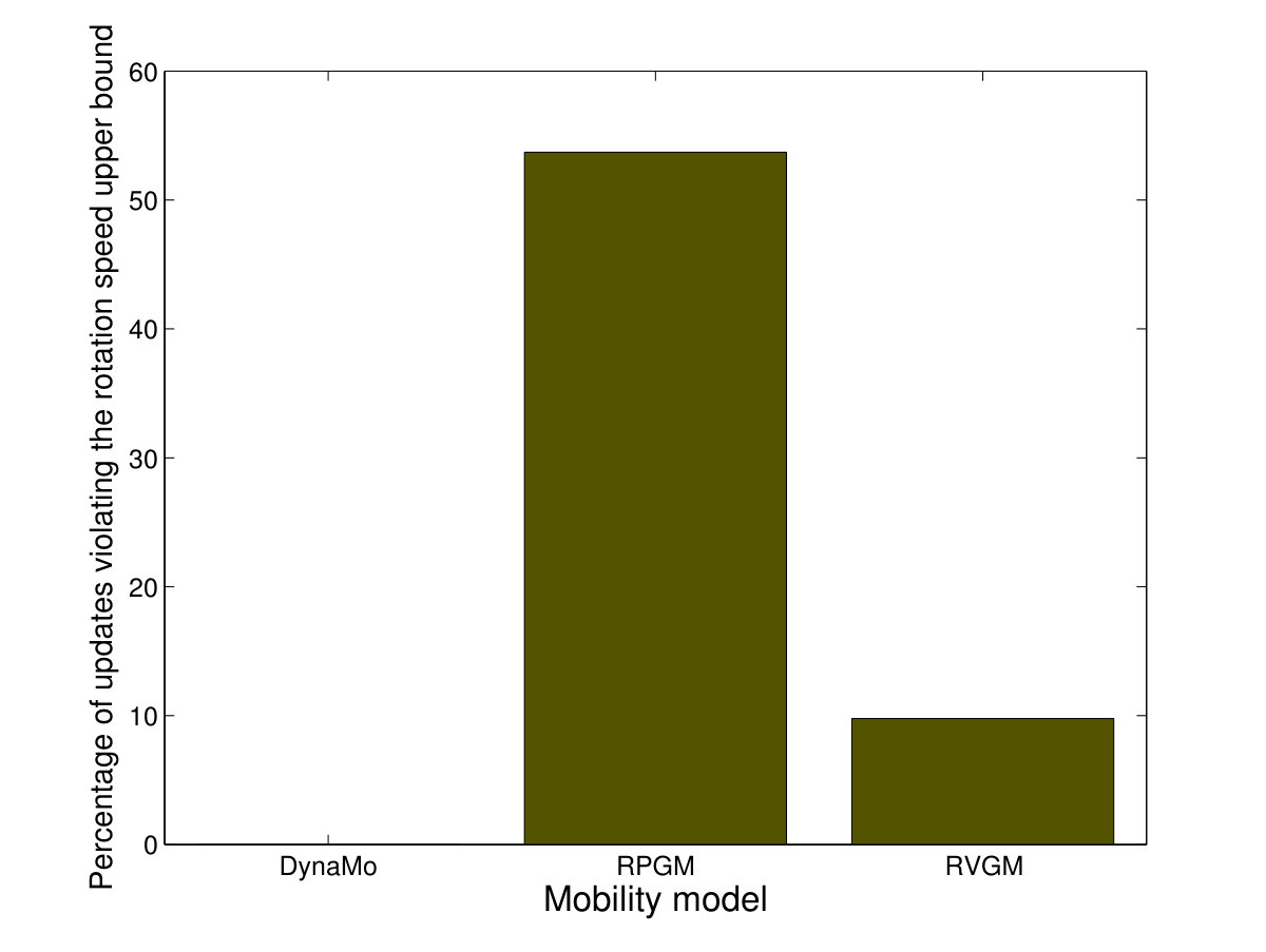 Figure 1
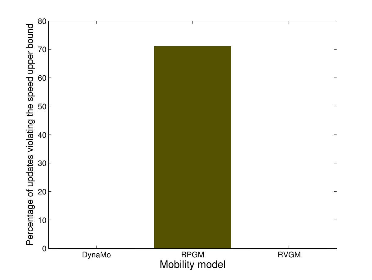 Figure 2
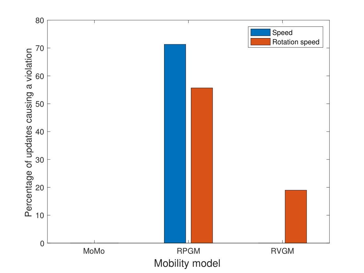 Figure 3
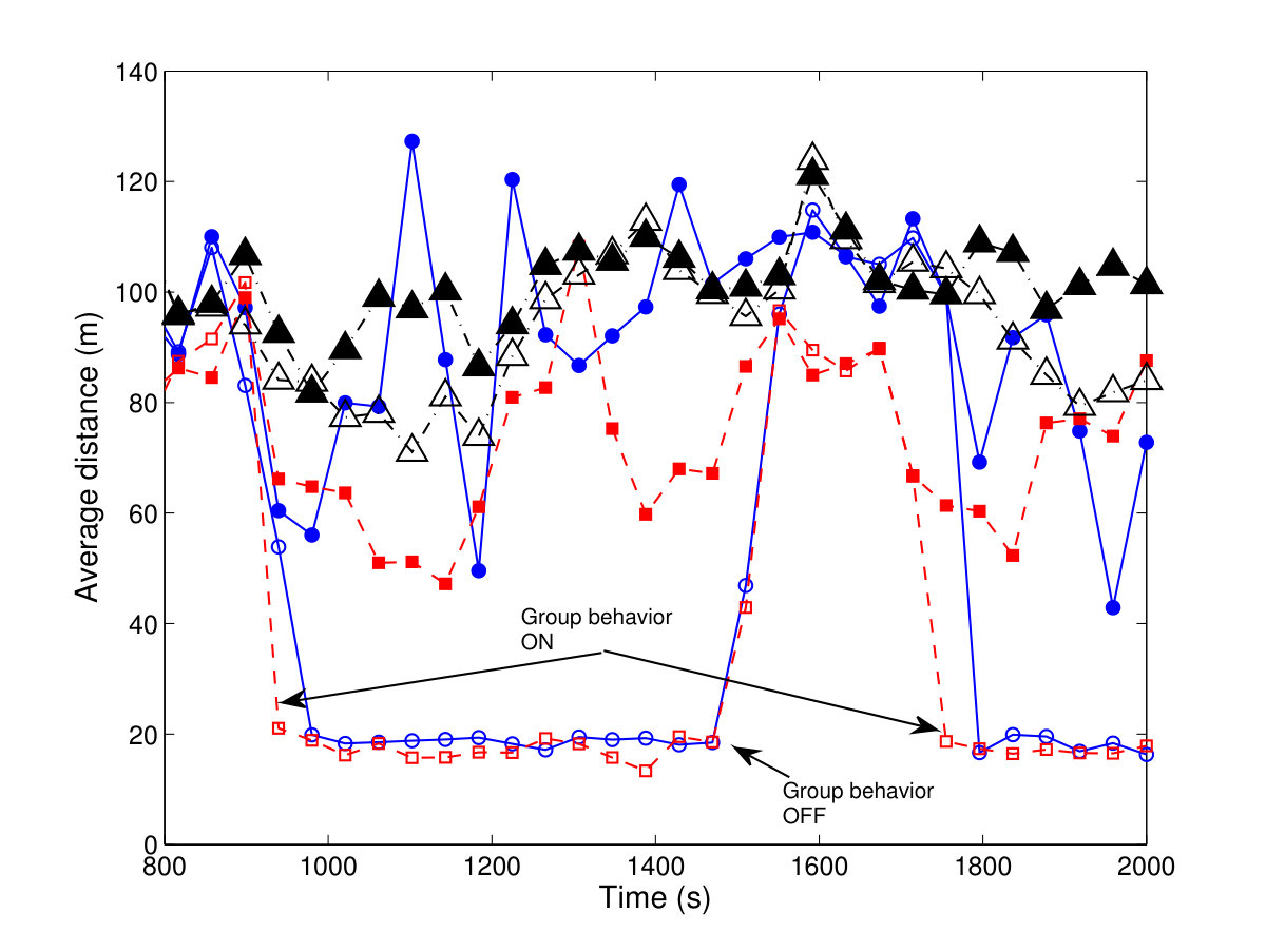 Figure 4
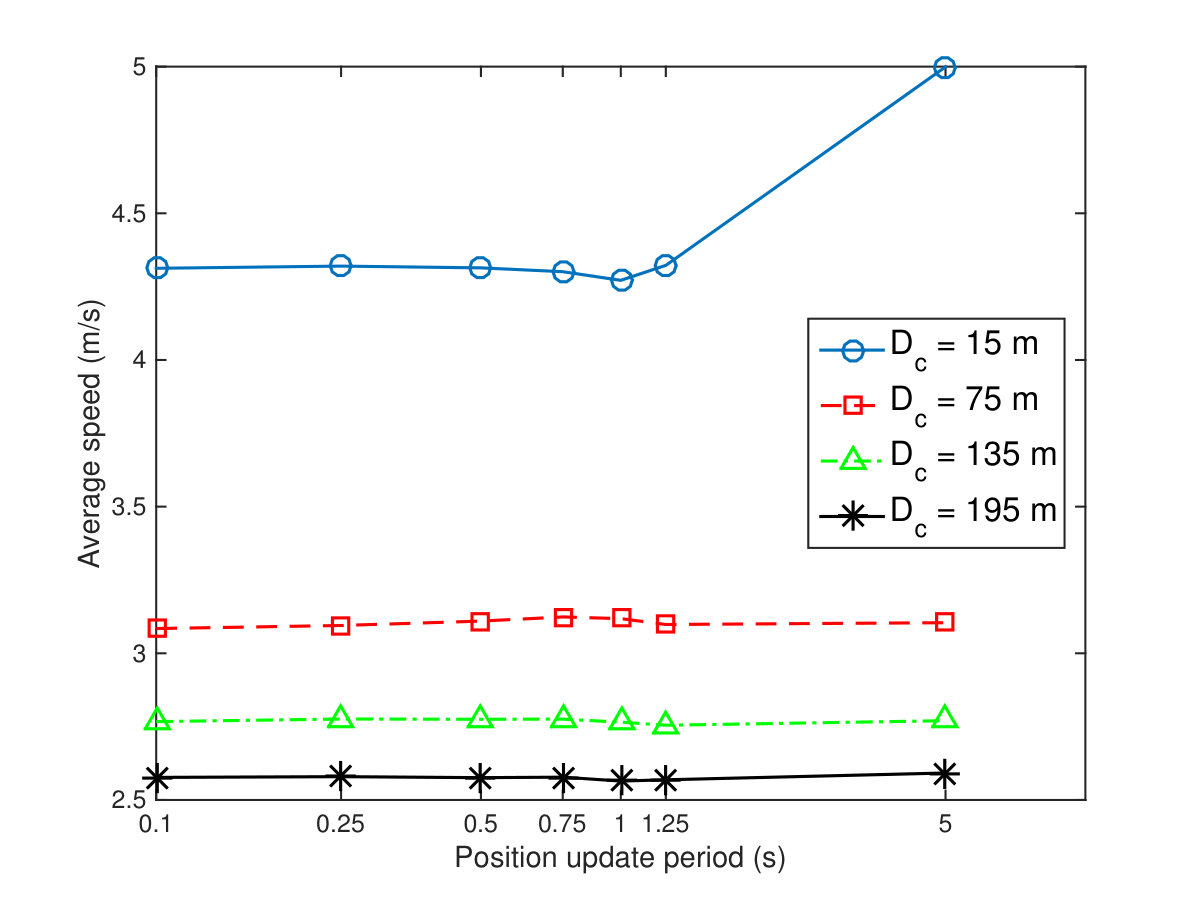 Figure 5
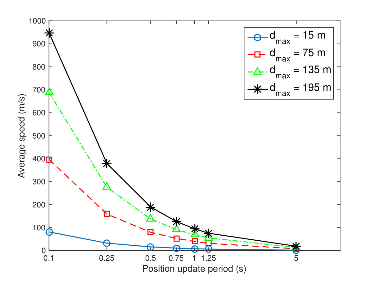 Figure 6
 Figure 7
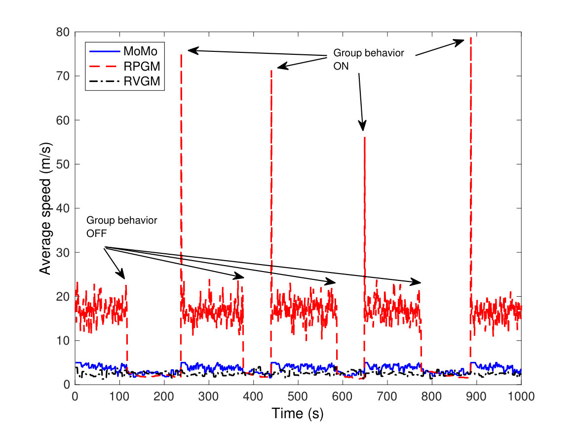 Figure 8
 Figure 9
 Figure 10
 Figure 11
 Figure 12
 Figure 13
 Figure 14
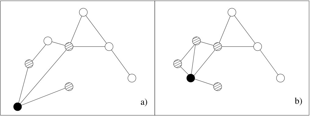 Figure 15
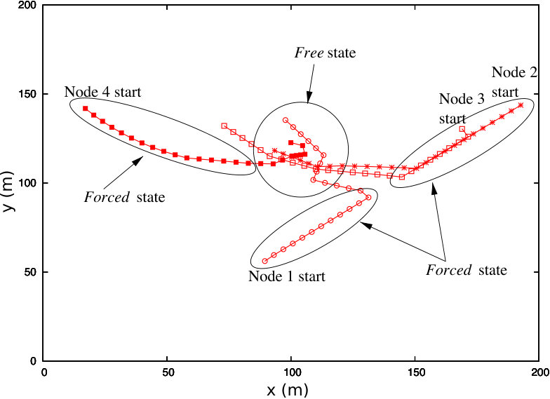 Figure 16
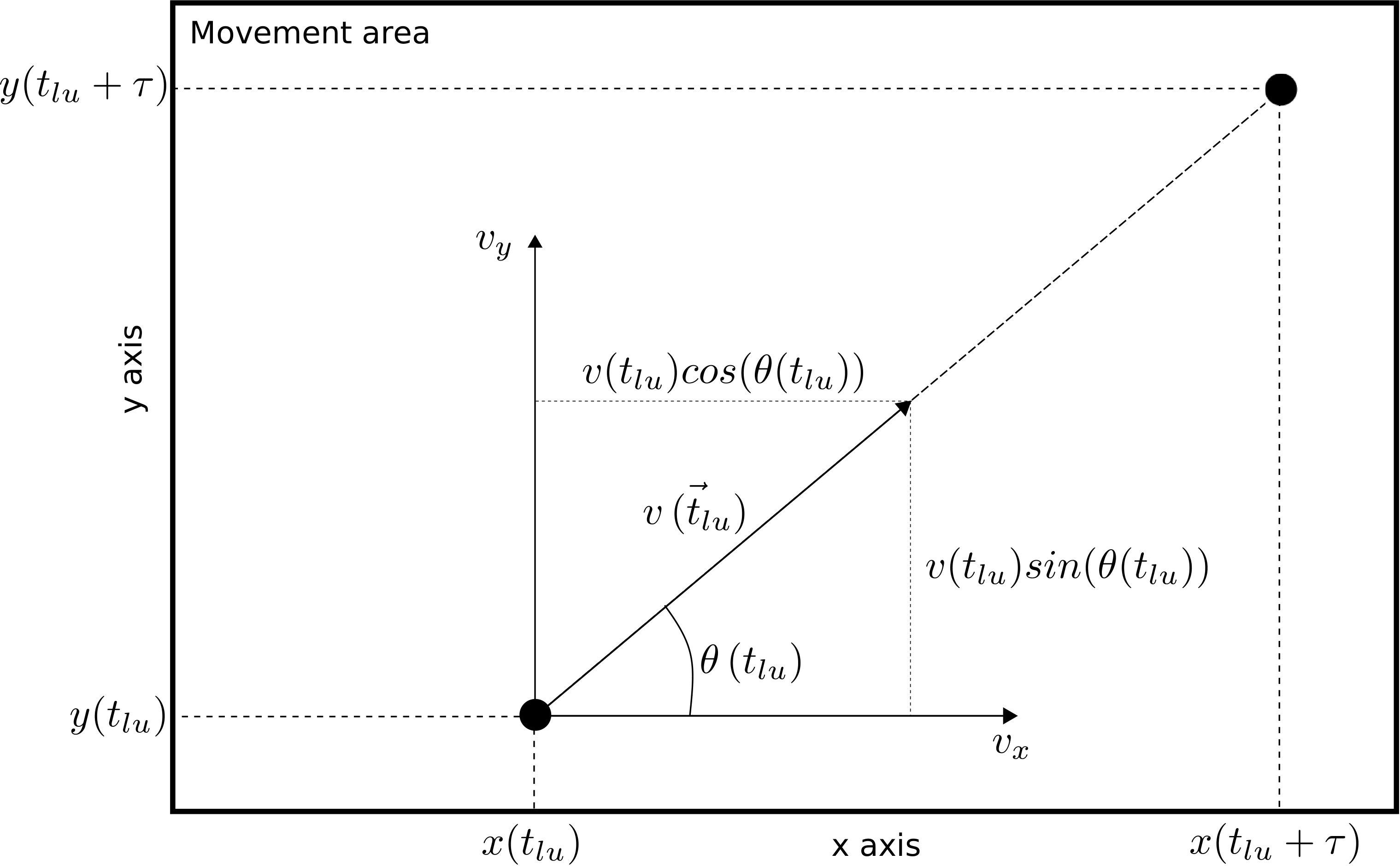 Figure 17
 Figure 18
 Figure 19
 Figure 20
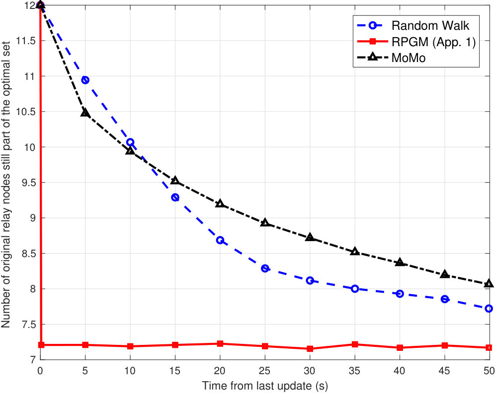 Figure 21
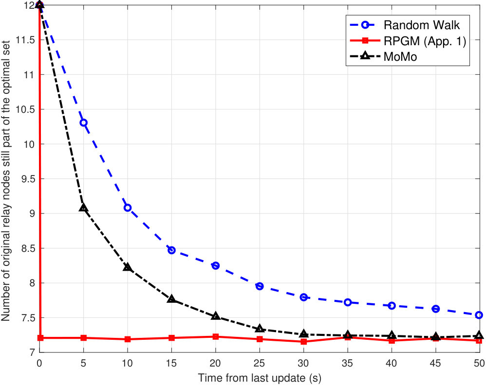 Figure 22
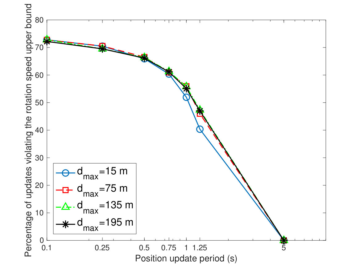 Figure 23
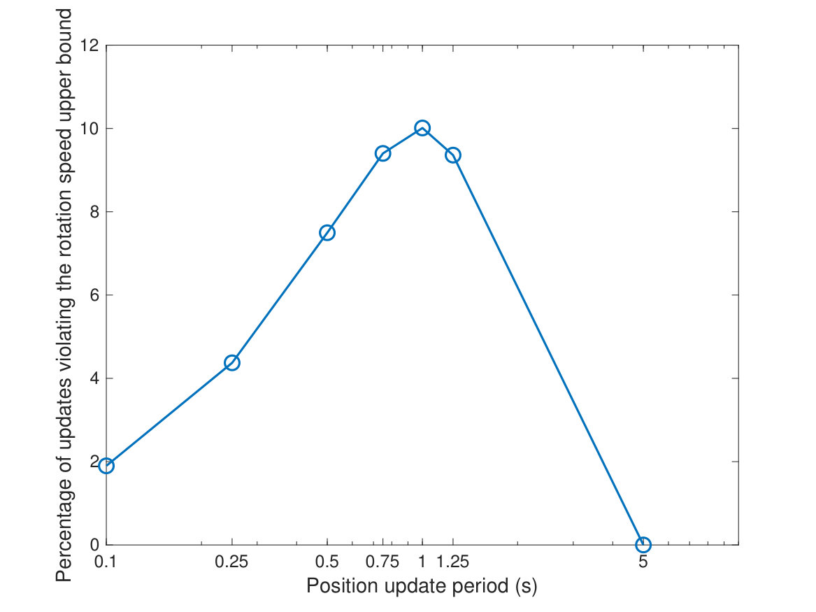 Figure 24
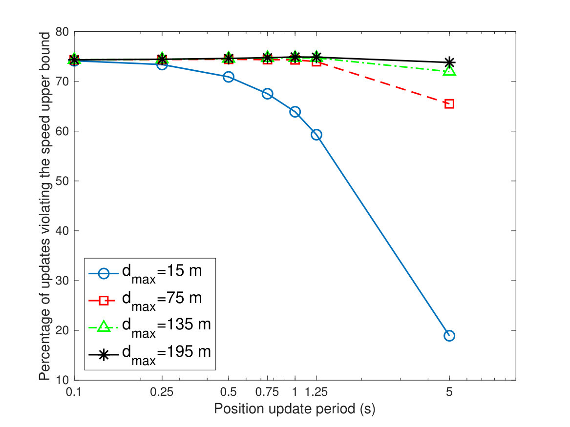 Figure 25
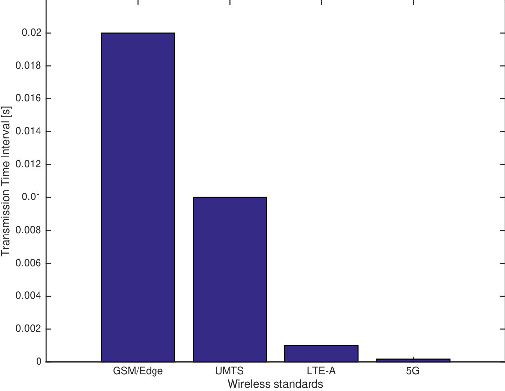 Figure 26
 Figure 27
 Figure 28
| Model | Spatial constraints | Stable group structure | Group destination (Random / Predefined) | Group coordination | Group merge/split | Collision avoidance | Obstacle avoidance |
| RPGM [18] | R | ||||||
| RVGM [19] | R | ||||||
| GFMM [20] | R | ||||||
| MGCM [21] | P | ||||||
| RRGM [22] | P | ||||||
| VTGM [23] | P | ||||||
| CMM [24] / ECMM [25] | P | ||||||
| Mo3 | R/P⋆ | ||||||
| ⋆ Depending on the selected individual mobility model: see Section III-A. | |||||||
| Module | Parameter | Meaning |
|---|---|---|
| Individual Mobility | Speed vector update period | |
| Minimum node speed | ||
| Maximum node speed | ||
| Maximum node linear acceleration | ||
| Maximum node rotation speed | ||
| Maximum elevation angle variation speed | ||
| Correlated Mobility | Speed vector update period | |
| Binding Matrix | Sequence of binding matrices with time of switch (File) | |
| Binding condition threshold | ||
| Grouping condition threshold | ||
| Maximum node speed | ||
| Collision Avoidance | Speed vector update period | |
| Minimum node speed | ||
| Maximum node speed | ||
| Node detection threshold | ||
| Collision risk detection threshold | ||
| Direction variation to address frontal collision risks | ||
| Obstacle Avoidance | Speed vector update period | |
| Obstacles List | List of obstacles with geometrical parameters (File) | |
| Obstacle detection threshold | ||
| Allowed direction margin | ||
| Upper Bounds Enforcement | Speed vector update period | |
| Minimum node speed | ||
| Maximum node speed | ||
| Maximum node linear acceleration | ||
| Maximum node rotation speed | ||
| Maximum elevation angle variation speed |
| Section V-A | Section V-B | ||||
| Mo3 | RPGM | Mo3 | RPGM | RVGM | |
| Groups | 1 | 1 | 4 | 4 | 4 |
| Nodes in the group | N/A | 20 | 4 | 4 | 4 |
| Binding matrix type | Figure 9a | N/A | Figure 4c | N/A | N/A |
| N/A | N/A | N/A | |||
| N/A | N/A | N/A | |||
| N/A | N/A | N/A | N/A | ||
| N/A | N/A | N/A | |||
| N/A | N/A | N/A | |||
| N/A | N/A | N/A | |||
| N/A | N/A | N/A | |||
| N/A | N/A | N/A | |||
| N/A | N/A | N/A | |||
| N/A | (RPGM1) (RPGM2) | N/A | N/A | ||
| N/A | N/A | N/A | N/A | ||
| N/A | N/A | N/A | N/A | ||
| Model | Year | Mobility scenarios | Overall citations | Citations in 2017-2021 |
|---|---|---|---|---|
| RPGM [18] | 1999 | General purpose | 989 | 149 |
| RVGM [19] | 2002 | General purpose | 155 | 17 |
| GFMM [20] | 2009 | General purpose | 17 | 5 |
| MGCM [21] | 2006 | Military pedestrian | 5 | 2 |
| RRGM [22] | 2005 | Security / Search & rescue | 26 | 4 |
| VTGM [23] | 2004 | Military vehicular | 107 | 15 |
| CMM [24] | 2006 | Human social interactions | 254 | 20 |
| ECMM [25] | 2012 | Human social interactions | 32 | 19 |
| SGMM [40] | 2004 | Human social interactions | 52 | 9 |
| BMM[26] | 2006 | General purpose | 20 | 3 |
| BMM-GC [41] | 2013 | Urban mobility | 3 | 1 |
| SIMPS [43] | 2009 | Human social interactions | 59 | 11 |
Peer Reviews
No public reviews on file for this paper yet. If you reviewed it on a platform where reviews are public (OpenReview, ICLR, NeurIPS, ICML), you can paste yours below so the community can read it here.
Code & Models
Videos
No videos yet. Explain this paper in a talk, walkthrough, or lecture? Add one.
\history
Date of publication xxxx 00, 0000, date of current version xxxx 00, 0000. 10.1109/ACCESS.2017.DOI
\tfootnote
This work was partially supported by Sapienza University of Rome, grant nos. RP11916B88A04AE6, RP11816433F508D1, RP11816426A9F174.
\corresp
Corresponding author: Luca De Nardis (e-mail: [email protected]).
Mo3: a Modular Mobility Model for future generation mobile wireless networks
LUCA DE NARDIS1
MARIA-GABRIELLA DI BENEDETTO1
Department of Information Engineering, Electronics and Telecommunications, Sapienza University of Rome, 00184 Rome, Italy (e-mails: [email protected], [email protected])
Abstract
Mobility modeling in 5G and beyond 5G must address typical features such as time-varying correlation between mobility patterns of different nodes, and their variation ranging from macro-mobility (kilometer range) to micro-mobility (sub-meter range). Current models have strong limitations in doing so: the widely used reference-based models, such as the Reference Point Group Mobility (RPGM), lack flexibility and accuracy, while the more sophisticated rule-based (i.e. behavioral) models are complex to set-up and tune.
This paper introduces a new rule-based Modular Mobility Model, named Mo3, that provides accuracy and flexibility on par with behavioral models, while preserving the intuitiveness of the reference-based approach, and is based on five rules: 1) Individual Mobility, 2) Correlated Mobility, 3) Collision Avoidance, 4) Obstacle Avoidance and 5) Upper Bounds Enforcement. Mo3 avoids introducing acceleration vectors to define rules, as behavioral models do, and this significantly reduces complexity. Rules are mapped one-to-one onto five modules, that can be independently enabled or replaced.
Comparison of time-correlation features obtained with Mo3 vs. reference-based models, and in particular RPGM, in pure micro-mobility and mixed macro-mobility / micro-mobility scenarios, shows that Mo3 and RPGM generate mobility patterns with similar topological properties (intra-group and inter-group distances), but that Mo3 preserves a spatial correlation that is lost in RPGM - at no price in terms of complexity - making it suitable for adoption in 5G and beyond 5G.
Index Terms:
Beyond 5G networks, group mobility modeling, mobile wireless networks simulation
\titlepgskip
=-15pt
I Introduction
The design of wireless mobile networks evolved in the last 20 years, from GSM/GPRS to UMTS/HSDPA, from LTE to 5G and the upcoming beyond 5G, along two main trends: increased bandwidth and increased spatial density of wireless devices. Large channel bandwidths require greater physical layer flexibility, so to meet user needs and provide better robustness to channel impairments. One of the physical layer parameters that highlights this trend is the Transmission Time Interval (TTI), defined as the shortest time interval over which link configuration can be adjusted. Figure I shows TTI across four generations of wireless standards (from 20 ms in GSM/Edge [1] to about 0.15 ms in 5G systems [2], [3]). Most likely, TTI will further decrease in beyond 5G, to support ultra-Reliable Low Latency Communications (uRLLC) [4]. \Figuret[width=0.45]./Figures/TTI Evolution of Transmission Time Interval across generations of cellular networks.
Spatial density of wireless devices went from about 1000 devices per square kilometer in GSM, to millions of devices per square kilometer in 5G [5]. The average distance between transmitter and receiver therefore decreased: from hundreds of meters in GSM to a few meters and below in 5G. The steady increase in device density across generations led to major shifts in the design of physical and network layers. At physical layer, signal processing techniques were developed in order to cope with challenging throughput and latency requirements of dense deployments. In particular, beamforming, based on Multiple Input Multiple Output (MIMO), introduced in 3G HSPA and 4G and now fully integrated in 5G, is expected to play a key role in beyond 5G, with the deployment of Massive MIMO [6]. Steering the beam is possible if the relative position of transmitter vs. receiver is known, and requires swift reactions to position changes [7]. At network layer, network topology went from a purely centralized configuration with links spanning over thousands vs. hundreds of meters in 2G vs. 3G, to a mixed nature, with shorter links including both infrastructure to device and Device-To-Device (D2D) connections, as proposed - albeit with limited success - in LTE [8]. Cellular networks in 5G and beyond 5G are expected to take full advantage of direct connectivity between devices [9] and address scenarios - so far restricted to current and legacy Wireless Local Area Networks technologies - in which devices directly exchange data and move in a coordinated manner, although keeping a certain degree of independence in their individual mobility patterns. Examples are:
- •
search and rescue in response to emergency calls or disasters. Best practice rules require operators to work in groups of at least two individuals who keep visual or voice contact with one another [10];
- •
tactical and security teams, with on-demand formation, merging, and splitting of groups [11];
- •
swarms of Unmanned Aerial Vehicles (UAVs) flying in variable formation [12], [13];
- •
cooperative communications in cognitive networks [14].
Note that although distances between devices in a same group may be small (i.e. small micro-mobility, in the order of the meter or sub-meter) the same may not be true for distances covered by groups (i.e. large macro-mobility, in the order of the km). Scenarios can be thus characterized as either mixed macro-mobility / micro-mobility, where groups move over distances much larger than distances within a group, or pure micro-mobility where covered distances are small for both groups and within groups. Moreover, when compared against legacy WLANs, 5G and beyond 5G communications are characterized by less favourable propagation features: the combination of higher operation frequencies and possibly lower radiated power due to the massive number of devices will in fact lead to a reduced radio coverage; cooperative and coordinated mechanisms between devices may be thus introduced [15]. A limited radio coverage also amplifies the impact of device mobility on network connectivity, even when movements are within a short range [16].
Mobility models for 5G and beyond 5G should therefore accurately address both individual and group mobility, independent of distance. This should be done dynamically to also cover situations in which the correlations of mobility patterns of individual nodes may or may not lead to the emergence of groups. Early models of correlated mobility, referred to as reference-based models, are unsuited for the task, since in those models groups are imposed at start, and not dynamically created; for this reason, they are also called group mobility models. Another inherent limitation of these models is the stringent constraints imposed on the mobility patterns of nodes within a group, that limit movements to random variations around either a group reference position (see the seminal Reference Point Group Mobility (RPGM) model [18]), or a group reference speed (see the Reference Vector Group Mobility (RVGM) model [19]). Extensions of the above models introduced new features such as group disbanding and merging, and management of geographical constraints, with no change in the underlying reference-based mechanism. Modelling complex mobility patterns of individual nodes was addressed by so-called behavioral models [26], [20]. These models define rules for the behavior of each node that may include interaction with other nodes and with the environment. For example, two or more nodes may be assigned with a mutual attraction rule that keeps them in close proximity. Collision and obstacle avoidance, an absent component in reference-based models, is obtained by repulsion rules preventing collisions between nodes or with obstacles. In behavioral models, each rule is typically implemented as a force; the intensity of the force is determined based on position, speed and direction of the node itself and of other nodes, and on the position of obstacles. Each force in turn defines an acceleration vector associated with the corresponding rule, and the sum of the acceleration vectors determines the acceleration vector of a node, and by integration over time its speed vector. In behavioural models, groups are not defined at start, but rather emerge from nodes sharing a same set of rules, and having thus similar mobility patterns; each node has however its own speed vector, and thus its individual mobility is modeled without any loss of accuracy caused by the introduction of group mobility. Furthermore, by applying different rules to different nodes, behavioural models can describe correlated mobility scenarios that cannot be addressed by reference-based models, thus providing higher flexibility. Tuning behavioral model to obtain specific spatial correlated mobility patterns is, however, particularly complex, and scenarios that are easily modeled in RPGM become unfeasible with behavioural models [27]. Consider for instance, nodes of a same group that must be within a predefined maximum distance; obtaining this behaviour with behavioural models requires a difficult-to-find balance between mutual attraction vs. repulsion forces, based on the careful selection of several weighting variables [20]. For this reason, behavioural models - although attractive - are unpractical and found little application in wireless networking, where the simplicity of reference-based models was most often preferred over accuracy. This choice becomes however too simplistic in view of 5G and beyond 5G network scenarios, calling for a model that combines the intuitiveness of reference-based models and the accuracy and flexibility of behavioral models.
This paper introduces a new mobility model, called Modular Mobility Model (Mo3), that models, as behavioural models, the mobility of individual agents, but is as straightforward to tune as a reference-based model. In analogy to behavioral models, Mo3 determines the mobility of nodes by defining rules that describe their individual mobility and the effect of mutual interactions as well as with the environment. Mo3, however, does not implement rules as forces. Rather, each rule determines a modification of the speed and direction of movement of a node, without requiring the definition of an acceleration vector and avoiding thus the introduction of weighting variables. The set of rules in Mo3 was defined based on the observation that mobility patterns typically result from modifications to planned trajectories, i.e. a target destination and an initial speed and direction. The deviation from a planned trajectory is usually caused by either voluntary interactions with other agents (correlated mobility) or reactions to external events (collision and obstacle avoidance). Consider for example the case of an individual who visits an art exhibition and is part of a group. At a given point in time, the individual may depart the planned trajectory toward an art piece of interest, due to either voluntary behavior (reunite with the group) or external events (avoiding collision with another visitor or with an obstacle). Note that any modification to speed and direction will stay within the physical limits of the individual. Similar behavior can be observed for fleets of vehicles or animal herds, for example.
Moving from this observation, Mo3 defines five rules: Individual Mobility, Correlated Mobility, Collision Avoidance, Obstacle Avoidance and Upper Bounds Enforcement. Note that the phenomena that determine a given mobility behavior are beyond the scope of this paper; Mo3 takes this information as an input, coded in the Individual Mobility and Correlated Mobility rules settings, and generates accurate and artifact-free mobility patterns, independent of the considered grouping behavior and mobility scale. The Individual Mobility rule, in particular, can be implemented by adopting any existing individual mobility model, to be selected according to the desired mobility behavior.
Table I shows a comparison of Mo3 against existing reference-based and behavioral models, as proposed in [17]. Table I considers the same models analyzed in [17] and includes the features identified as relevant in [17], with the addition of the obstacle avoidance feature. Table I shows that Mo3 provides all the relevant features, and highlights that existing models only provide a subset of the features, in most cases the ones required to model specific mobility scenarios.
The paper is organized as follows. Section II reviews and discusses existing models. Specifically, Section II-A reviews individual mobility models in order to identify suitable candidates for the Individual Mobility rule in Mo3, while Section II-B provides a critical review of the existing correlated mobility models. Section III includes an exhaustive description of the Mo3 model. The section highlights the modular nature of Mo3: each of the rules characterizing Mo3 is paired with a module, that can be replaced without affecting the others. This modularity favours extensions and modifications to Mo3 and, to this purpose, access to an open source software implementation of Mo3 is provided. Section IV provides examples of emulation of existing correlated mobility models using Mo3. Section V compares then Mo3 against other existing models in pure micro-mobility and mixed macro-mobility/micro mobility scenarios. Finally, Section VI draws conclusions.
II Related work on mobility modeling
II-A Individual mobility models
Individual mobility models determine the pattern of each node by varying its speed vector, defined at generic time as: , where is the speed of movement and is the direction of movement, defined as the angle between the axis and the speed vector in the selected coordinate system. The position of a node at any time between two updates of is thus:
[TABLE]
where is the time instant of last speed vector update (see Figure 1).
Models are commonly classified as memoryless vs. memory-based, based on how and are updated.
II-A1 Memoryless mobility models
In memoryless models, updates to values of speed and direction are independent of current and previous values. Well-known memoryless models are:
- •
the Random Walk model, also referred to as Brownian model, widely used to determine the impact of mobility on cellular network performance [28]. The model has the desirable property of leading to a uniform spatial distribution of the position of a node in the movement area. Statistical models of average cell crossing time, average channel holding time, and average number of handovers, were developed using a Random Walk user mobility model [28]. The model was also used in the analysis of mobile ad-hoc routing protocols in presence of node mobility [29].
In the Random Walk model, the selection of a new speed and direction is triggered by either of the following events:
- –
A periodic timer, set to a predefined update period , expires [30];
- –
The node covers a predefined distance [31].
- •
the model proposed by Ko and Vaidya [32] as a simple way to introduce mobility in the performance evaluation of the Location Aided Routing protocol, with no claim for specific advantages over other mobility models. According to the model, a node selects a random direction at simulation start time. The node also selects its speed according to a uniform distribution within a predefined interval , and a distance to be covered at speed , according to an exponential distribution. After covering the distance, new values are selected for , and . When the node hits a boundary of the simulation area, it is perfectly reflected within the area.
- •
the Random Waypoint model, originally proposed in [33]; this model is similar to the Random Walk model, but the trajectory of a node is determined here by a sequence of destination points to be reached. When a node reaches a destination point it pauses for a random time, and then moves towards the next destination point with a new random speed. It has been observed that the Random Waypoint models leads to an uneven spatial distribution of nodes [34], which causes large variations in the average number of neighboring nodes (i.e. nodes within a given distance), especially on the short term [31]. Variations of this model have been proposed to address this issue, such as the Random Direction model, where the node selects a speed vector rather than a destination, and moves according to the selected speed vector until it reaches a boundary of the simulation area when, after a predefined pause time, a new speed vector is selected [34].
All memoryless models share the issue of potentially causing sharp turns and steep variations in speed when a new speed vector is selected, making it impossible to meet upper bounds on linear acceleration and angular speed, and possibly leading to unrealistic mobility patterns.
II-A2 Memory-based models
Memory-based models lead to more realistic patterns by introducing memory in the selection of speed and direction. Well-known models that adopt this approach are:
- •
the Inertia mobility model [35], in which new values for and are selected at each position update with probability , while the current set is kept with probability . Parameter models an inertia that tends to keep the node on the current trajectory: the higher the value of , the lower the probability of selecting a new speed vector. For the Inertia model coincides with the Random Walk model. The Inertia model provides a straightforward mechanism for introducing memory in the selection of the speed vector. New values of and have, however, no correlation with respective previous values. This leads to unrealistic patterns characterized by abrupt turns and speed variations that make it difficult to meet requirements on maximum linear and angular speeds;
- •
the Gauss-Markov model[36], in which the component of the speed vector along direction (with in a two-dimensional space) at time is the outcome of a Gauss-Markov random process , that is a stationary Gaussian process characterized by the following autocorrelation function:
[TABLE]
where and are the variance and the mean of , respectively, and parameter introduces a memory effect. The mobility patterns generated by this model are governed by properly setting the parameter. The Gauss-Markov model provides smoother patterns than Inertia, but still does not provide a straightforward way to meet constraints on maximum speed and rotation in the generation of a mobility pattern. The adoption of a Gaussian probability density function, in particular, may lead to unrealistic values for node speed.
- •
the Boundless mobility model [37], named after the idea of mapping a bidimensional simulation area on the surface of a three-dimensional torus: a node that reaches an edge of the area disappears, and reappears instantaneously on a point on the opposite edge, while keeping the same speed vector. The algorithm for speed and direction update proposed in [37] can be, however, adopted within a traditional bounded movement area as well. In the Boundless model, the speed vector is updated every seconds according to the following rules:
[TABLE]
where:
- –
is the maximum speed;
- –
is the speed variation, uniformly selected at every update time in the interval , where is the maximum linear acceleration allowed for a node, measured in ;
- –
is the direction variation, uniformly selected at every update time in the interval , where is the maximum rotation speed allowed for a node, measured in rad/s.
The Boundless model shares with the Gauss-Markov model the capability of producing realistic movement patterns. The model has, however, the advantage of allowing the introduction of limits on speed, acceleration and rotation speed of nodes, making it easier to achieve realistic mobility patterns that meet predefined upper bounds.
\Figure
t[width=0.48]./Figures/RVGM_T_SU_effect Average distance between nodes in a group of nodes as a function of time in the RVGM model for different values of the update period of the speed vector of standard nodes , assuming a fixed reference speed vector with and . At each update, the speed vector of each node is determined by randomly extracting a speed in and a direction in ; all nodes are placed at the same position at .
II-B Correlated mobility models
Correlated mobility models can be divided into three families: reference-based models, behavioral models, and models based on social network theory [38]. In reference-based models, correlation typically implies the presence of groups; the positions of nodes belonging to a same group is determined as a random deviation from a common reference, defined either as a reference position or as a reference speed vector (see Section II-B1). In behavioral models, nodes select their speed and direction according to predefined rules; in these models, groups naturally emerge from more nodes sharing same rules (Section II-B2). Social network theory models match the mobility patterns to those of people in a community (Section II-B3). Section II-B4 compares the different models and identifies benchmarks for performance evaluation.
II-B1 Reference-based models
The Exponential Correlated Random (ECR) mobility model, proposed in [39], was one of the first models addressing correlated mobility. ECR models the mobility of a group, but not of individual nodes.
The Reference Point Group Mobility (RPGM) model was designed in order to overcome the limitations of ECR, by allowing the description of group as well as individual node mobility within a group [18]. RPGM defines a logical reference point for each group, that often coincides with the position of one of the nodes in the group (group leader), whose movement is followed by all nodes in the group (standard nodes). The path of the group leader is typically generated according to an individual mobility model; for example, the Random Waypoint model (see Section II-A) was used in [18]. The position of standard nodes is generated randomly, according to a uniform distribution for both angle and distance from the reference position of the leader (within ), and is refreshed every seconds. The Structured Group Mobility Model (SGMM) [40] extended RPGM by introducing different statistical distributions for the position of different standard nodes.
In RPGM-based models standard nodes are not associated with a speed vector: their position is in fact only known at each position update at time . In 5G and beyond 5G scenarios, the adoption of a short to match the TTI parameter, leads to erratic mobility patterns for standard nodes, as shown in Figure 2, presenting the patterns generated for a group leader and a standard node in the same group for three different values. Figure 2 highlights that, although on average the standard node follows the group leader for all values, its pattern shows an increasing variability as decreases. Furthermore, as shown in Section V-B3, the maximum speed for a standard node, for small , is about , which leads to unreasonable speeds.
The Reference Velocity Group Mobility (RVGM) model [19] proposed the use of a reference speed vector, rather than a reference position, so that each node has its own speed vector. Here, a random deviation with respect to reference is introduced on the speed vector rather than on the position of standard nodes. The period with which the speed vector of a standard node is updated is an independent factor, that is tuned by the requirements of the mobility scenario. At any instant in time, the position of a node can be determined by a simple calculation based on the current speed vector; this solves the problem of erratic behaviour of standard nodes observed in RPGM, when frequent updates are required. However, RVGM does not provide any mechanism to preserve physical proximity within a group, or to restore it by forcing a standard node to rejoin its group, and this autonomy allows standard nodes to drift away. This eventually leads to a loss of cohesion within groups, as shown in Figure 2. Figure 2 shows the average distance within a group of nodes, as a function of time, for different values of . All nodes are placed in a same position in and, at each update, relatively small deviations from the reference vector are allowed (see caption of Figure 2 for details). Results show that the average distance steadily increases over time for all values, highlighting the loss of physical proximity within the group.
A common trait of reference-based models discussed so far is a static definition of groups, that is no mechanisms are defined to change the composition of groups. A reference-based model that allows group merging and splitting is the Reference Region Group Mobility (RRGM) model [22]. RRGM defines a set of target destinations for groups, and corresponding reference regions surrounding the destinations. The model manages group merging by assigning the same destinations/reference regions to two groups, and group splitting by assigning a new reference region to part of the nodes in a group. The model places however several restrictions on when group merging and splitting can happen in time, and on which groups will be merged or split, as a function of their positions and of the position of the new target destination. Furthermore, the complexity in setting up the model is higher than in RPGM and RVGM, losing the simplicity that is a key advantage of reference-based models.
II-B2 Behavioral models
The concept of behavioral mobility modeling was first adopted in the Behavioral Mobility Model (BMM) [26]. In behavioral models, the mobility pattern of a node is governed by a set of rules, expressed as forces on the node, that is, acceleration vectors. For each force one has an acceleration vector ; the combination of acceleration vectors leads to a global acceleration vector , that in turn determines the speed vector, and eventually the trajectory of the node. The set of rules proposed in [26] determines the behavior of a node with respect to a) node destination, b) surrounding environment, and c) presence of other nodes. The main "desired destination" rule is the Path Following rule, that introduces an acceleration vector towards a preset destination, under a node maximum speed constraint. Environmental rules include Wall Avoidance and Obstacle Avoidance, that generate repulsive forces. Finally, rules that determine the behavior of a node in the presence of other nodes include Mutual Avoidance, avoiding collisions between nodes, and Group Centering and Velocity Matching, forcing nodes to stay close to one another in the space vs. speed domains, and are the behavioral equivalents of RPGM vs. RVGM. An extension of [26], referred to as Behavioral Mobility Model with Geographic Constraints (BMM-GC) [41], provides a more accurate modeling of the interaction with obstacles. Another model adopting a behavioral approach for the interaction between nodes quite similar to [26] is the Group Force Mobility Model (GFMM)[20].
Behavioral mobility modeling was also investigated in [42], where a modular approach is proposed, in which basic rules are combined in order to generate complex behaviors such as group mobility. Basic rules include Seek, Flee, and Arrive for individual mobility, and Pursuit, Evade and Interpose for modeling the interaction between nodes.
Finally, in [43] the rules generating acceleration vectors are based on a sociological analysis of the impact of social ties between individuals on mobility patterns.
A major drawback of behavioral mobility models is their complexity at set-up, due to the need of selecting normalizing and scaling factors to determine the strength of the forces. Furthermore, mobility patterns that are easy to describe in reference-based models, e.g. a maximum distance between nodes in a group, are extremely difficult to describe with rules, as observed in [27].
II-B3 Social network theory models
Studies on the interactions among members of a community inspired a third family of correlated mobility models, based on social network theory [38]. The Community Based Mobility Model (CMM) [24] introduces the concept of Interaction Matrix, with elements indicating the degree of social interaction between any two nodes, and the corresponding inclination to spend time together with a value between 0 and 1. Although CMM and its enhanced version Enhanced CMM [25] are designed for the specific scenario of social human interactions, the concept of the Interaction Matrix can be applied to different mobility scenarios. A similar approach is adopted in Mo3 as part of the Correlated Mobility rule, as explained in Section III-B.
II-B4 Benchmark selection
The comparison in terms of features presented in Table I and the review carried out in this section highlight that a large number of correlated/group mobility models have been proposed through the years; a fair question is thus how to select which models to consider as a benchmark when proposing and evaluating a new model. The proposed selection was based on two factors: the suitability of models to address the same wide range of mobility scenarios targeted by Mo3, and the intuitiveness in describing such scenarios. Based on the review of this Section, one may conclude that models based on social network theory are hardly adaptable to the scenarios identified in Section I. Behavioral models, on the other hand, are potentially capable of addressing any scenario; however, the difficulty in setting them up, preventing their widespread adoption, does not favor their selection as benchmarks. For this reason, the selected benchmarks belong to the reference-based class, as further discussed in Section V: RPGM, by far the most popular and preferred choice for group mobility modeling [44], and RVGM, another general purpose reference-based model. The validity of this selection is also reflected by the impact the selected models on the research community, as measured by the citation indexes of related scientific literature (see Appendix A). \Figuret[width=]./Figures/Figure_Mo3_procedure The Mo3 model. The Mo3 rules are applied sequentially on the speed vector, starting with Individual Mobility, followed by Correlated Mobility, Collision Avoidance, Obstacle Avoidance and finally Upper Bounds Enforcement. Note that the Upper Bounds Enforcement rule takes in input both the output speed vector resulting from the application of the Obstacle Avoidance rule and the current speed vector, in order to ensure that the cumulative modifications introduced by the first four rules do not exceed the maximum allowed variations for linear and angular speeds.
III The Mo3 model
Mo3 models the mobility of each node by applying five rules: Individual Mobility, Correlated Mobility, Collision Avoidance, Obstacle Avoidance and Upper Bounds Enforcement. The peculiar and novel aspect of Mo3 consists in its modularity. Each rule is implemented in a dedicated module, and each module can be replaced without affecting the other modules, providing thus ample possibility to expand Mo3 and tailor it for new mobility scenarios that may emerge in the future. Furthermore, depending on the considered mobility scenario, modules can be independently turned on and off, and can operate with different update periods.
The modular nature of Mo3 also allows to introduce mobility in the third dimension for selected rules; Individual Mobility, Correlated Mobility and Upper Bounds Enforcement rules, in particular, support tridimensional mobility, while the introduction of this feature in Collision Avoidance and Obstacle Avoidance rules is left for future work. When tridimensional mobility is selected, the modules corresponding to rules that do not support this feature can be selectively disabled.
Mo3 supports tridimensional mobility by adopting a spherical coordinate system, where the speed vector associated to a node is represented as a triplet : and have the same meaning as in the bidimensional speed vector introduced in Section II-A, while indicates the elevation angle, defined as the angle between the speed vector and the plane, as shown in Figure III, where the dependence on time is omitted to simplify notation. \Figuret[width=0.45]./Figures/3Dvector.eps Definition of the speed vector in three dimensions. Correspondingly, (1) becomes:
[TABLE]
where and are defined as in (1), , while .
A bidimensional mobility scenario can be modeled by setting ; in this case (4) coincides with (1) for any arbitrary choice of . This scenario is considered throughout the paper, in order to simplify the graphical representation of patterns and allow for comparison with the bidimensional RPGM and RVGM models adopted as benchmarks; examples of patterns in a tridimensional mobility scenario are however provided in Sections III-A and III-B.
In Mo3, at each mobility update the speed vector for a generic node is modified by sequentially applying each of the five rules. The first rule to be applied takes thus as an input the current speed vector ; the resulting speed vector is transferred to the second rule, and so on; when one module is not active or skips a given mobility update, the speed vector is transparently moved from its input to its output, without modifications. The output of the last rule is the new speed vector .
Note that the order of application defines a hierarchy between the rules: rules applied later prevail on those applied earlier. The order selected in this work is the following: 1) Individual Mobility; 2) Correlated Mobility; 3) Collision Avoidance; 4) Obstacle Avoidance; 5) Upper Bounds Enforcement. The order was determined as a reasonable model of the behavior described in Section I for a group of people, a herd of animals, or a fleet of vehicles: the need to meet constraints caused by correlated mobility supersedes the node’s individual mobility model, and in turn the need to avoid collisions with other nodes and with obstacles takes precedence on e.g. keeping up with a group. Finally, the enforcement of bounds on linear and angular speeds prevails on everything else, even if this might result in a failure to avoid a collision. The resulting model is presented in Figure II-B4. Figure II-B4 highlights the special role of the Upper Bounds Enforcement rule, that compares the speed vector , resulting from the application of the first four rules, with the current speed vector , and ensures that the cumulative modifications applied to do not exceed the maximum allowed variations for linear and angular speeds. As a final note on the selected order, one might argue that establishing a hierarchy between collision avoidance and obstacle avoidance is somewhat arbitrary; however, as it will explained in Sections III-C and III-D, the Collision Avoidance and Obstacle Avoidance rules are designed to operate on mutually different mobility parameters, so to mitigate the risk of conflicts between the corresponding corrections.
The five Mo3 rules and corresponding modules are described in sections III-A to III-E; section III-F describes the setup procedure and summarizes the model input parameters, divided by module. Finally, Section III-G provides information on how to access an open-source software that implements the model.
Note that the output speed vector of each module is labelled with a corresponding superscript, as shown in Figure II-B4. In the following, superscripts will be however dropped when possible, in order to simplify the notation, in which case the input speed vector is indicated as , and the corresponding output as .
III-A Individual Mobility
Any individual mobility model can be adopted in Mo3 to implement the Individual Mobility rule: the choice only depends on the specific mobility scenario under consideration, that defines the desired behavior for the nodes in the network.
The model adopted in this works was selected based on the review carried out in Section II-A. The review highlighted that memoryless models typically lead to unrealistic mobility patterns due to the sudden changes in speed and direction. Among the memory-based models, the Boundless model emerged as a good compromise between accuracy and flexibility in providing realistic mobility patterns, as shown in Figure 3, presenting a node mobility pattern obtained with the Boundless mobility model in an area of , with , , and . An individual mobility model inspired by the Boundless model was thus adopted throughout this work, and in particular in the performance evaluation carried out in Section V.
The model proposed in this work differs from the Boundless model under two aspects: first, the minimum speed, that is always set to 0 in (3) is explicitly defined as in the following; second, the model supports tridimensional mobility by means of the following speed vector update rules, that extend (3):
[TABLE]
where , and are defined as in (3); is the elevation angle variation, randomly selected at every update according to a uniform distribution defined on the interval , where is the maximum elevation variation speed allowed for a node in rad/s. An example of tridimensional patterns achievable with this rule is presented in Figure 5.
\Figuret[width=0.45]./Figures/3DpatternsFree.eps Example of patterns in three dimensions achievable with the Individual Mobility rule with , , , and . It is worth reiterating that all the other rules defined in Mo3 and described in the following subsections operate independently from the selected individual mobility model.
The Individual Mobility rule is applied with a period .
III-B Correlated Mobility
The Correlated Mobility rule relies on three key concepts: binding, binding condition and grouping condition. The concepts are defined as follows, for a generic node :
- •
A binding is a relation between the mobility patterns of two nodes. If a binding exists between the mobility patterns of and of a second node , is referred to as mate of node . The mates of nodes form its so-called binding set ; is by definition a member of . The size of is indicated with .
- •
For each node , the following binding condition, inherited from the model proposed in [45], is defined:
[TABLE]
where is the distance between nodes and , and the distance is a tunable threshold. If the binding condition in (6) is satisfied, is said to be connected to . Note that will always be connected to itself, since , and the corresponding binding condition is trivial. The set of mates is connected to is referred to as its connected set , of size .
- •
A grouping factor is defined as:
[TABLE]
and the following grouping condition is defined on :
[TABLE]
where the threshold is also a tunable parameter111For a node that moves independently of any other node one has and at all times; in this case by definition, and the grouping condition in (8) is always satisfied..
The Correlated Mobility rule is applied to each node with period . The application of the rule consists of the following algorithm:
determine the binding set based on the existing bindings; 2. 2.
determine the connected set , by checking the binding condition for each ; 3. 3.
evaluate and determine whether the grouping condition is satisfied. If this is the case, set the node in a Free state and set ; if not, set the node in a Forced state, and take a corrective action by choosing so that the grouping condition can be satisfied in the shortest possible time.
More details on the definition of bindings, on the corrective action associated with the Forced state, and on the definition of connectivity are provided in the three following subsections.
III-B1 Binding definition
The bindings between nodes are defined by providing a binding matrix of size , where is the total number of nodes in the network, defined as follows:
[TABLE]
where
[TABLE]
By definition, . On the other hand, bindings are not necessarily symmetric, so one can have for .
The dependence on time of the elements of allows to define dynamic bindings, a feature lacking in most models reviewed in Section II-B. The impact of dynamic bindings as provided by Mo3 will be analyzed in Section V-B; out of simplicity, in the remainder of this Section a static case where bindings do not vary in time will be considered, and the dependence on will be dropped.
The binding matrix provides an intuitive representation of the correlation between mobility patterns: for a given node , the size and the composition of its binding set can be immediately identified by inspecting the -th row of . A few notable configurations for can be identified:
- •
– each node is only bound to itself; this corresponds to a complete absence of correlation. Each mode will move according to its own individual mobility model;
- •
is a diagonal block matrix with the generic diagonal block equal to 222 is defined in linear algebra as an matrix of all ones. – each block defines a group as defined in the reference-based models reviewed in Section II-B.
Figure 4 presents a few examples of binding matrices falling into one of the two above categories (see Figures 4a-4e). Note that mixed scenarios, where some nodes adopt a group mobility behavior while the remaining ones move according to an individual mobility model, can be described by simply defining diagonal blocks of size 1, as shown in Figure 4e. The flexibility provided by the binding mechanism allows, however, to model any configuration, including those not belonging neither to individual mobility nor to group/mixed mobility as described above. This provides Mo3 with the capability of mimicking most of the correlated mobility models introduced in the literature. An example of this feature is shown in Figure 4f, presenting a binding matrix that defines three groups, formed by a) nodes , , , b) nodes , , and c) nodes , . The binding matrix however also introduces inter-group bindings between nodes , and , emulating the feature of Group Coordination, as defined in [17]. The capability of Mo3 to emulate other models is further discussed in Section IV.
III-B2 Corrective action for a node in Forced state
When is in Forced state, the following corrective action is taken:
select the closest mate not part of , defined as:
[TABLE] 2. 2.
select , and as follows:
[TABLE]
[TABLE]
[TABLE]
where the operator returns the principal value of in .
Equations (12), (13) and (14) ensure that node adopts the speed vector that will reach the current position of the selected mate in the shortest possible time. The pair identifies in fact the direction of the vector centered in the current position of node and pointing to the current position of node . The equations also address the case of bidimensional mobility, since in this case and thus ; is therefore the direction from the current position of node , , to the current position of node , . Figure 5 shows an example of application of the Correlated Mobility rule in the case of a node (black circle) with a binding set of size , with ; arcs between nodes indicate connectivity as defined in (6). In Figure 5a the size of the connected set (striped circles) for the node leads to a grouping factor . The grouping condition is thus not satisfied, and the node moves toward the closest mate among those it is not connected to (white circles), until the condition is satisfied (Figure 5b, where and ).
An example of the movement patterns obtained in a bidimensional mobility scenario by applying the Correlated Mobility rule for a single group of 4 nodes, corresponding to the binding matrix in Figure 4b with , is presented in Figure 5, that also highlights the state of each node (Free vs. Forced). An example of movement patterns obtained in a tridimensional mobility scenario is shown in Figure 5.
\Figure
t[width=0.45]./Figures/Mo3_pattern Mobility patterns obtained by applying the Correlated Mobility rule for a single group of 4 nodes. As nodes start from random positions, the grouping factor is below the threshold for all of them. Nodes thus start moving in Forced state; as soon they achieve they switch to Free state. The patterns were obtained using the Individual Mobility rule proposed in Section III-A and the following settings: area size , , , , , , , , .
\Figure
t[width=0.45]./Figures/3DpatternsCorr.eps Mobility patterns in three dimensions obtained by applying the Correlation Mobility rule for a single group of 4 nodes and the following settings: area size , , , , ,, , , , .
III-B3 Definition of connectivity and meaning of
The definition of connectivity, and the corresponding meaning of the threshold , depends on the mobility scenario; the binding condition adopted in Mo3 is general enough to address a wide range of scenarios. Two possible examples are the following:
- •
connectivity related to radio communications - in this case two mates will be considered as connected if they can communicate through a direct radio link (physical layer connectivity), and will be set depending on the radio coverage;
- •
connectivity based on a radio-independent parameter - for example, if a group corresponds to a security team, connectivity may correspond to physical visibility: a team member will be connected to another if they are in line of sight.
III-C Collision Avoidance
Collision avoidance in Mo3 aims at predicting potential collisions, based on the positions and speed vectors of nodes, and taking a corrective action before they happen. A corrective action could in general include a change in both speed and direction of a node; in Mo3, however, the Collision Avoidance rule introduces modifications to speed only, unless a change of direction is absolutely necessary to avoid a frontal collision 333The probability of a frontal collision is negligible when speeds and directions are selected randomly. For this reason, this issue is addressed in Appendix B, focusing in this Section on the more common case of collisions that are not frontal.. This choice has two justifications: first, it allows to avoid collisions with other nodes without changing course, which is a reasonable model of what happens in real world mobility; secondly, it minimizes the conflicts between the corrections introduced by Collision Avoidance vs. Obstacle Avoidance rules. As it will be detailed in Section III-D, in fact, the Obstacle Avoidance rule only operates on direction of movement and not on speed.
The core idea in the Collision Avoidance rule proposed in Mo3 is to identify collision risks based on the current trajectories of nodes rather than on their mutual distance; for example, two nodes that move on parallel lines will never trigger a collision risk alert in Mo3, regardless of their distance. A collision risk is in fact identified for a node only if its current speed vector will place it within less than meters from any other node when either of them reaches the location where their paths would cross (crossing point). An example of a scenario potentially causing a collision risk is presented in Figure 3. Figure 3 highlights for either node the positions that would trigger a collision risk alert when the other node is at the crossing point, corresponding to the segment of its planned path that falls within a circle of radius centered on the crossing point.
The Collision Avoidance rule is applied for each node with period .\Figuret[width=0.45]./Figures/Figure_CA_exampleExample of possible collision risk considering two nodes and with crossing paths. A collision risk is detected if the current speeds of the two nodes would lead either node to occupy any location in the segment of its own path highlighted in bold when the other node is at the path crossing point; the length of each segment is equal to . A brief description of the algorithm implementing the rule is provided in the following; details on the computations carried out at each step are provided in Appendix B.
The output speed for node is determined as follows:
- •
Path crossing identification - trajectories of all nodes within a distance from are analyzed, and nodes that are on trajectories crossing the current trajectory of are added to the set of Path Crossing Nodes ;
- •
Speed bounds determination - for each node , the range is determined for , that guarantees that when either node reaches the crossing point; a corresponding constraint is defined, expressed by the inequality ;
- •
Collision avoidance - the set of constraints on the new speed determined at the previous step is analyzed in order to determine whether the corresponding system of inequalities can be solved. As shown in Appendix B, the analysis will lead to one of three possible outcomes:
no collision risk is identified, and no action is taken, leading to ; 2. 2.
a collision risk involving one or more nodes in is identified, and can be addressed by choosing a ; 3. 3.
a collision risk involving one or more nodes in is identified and cannot be addressed: the that best mitigates the risk is selected, and a further attempt to fully address it will take place at the next application of the Collision Avoidance rule.
Figure 6 shows the probability of a collision risk for a node, estimated as the average frequency of observed collision risks in generated mobility patterns, as a function of in a scenario considering nodes moving independently in an area . Figure 6 highlights that the Collision Avoidance rule is effective in mitigating the risk of collisions. As the required increases, the probability of a collision risk increases as well, since the condition to be met is harder and harder to satisfy; nevertheless the application of the Collision Avoidance rule reduces in all cases the probability of a collision risk by about one order of magnitude.
III-D Obstacle Avoidance
Several approaches to obstacle avoidance were proposed in the past. The Obstacle Model [46] was designed to model the movement of people walking around and through buildings; it defined obstacles shaped as polygons, and restricted nodes to move on a set of paths equidistant from obstacles, determined by partitioning the movement area according to a Voronoi diagram, with the corners of obstacles as location points for the diagram. An evolution of this model was proposed in [47], in which obstacles were defined as rectangles of arbitrary size and orientation, but nodes’ movement patterns were still restricted to a set of paths between obstacles, albeit richer than the one obtained in [46]. GFMM [20] adopted instead a behavioral approach, that allowed nodes to occupy any position in areas not covered by obstacles, by defining a repulsion force from obstacles, but without providing a mechanism to define obstacles of arbitrary size and shape.
Mo3 introduces an Obstacle Avoidance rule that shares with [46], [47] a geometrical approach to the definition of obstacles, but provides complete freedom of movement for nodes around and between obstacles as in [20]. Section III-D1 introduces the basic obstacle shapes available in Mo3 and how they are defined, while Section III-D2 describes how obstacles are detected and avoided by nodes in Mo3.
III-D1 Obstacle definition
Obstacles in Mo3 can take the basic shapes of either a rectangle or an ellipse444Both ellipses and rectangles can only be defined with one axis/side parallel to the horizontal axis of the movement area. The extension to shapes with arbitrary rotation is left for future work.. The obstacles are defined by providing the geometric information needed to place them in the movement area, that is: 1) the coordinates of the center and the length of horizontal semi axis and vertical semi axis for an ellipse, and 2) the coordinates of the center and the length of horizontal and vertical sides for a rectangle. Obstacles with more elaborate shapes can be obtained by combining (possibly overlapping) basic shapes.
The choice of defining obstacles over a set of basic shapes allowed to define an Obstacle Avoidance rule based on a geometric approach, as explained in the following subsection.
III-D2 Obstacle avoidance rule
Since a change in speed would not avoid a collision with an obstacle, the Obstacle Avoidance only modifies the direction of movement. As anticipated, this choice has also the advantage of decoupling the corrections applied by this rule from those introduced by the Collision Avoidance rule, mitigating the risk of conflicts.
The Obstacle Avoidance rule is applied for each node with period , taking into account all obstacles within a distance from the node. The algorithm that determines the new direction is as follows:
- •
For each obstacle , determine whether the minimum distance from to any point in is lower than . If this is not the case, ignore it, otherwise find the two angles and that determine the range of directions that would lead to a collision, based on the geometry of the obstacle and the current position of (see Appendix C for details), and label such range as forbidden555The concept of forbidden range of directions is similar to the one of obstruction cone introduced in [46]. However, in [46] the concept was adopted only to model radio blockage, and only for rectangular obstacles..
- •
Determine the range of allowed directions as the complement to of the union of all the forbidden ranges determined at the previous step, and compare it with the current direction . The analysis can lead to either of the following outcomes666The possible outcomes are defined assuming that the range of allowed directions is not empty. The case where no allowed direction exists corresponds to a scenario where a node is surrounded in all directions by obstacles at distance shorter than , that is extremely unlikely in common mobility scenarios.:
is within the allowed range: no collision risk is identified, and no action is taken, leading to ; 2. 2.
is not within the allowed range: a collision risk involving one or more obstacles is identified, and is addressed by selecting a defined as follows:
[TABLE]
The angle identified by (15) is the one minimizing the correction introduced on the input direction, shifted by a small margin that ensures that will not touch the obstacle at the tangent point.
An example of the application of the Obstacle Avoidance rule for a generic node is presented in Figure III-D2, showing a scenario with three obstacles: a rectangle, labeled with , an ellipse (), and a circle (). Obstacle is excluded from the computation of the forbidden ranges, since it is not within a distance from . The allowed range , obtained as the complement to of the union of the forbidden ranges determined by obstacles and , is identified by the green shaded area. A collision risk is identified, since , and in the considered scenario is selected to address the risk.
\Figuret[width=0.45]./Figures/Figure_OA_example.eps Application of the Obstacle Avoidance rule for a node in presence of three obstacles: a rectangle, labeled with , an ellipse (), and a circle () at distance larger than ; the allowed range of directions is highlighted with a shade of green. A collision risk is detected with the rectangle, and is adopted to address it. Several examples of mobility patterns obtained using the Obstacle Avoidance rule are presented in Figure 7. Figure 7a and Figure 7b consider two scenarios with 2 obstacles, respectively a circle and a square with vs. a rectangle and an ellipse with . Figure 7c and 7d highlight the impact of , by showing the patterns obtained in the same scenario with a single obstacle and for vs. over a long observation time, that allows for an almost full coverage of the movement area by the node. A comparison between Figure 7c and 7d shows that collisions are prevented in both cases, but a larger allows an early application of the Collision Avoidance rule, resulting in trajectories farther away from the obstacle compared to those obtained for a small , as highlighted by a lower density of trajectories in close vicinity to the obstacle in Figure 7d.
The Obstacle Avoidance rule also allows to define pathways and corridors, by delimiting them with properly placed obstacles, thus implementing the spatial constraint feature introduced in [23] as part of the definition of the Virtual Track Group Mobility (VTGM) model, and listed in [17] as a desirable feature for a mobility model. An example of a mobility pattern obtained by taking advantage of such feature is presented in Figure 7. \Figuret[width=0.45]./Figures/Figure_OA_spatial_constraints.eps Example of a mobility pattern for a network of nodes in presence of spatial constraints, defining a set of hallways in a room. Mo3 settings used to generate the pattern were as follows: , , , , , and .
Finally, the rule can be also used to ensure that nodes remain within the boundaries of the movement area. In most implementations of mobility models this is obtained by adopting a perfect reflection law: nodes hitting a side of the area rebound with same speed and symmetric direction with respect to the normal to the side. The implementation of Mo3 made available in [48] supports this approach as well. A smarter solution to this issue can be however adopted by introducing four extremely narrow rectangular obstacles that delimit the movement area. A comparison between the patterns obtained with the two approaches is shown in Figure 8, highlighting the smoother patterns obtained when the Obstacle Avoidance rule is used.
III-E Upper Bounds Enforcement
The Upper Bounds Enforcement rule is derived from the approach proposed for the Boundless model in [37] to limit the linear acceleration in a range and angular speed in a range . At each update, the updated speed vector for the node under consideration, obtained after the application of the Individual Mobility, Correlated Mobility, Collision Avoidance and Obstacle Avoidance rules, is compared to the original speed vector in order to determine the following variation factors:
[TABLE]
These factors will be compared with the maximum variation allowed by the upper bounds on linear acceleration, rotation speed and elevation variation speed, determining the final speed vector . One has for the speed :
[TABLE]
where is the time elapsed from the previous mobility update, as already defined in Section II-A777In a discrete implementation of the model, with position updates every , one has . Oppositely, if the position update is triggered on demand, measures the time elapsed from the last position update..
For the direction, one must consider the boundary between and in the computation. Let us focus on cases where a violation occurs, corresponding to . For the case one can introduce the logical condition:
[TABLE]
that determines as follows:
[TABLE]
For the case , one has the following logical condition:
[TABLE]
that determines as follows:
[TABLE]
In cases where there is no violation, corresponding to , no correction is needed, and thus .
In the case of the elevation angle there is no boundary condition to be considered, and the output elevation angle is determined as:
[TABLE]
The following observations hold for the Upper Bounds Enforcement rule:
the rule can be used to introduce a memory effect and enforce bounds in Individual Mobility models that do not provide such features natively; 2. 2.
the rule is mandatory also when the Individual Mobility model has built-in upper bound enforcement, as is the case for the Boundless model, because the Correlated Mobility, Collision Avoidance and Obstacle Avoidance rules may modify the speed vector in a way that would cause violations; 3. 3.
in order to ensure that bounds are never violated, the period of execution of the Upper Bounds Enforcement rule, , shall be selected equal to or lower than the minimum update period adopted for the other four rules; 4. 4.
the enforcement of the bounds in (17)-(21) may alter the speed and direction selected as a result of the application of other rules, and in particular of the Collision Avoidance and Obstacle Avoidance rules. In most cases, these alterations will be compensated in subsequent mobility updates, but from time to time they may result in a failure to avoid a collision. Such an event is part of the modeling approach adopted in Mo3: no matter what the mobility scenario under consideration (pedestrian, vehicular, aerial, etc.) collisions do happen in the real world, and Mo3 covers this possibility.
III-F Model setup
The setup procedure for Mo3 can be summarized as follows:
define the number of nodes; 2. 2.
define the coordinate ranges , and in the tridimensional case, determining the movement area (2D case) or space (3D case); 3. 3.
generate or load coordinate sets within that will set the initial position of the nodes. Note that if the Obstacle Avoidance rule is enabled in the bidimensional case, and obstacles are introduced in , the initial positions must be set ensuring that no node is placed inside any region of occupied by an obstacle; 4. 4.
generate or load sets of speed, direction and elevation values, defining the initial speed vectors of the nodes.
Starting from the initial state resulting from the procedure above, Mo3 will periodically update the speed vectors of the nodes, according to the input parameters set for the five modules that compose the model. Table II provides the full list of parameters888The set of parameters required for the Individual Mobility module might change if an individual mobility model different from the one proposed in Section III-A is adopted., indicating for each of them which modules they refer to, and whether they are provided in a configuration file. Table II shows that setting up the model is pretty straightforward: Mo3 does not require normalizing coefficients and weights as behavioral models do, and all parameters have a clear relation with the desired spatial properties for the mobility patterns. In addition, the mobility patterns generated by RPGM can be emulated by activating only the Individual Mobility, Correlated Mobility and Upper Bounds Enforcement modules, with a comparable set-up complexity.
The position of each node will be then updated, typically every seconds, by adding to the previous position the displacement in , and determined by the node’s speed vector.
III-G Availability
The Mo3 model was implemented in Matlab. The software includes a main script performing the setup procedure described in Section III-F and a set of supporting functions implementing each of the modules defined in Sections III-A to III-E. The code is available for download under an open source license from a dedicated GitHub repository [48]. The repository also includes an implementation of a subset of the Mo3 modules for the OMNeT++ [49] discrete event simulator; see Section V-A for details.
IV Using Mo3 to emulate other correlated mobility models
The flexibility provided by the combination of the Individual Mobility and Correlated Mobility rules allows Mo3 to emulate other correlated mobility models. An exhaustive comparison with the most popular group mobility model, that is RPGM, will be carried out in the next two sections; this section focuses instead on other correlated mobility models that do not fall in the group mobility category as defined in Section II-B. Mo3 can effectively emulate these models by adopting an asymmetric Binding Matrix, as anticipated in Section III-B.
Three notable correlated mobility models, all proposed in [50], will be considered in the following: the Pursue, Column and Nomadic Community mobility models.
IV-A Pursue model
The Pursue model describes a scenario where a node (the target) moves independently of any other node, and is pursued by the other nodes.
This model can be easily emulated by adopting the binding matrix shown in Figure 9a, where node is the target and moves independently from the others; correspondingly, row of the binding matrix is equal to the same row in the identity matrix. All remaining nodes are pursuers, and have thus a binding at position of their row. The aggressiveness of the pursuers in following the target can be tuned by properly setting the distance in (10): the lower , the more aggressive the pursuers will be.
IV-B Column model
In the Column model the nodes move in line, with some degree of liberty in deviating from regular spacing.
This model can be emulated by adopting the binding matrix shown in Figure 9b: node will set the pace by deciding freely speed and direction, while each node from to will follow the node before it: as a result, in the row corresponding to the generic node a binding is present in position . By adopting a speed range leading to a relatively fast movement for node , nodes will tend to organize in a line following the leader. The degree of liberty in deviating from this behavior defined in the Column model can be modeled and tuned by properly choosing the distance: a larger distance will guarantee more freedom for the nodes to deviate from the line formation.
IV-C Nomadic community model
The Nomadic community model describes the mobility of a population that alternates moving phases, during which the whole population moves from one area to another, to stationary phases, in which the population members roam freely in an area. As suggested in [50], the model is suitable for describing the movement of security patrols or search & rescue teams, as well as the movement of herds of animals.
The model can be emulated in Mo3 by adopting a time varying binding matrix. The two phases can be in fact modeled by periodically switching between the two binding matrices shown in Figures 9c (moving phases) and 9d (stationary phases) The binding matrix in Figure 9c elects node as the community leader, defining the path toward the area where the next stationary phase will take place. Note that the Correlated Mobility rule introduced in Section III-B will ensure that the switch between the two phases does not cause sudden position changes or other mobility artifacts, as further discussed in Section V-B.
V Performance evaluation
Performance evaluation and comparison of correlated and group mobility models is challenging, due to the lack of mobility traces to be used as a benchmark against the patterns generated by the models. Mobility traces for groups of users/devices are in fact not widely available in the literature, and focus, in general, on very specific scenarios, e.g. large fleets of military vehicles [51], civilian vehicles [52], or human mobility over daily/weekly epochs [53], [54], and typically provide data collected with periods ranging from one second to several minutes, that make them unsuitable to be used as benchmarks in pure micro-mobility or mixed macro-mobility / micro-mobility scenarios.
In order to overcome this limitation, most contributions on mobility modeling compare models in terms of protocol-related performance metrics such as link duration, average capacity, or packet delivery rate, rather than on the basis of the generated patterns. A reference example can be found in [55], where the performance of a network using the Ad Hoc on Demand Routing protocol was analyzed in combination with four different mobility models. Performance metrics included packet delivery ratio, end-to-end delay, and routing overhead. We argue however that this approach cannot, in general, provide an insight on the quality of mobility models unless a baseline benchmark for the considered performance metrics to compare against is available. As an example, the comparison in [55] determines that the four models lead to different network performance, but cannot tell which model is better, since no baseline benchmark is provided. For this reason, in this work protocol-related metrics are only used to compare Mo3 vs. the RPGM model in a scenario where a baseline benchmark is available. In particular, we selected the pure micro-mobility scenario considered in [15], where a distributed MIMO algorithm is evaluated in presence of individual mobility, thus providing a baseline benchmark for other mobility models. This comparison is presented in Section V-A.
An approach based on a direct comparison of the generated mobility patterns is adopted next to compare Mo3 with the RPGM and RVGM models in a mixed macro-mobility / micro-mobility scenario. The patterns generated by the models are analyzed by assessing whether, and to what extent, they meet predefined upper bounds set on maximum speed and rotation speed. This comparison is presented in Section V-B.
Table III lists the settings of Section V-A vs. Section V-B, and shows that the main differences between pure micro-mobility and mixed macro-mobility / micro-mobility scenarios are the proximity constraints / and the maximum speed with, as expected, a tighter proximity and a smaller scale mobility in the pure micro-mobility scenario.
V-A Performance evaluation in a pure micro-mobility scenario
The high device density that will characterize 5G and beyond 5G networks will require the introduction of advanced cooperation algorithms in order to turn network density in an advantage, rather than a limitation; an accurate modeling of mobility will be thus fundamental for a reliable evaluation of the performance of such cooperative algorithms. As previously discussed in Section II-B4, however, the modeling of correlated mobility patterns is typically still based on RPGM, see for example [56]. In this context, this section compares RPGM and Mo3 in order to assess their suitability to support the performance analysis of cooperative algorithms, considering the pure micro-mobility scenario analyzed in [15]999The authors gratefully acknowledge Dr. Zheng and Dr. Haas for sharing the code they developed to carry out the simulations presented in [15]..
In [15] a distributed MIMO network was considered, in which a transmitter selects relay nodes out of candidates, randomly scattered around the position of , in order to create a virtual antenna array and send data toward a second virtual antenna array formed by nodes clustered around a receiver , placed at meters from . The work in [15] focused on the transmitter side, and proposed an algorithm for the selection of the set of relay nodes, called Reconfigurable Distributed MIMO (RD-MIMO), that favors the nodes with the highest channel gains toward the array at the receiver side. The results presented in [15] showed that RD-MIMO obtains an average achievable rate larger than when all the nodes are used in the array. The paper also investigated the impact on performance of node mobility, by determining the update period for the set of relays required to compensate for the variations of channel gains introduced by mobility, as a function of the node speed and of the desired trade-off between performance and overhead introduced by the selection procedure. Mobility of nodes was modeled in [15] according to the Random Walk (RW) model, with the additional constraint of not allowing nodes to move outside an area of by square meters, centered on , thus indirectly introducing a correlation between the mobility patterns of the nodes.
In the following the analysis carried out in [15] is extended by evaluating the performance of the RD-MIMO algorithm using proper group mobility models, in particular Mo3 and RPGM, and comparing it with the performance obtained by the RD-MIMO algorithm using the RW model: the latter can be considered as a reference ground truth, since the RW model does not introduce mobility artifacts, as discussed in Section II-A. A good group mobility model should thus lead to a performance of the RD-MIMO algorithm comparable to the one observed with the RW model, while significant discrepancies would suggest the presence of artifacts in the generated mobility patterns.
The performance evaluation presented in this section and in Section V-B were both carried out using a mobility simulator developed in the OMNeT++ 5.5 simulation environment [49], and implementing the RPGM, RVGM models as well as the subset of Mo3 modules required to emulate the above models101010OMNeT++ 5.5 modules implementing the RPGM and RVGM mobility models, the Individual Mobility, Correlated Mobility, Collision Avoidance and Upper Bounds Enforcement Mo3 modules, as well as supporting functions to collect the simulation data presented in Sections V-A and V-B, are available for download from the Mo3 project GitHub repository [48].. The settings defining the scenario were derived from [15], and foresee static and nodes at distance m, with nodes moving within an area centered on and relays around . Also according to [15], the optimal value was adopted in all simulations.
Positions of nodes were updated periodically with a period . A periodic update was adopted in the analysis for two reasons: a) while RW and Mo3 allow to determine the position of nodes at any time by using (1), RPGM only defines a speed vector for group leaders, and position updates for standard nodes can only be provided with a periodic update; b) most wireless network simulators are actually discrete event simulators, favoring the implementation of mobility models as a sequence of periodic updates rather than through the asynchronous evaluation of a time-continuous function. was selected, in order to allow the analysis for selection updated periods as low as 0.1 s, as also considered in [15].
The constraint on the position of the candidate relays was implemented in the three mobility models as follows:
- •
RW - nodes moved freely in a square area of side m centered on ; nodes reaching an edge of the square were rebounded towards the center with same speed and new direction determined by a perfect reflection;
- •
RPGM1 - all nodes shared a static reference point set on the position of , and were positioned at each position update at random locations within a distance from the reference point;
- •
RPGM2 - all nodes shared a reference point moving according to the RW model within a circle of radius centered on , while the nodes were positioned at each position update at random locations within a distance from the reference point;
- •
Mo3 - each of the nodes had as its only mate, with and 111111The selected value allows nodes to occasionally occupy positions outside the circle of diameter ; a strict observance of the constraint on the position of the candidate relays could be enforced by choosing , with the undesirable effect of linking a model parameter, , to a simulation setting, .. All remaining simulation settings for Mo3 were as in Table III.
Note that the RPGM1 implementation is the most natural solution to introduce the desired mobility constraint in RPGM, but in the considered scenario it would make the RPGM mobility patterns independent from . The alternative approach labeled as RPGM2 was thus also considered in order to ensure fairness for RPGM in the comparison.
Results are presented Figure 10 and Figure 11. Figure 10 shows the number of candidate nodes selected in the optimal set of relays that are still among the best relays, as a function of the elapsed time from the last relay selection, referred to as . Results in Figure 10 show that the Mo3 mobility model preserves the effect of correlation in the position of nodes over time observed in [15], and also confirmed in the same Figure, for the RW model. In addition, the two models are also similarly affected by a variation in the maximum speed: as one would intuitively expect, higher mobility leads to a faster disruption of the optimal set of relays, due to the physical topology changes occurring at a higher pace. Oppositely, both flavors of RPGM fail to preserve any correlation between the positions of nodes, and introduce thus a major artifact in the generated mobility patterns, consisting in the complete loss of spatial correlation between two consecutive positions of the same node. As a result, the number of nodes that are still part of the optimal set drops, immediately after the last selection, to the average size of the intersection of two random subsets and , both of size , independently extracted out of a set of size . Under the assumption of uniform, independent extractions, one has: , and is thus equal to:
[TABLE]
The average achievable rate as a function of , presented in Figure 11, exhibits the same pattern, with a graceful decrease for RW and Mo3 vs. an abrupt drop for both flavors of RPGM. Results confirm thus the capability of Mo3 of correctly modeling the movement of nodes in micro-mobility scenarios, overcoming the inherent limits of RPGM that lead to artifacts affecting the correctness of performance evaluation.
Interestingly, Figure 11 also shows that the four models present different average achievable rates even at , when the optimal set is considered. This result can be explained by observing that the achievable rate depends on the spatial distribution of the candidate nodes: mobility models that lead to a distribution of candidate relays farther away from will in general allow for the selection of nodes closer to , and thus lead to a higher average rate. This observation is confirmed by the analysis of the spatial distribution of the four models, presented in Figure 12, showing the estimate of the probability density function for the position of candidate nodes in an area of centered on the position of . Figure 12 highlights that RW and Mo3 lead to a more uniform distribution of nodes in the area, corresponding to a higher probability of finding relays closer to . Both RPGM flavors lead to a distribution biased toward the center of the area and thus, as an average, to relays closer to and farther from . Correspondingly, the average achievable rate at is higher for RW and Mo3 than for the RPGM flavors. This is a second artifact introduced by the RPGM model, since a model should not lead to uneven spatial distributions of nodes, unless appositely designed to do so to describe a specific mobility scenario. Regarding the difference between the two RPGM implementations, a close examination of Figure 12b vs. Figure 12c shows that RPGM1 leads to a higher probability of nodes being on the edge of the circular area compared to RPGM2, and, correspondingly, to a slightly higher average achievable rate, as shown in Figure 11.
Figure 11 also shows a slight gap in the average achievable rate between RW and Mo3; this can be explained by the different shape of the area around occupied by nodes in the two models: the additional surface available in the case of RW occasionally allows to achieve optimal configurations that are impossible to achieve when using Mo3.
V-B Performance evaluation in a mixed macro-mobility / micro-mobility scenario
The Mo3 model was also compared with the RPGM and RVGM group mobility models in a mixed macro-mobility / micro-mobility scenario as defined in Section I, consisting in a typical ad-hoc network scenario, that is obstacle-free movement in a large movement area, combined with tight group requirements. As anticipated in the same Section, due to the lack of real world traces to be used as ground truth, a criterion should be defined to compare the different models. The proposed criterion and the corresponding performance indicators are introduced in Section V-B1, followed by the simulation settings in Section V-B2 and by the results of the analysis, presented in Section V-B3.
V-B1 Comparison criterion and performance indicators
The definition of the comparison criterion moved from the following observation: all mobility models allow the introduction of bounds on one or more mobility parameters. As a bare minimum, models allow to define an upper bound on linear speed, , and in some cases, as in the Boundless model and in Mo3, also on linear acceleration, , and on angular speed, .
Once the bounds are defined at model setup, mobility patterns generated by the model are, by definition, expected to meet these bounds at all times.
The comparison criterion proposed in this work aims at assessing if, and to what degree, models actually meet this reasonable expectation in a mixed macro-mobility / micro-mobility scenario. The corresponding performance indicators adopted to evaluate the models are the following:
- •
probability of violating the upper bound on linear speed, ;
- •
probability of violating the upper bound on angular speed, ;
- •
average linear speed .
Note that RPGM and RVGM do not provide a way to limit rotation speed: for such models it would be thus unfair to consider as a failure, since they do not promise to enforce an upper bound on . It is nevertheless interesting to measure for RPGM and RVGM as well, as it may provide insights on the models, as well as quantify how well they would cope with scenarios requiring a bound on .
The performance indicators were evaluated by collecting samples at each position update, performed periodically with period .
The performance indicators were measured based on the actual movement of a node during the period associated to the update, from to , that corresponds to the following linear and angular speeds:
[TABLE]
The occurrence of a violation of the linear speed bound for node at update can be then associated to the following binary variable:
[TABLE]
and similarly one has for the angular speed bound:
[TABLE]
The three performance indicators can be thus expressed as:
[TABLE]
The truncation of the sums in (27) to a finite , that corresponds to a finite observation time , will lead to estimated values for the three indicators, that can be expected to be accurate as long as is sufficiently long.
V-B2 Simulation settings
The simulation scenario considered a network of nodes divided into 4 groups of 4 nodes. The movement area was , and each simulation run lasted seconds. The upper bounds on linear and angular speed to be met by models were and . The following implementation choices were made, in order to ensure a fair comparison:
- •
Mo3: a binding matrix as in Figure 4d was adopted, but with four blocks of size ; was set so that the grouping condition defined in (8) was only satisfied for a node if all of its mates were part of its connected set. The Collision Avoidance and Obstacle Avoidance modules were disabled, since these features are not available in RPGM and RVGM;
- •
RPGM: a group leader was selected in each group. The reference path for each group leader was generated using the Random Walk model in place of the Random Waypoint model originally proposed in [18], in order to avoid the side effects of the latter model, discussed in Section II-A;
- •
RVGM: a group leader was selected in each group. The possibility to enforce bounds on minimum and maximum speed was introduced by adopting for both group leaders and standard nodes a truncated Gaussian distribution taking values in , rather than the Gaussian distribution originally proposed in [19].
The indicators introduced in Section V-B1 were evaluated as a function of the system parameter most directly related to mobility, that is the mobility update period , taking values in the set . In the case of the Mo3 and RPGM models, that share a mechanism to enforce a maximum distance between group members, the analysis also included the impact of the model parameter that controls this mechanism, that is the parameter for Mo3 and the parameter for RPGM, both varied over the set . The values in were selected so to cover scenarios ranging from tight to loose correlation between patterns of nodes in the same group.
Model-specific settings presented in Table III were adopted during simulations, unless otherwise stated.
V-B3 Results
Based on the comparison criterion defined in Section V-B1, the research questions we sought to answer are:
are models capable at all to meet upper bounds? 2. 2.
are they robust to different settings of system and model parameters? 3. 3.
how do they cope with time-varying correlated mobility scenarios?
The answer to the first question can be found in Figure 13, showing and for the three models with the settings in Table III, defining a typical macro-mobility scenario with reasonably tight group bindings, and s.
Figure 13 shows that both Mo3 and RVGM are able to meet at all times the limit on linear speed, leading to . The RPGM model, on the other hand, shows a high probability to violate the bound on maximum speed, with .
As for rotation speed, Mo3 is again able to meet at all times the limit on upper rotation speed, with no recorded violations. As expected, this is not the case for RPGM () and RVGM (), since they do not provide a mechanism to limit rotation speed.
The answer to the second question can be found by analyzing the impact of on the performance indicators for the three models. In the case of Mo3, the Upper Bounds Enforcement module ensures that the upper bound on speed is always met: as a consequence, was observed for all combinations of and . The same is true for RVGM, thanks to the adoption of a truncated Gaussian distribution for the absolute value of speed. This is not the case for RPGM, as shown in Figure 14, presenting as a function of , for all values of .
Results presented in Figure 14 clearly highlight that the RPGM model fails to meet the upper bound on node speed. For low values of , in particular, nodes that are not group leaders (that is 75 of the total number of nodes in the considered scenario) almost never meet the bound on maximum speed, leading to an overall . The behavior of RPGM is directly related to the way positions of standard nodes are determined. For small values the positions of nodes are updated very often; since at every position update positions of standard nodes are randomly generated within meters of group leader position, a small leads to a high probability of violating the speed upper bound. The longest distance a standard node can cover in RPGM at each update is in fact equal to:
[TABLE]
where is the current speed of the group leader. The corresponding maximum speed, for low values of , can be approximated by:
[TABLE]
For example, when and , one has , independently of the maximum speed allowed for group leaders.
Figure 14 highlights that the adoption of a large mitigates the issue; this result comes, however, at the price of a lower accuracy in mobility modeling since, as already said, in RPGM the position of standard nodes is only known at position update times.
The analysis of reveals a similar trend: in this case as well the Mo3 model always meets the bound for all combinations of and , while is this is not the case for RPGM and RVGM, as expected. Figure 15 presents as a function of for RPGM, for all values of in , and for RVGM. For both RPGM and RVGM drops eventually to zero when is large enough to allow a full rotation between two updates without causing a rotation speed violation, as shown in Figure 15 for . However, for lower values the two models behave rather differently: RVGM is far less prone to cause violations ( in all cases) than RPGM ( in all cases).
An interesting trend can be observed for RVGM: increases with for small values of , while the opposite trend is observed for higher values of . This can be explained by observing that, as increases, two opposite phenomena coexist:
the number of position updates decreases; since in RVGM rotation speed violations can only happen just after the selection of a new reference speed vector, the number of rotation violations is mainly depending on , which is kept fixed in the simulations. As a consequence, although a detailed analysis of simulation results shows that the number of violations decreases with , they become more relevant in percentage because the total number of position updates decreases at a faster rate; 2. 2.
the maximum rotation allowed for a node between two updates, given by , increases, thus decreasing the probability for a direction update to cause a rotation speed violation.
For low , phenomenon 1) prevails, leading to an overall increase in ; as increases beyond 1, phenomenon 2) becomes predominant and decreases with .
Moving to the third indicator defined in Section V-B1, that is , Figure 16 presents as a function of for Mo3 for all values of . Figure 16 highlights two phenomena: first, increases as decreases, since a tighter binding condition leads nodes to spend a larger amount of time in Forced state. Secondly, is independent of for most values. The only exception is the combination of and , where the average speed gets very close to the allowed maximum speed . This result can be explained by observing that in all simulations : when node positions are not updated very often, also the grouping condition is checked less often, leading to more frequent cases where , forcing the nodes to catch up at maximum speed. This can be easily avoided by setting at a constant value, independent of .
Results for RPGM, presented in Figure 17, show that, for this model, the average speed strongly depends on , due to the effect described by equation (29): in particular, the average speed is extremely unrealistic for low that is, incidentally, the setting required for modeling the mobility of standard nodes with high accuracy.
Finally, Figure 18 shows that RVGM is very robust to variations of , since the speed selection process is not influenced by the update period.
It is interesting to observe that the settings for Mo3 and for RPGM lead to a configuration in which both intra-group and inter-group mobility occur on a large scale, corresponding thus to a pure macro-mobility scenario according to the classification introduced in Section I. In such a scenario, nodes may significantly depart from group mates, and group structure preservation mechanisms are not frequently activated; as a result, node mobility patterns should be mostly determined by the underlying individual mobility model. This behavior is indeed observed in Mo3, as highlighted by the results for presented in Figure 16: is in fact very close to 2.5 m/s, that is the expected average speed determined by the Individual Mobility settings listed in Table III. Oppositely, Figure 14 shows that RPGM in this configuration has the same probability of violating the upper bound on linear speed as with smaller values, and actually leads to the most blatant violations in terms of average speed when used in combination with a low , as shown in Figure 17, confirming the difficulty for RPGM to properly describe mobility in 5G and B5G scenarios requiring frequent position updates.
Moving to the third question posed at the beginning of this section, a time-varying correlated mobility was modeled by introducing a random switching mechanism from group to individual mobility and viceversa; the duration of each group/individual mobility period was obtained as the outcome of a uniform random variable with average value , taking values in . The switch between group and individual mobility for the three models was implemented as follows:
- •
for Mo3, the binding matrix switched from the one in Figure 4c to the identity matrix shown in Figure 4a;
- •
in RPGM and RVGM all nodes were considered as group leaders, and thus started moving independently of other nodes in the network, starting from the last known position.
Figure 19 shows as a function of time for all models, in a typical simulation run under these settings. The figure also shows as a reference the upper bound on speed, . Results highlight the failure of RPGM to cope with time-varying correlated mobility settings: the average speed for this model presents high spikes when nodes switch back to group mobility, due to the abrupt displacement of standard nodes from their previous position to a random position within meters from their group leader. Figure 19 also confirms that the reason for speed upper bound violations in RPGM is the grouping mechanism: in periods where the group behavior is off, the underlying Random Walk individual mobility model is adopted for all nodes, and immediately falls well below the threshold.
Mo3, on the other hand, does not show any anomalous behavior during transitions. Following a transition from individual to group mobility, in particular, nodes check the grouping condition and, if required, switch from Free to Forced state and update their speed vector accordingly, without any discontinuity in their position. During the periods characterized by individual mobility, nodes part of a same group will drift away moving according to their individual mobility model; as a consequence, every time the group behavior is switched back on, a short period ensues in which most nodes move at speed to reestablish the group and satisfy the grouping condition. Correspondingly, Figure 19 shows that is close to in each of such periods, as expected.
Figure 19 shows that the RVGM model suffers no discontinuities in average speed on transitions as well, again thanks to the adoption of a truncated Gaussian distribution.
Figure 20 completes the analysis by presenting both the average distance between nodes in the same group, and the average distance between all nodes as a function of time for the three models. The results highlight a strong difference of RPGM and Mo3 vs. RVGM. As already discussed in Section II-B1, RVGM is in fact unable to preserve spatial proximity between group members, in particular after long periods of individual mobility. During these periods, nodes belonging to the same group spread across the movement area, since their speeds and directions become independent. As a consequence, RVGM is only suitable for very specific mobility scenarios, where group members are not required to meet any bound on intra-group average distance. Figure 20 shows indeed that RVGM does not lead to different intra-group vs. inter-group average distances, while Mo3 and RPGM present similar properties from a topological point of view, and are characterized by a markedly shorter intra-group vs. inter-group average distance. However, the results shown earlier in this section and in Section V-A demonstrate that the behavior of the two models in terms of the patterns generated for nodes in the same group is extremely different, as RPGM fails to maintain any spatial correlation in the mobility patterns of standard nodes. The adoption of RPGM in a scenario requiring accurate micro-mobility scale movements would thus lead to misleading results, as shown in Section V-A.
VI Conclusion
A new rule-based mobility model, called Mo3, was proposed. Mo3 defines 5 rules, Individual Mobility, Correlated Mobility, Collision Avoidance, Obstacle Avoidance and Upper Bounds Enforcement, designed to accurately model the mobility of a node on both the micro-mobility and macro-mobility scale, as typically required in short distance wireless communications in 5G and beyond 5G networks.
Mo3 was compared against existing correlated/group mobility models using a multi-fold approach. First, features made available by Mo3 were compared with those provided in a wide set of existing group mobility models; the comparison highlighted that Mo3 provides a set of features on par or beyond existing models. Secondly, the accuracy of Mo3 vs. the RPGM model in generating patterns in a pure micro-mobility scenario was analyzed by comparing their impact on the performance of a communication network. Third, Mo3 was compared with RPGM and RVGM models in a mixed macro-mobility / micro-mobility scenario, using a newly defined set of performance indicators, related to the capability of a model to generate patterns that meet mandatory bounds on mobility parameters.
Results showed that Mo3 overcomes the limitations of existing group mobility models, that is lack of flexibility and accuracy for reference-based models, and difficulty in configuring and tuning the models for behavioral models. Mo3 can in fact reliably and accurately describe mobility patterns in scenarios ranging from loose / no group mobility to tight group mobility, while taking into account the interaction with other nodes and with obstacles present in the mobility area. Furthermore, Mo3 is robust to variations in the position update period typically used in discrete event simulators, in particular to its reduction to sub-second duration, as required to accurately track nodes in micro-mobility scenarios. Mo3 is therefore a suitable candidate for modeling correlated and individual mobility in future network scenarios, and in particular in short distance wireless network scenarios, that will characterize 5G and beyond 5G systems.
A key characteristic of Mo3 is its native support for tridimensional mobility for a subset of the rules, in particular Individual Mobility, Correlated Mobility and Upper Bounds Enforcement. This feature enables Mo3 to model any scenario involving correlated movement of nodes in a tridimensional landscape, such as a swarm of UAVs, but also a flock of birds, or a bank of fish. Future work will focus on the extension to the tridimensional case of the two remaining rules, Collision Avoidance and Obstacle Avoidance. In the case of Collision Avoidance this will require the extension of the concept of a collision risk zone from a circle of radius , as shown in Figure 3, to a sphere with the same radius. For the Obstacle Avoidance rule, the most immediate extension will consist in considering rectangular cuboids and ellipsoids in place of rectangles and ellipses as obstacle shapes, and extending the approach described in Appendix C to find tangent lines to such obstacles.
Future work will furthermore focus on the acquisition and use of captured mobility traces in 5G networks in order to compare them with mobility patterns generated with the Mo3 model, and on the extension of Mo3, by providing additional basic shapes for obstacle avoidance both in the bidimensional and tridimensional cases.
Appendix A Impact of existing mobility models
Table IV presents the models analyzed in Sections I and II-B and compares them in terms of the mobility scenarios they address, the general impact in terms of overall citations in the Scopus database [57] and their impact in the last five years, measured by the citations in the period 2017-2021. Table IV confirms that RPGM is by far the most used group mobility model. Other models with good impact on the research community are CMM, that however targets mobility scenarios focusing on social interactions, RVGM, also a general purpose model, and VTGM, designed for military/vehicular networks with specific spatial constraints.
Appendix B Collision avoidance
In this appendix a detailed description of the algorithm proposed for the Collision Avoidance rule introduced in Section III-C is provided.
B-A Path crossing identification
The path crossing identification relies on the representation of trajectories as rays in the bi-dimensional plane. Keeping the notation introduced in Section III-C for speed and direction, and indicating with the coordinates of the node executing the algorithm, the trajectory followed by can in fact be represented as a ray centered on its current position, , with direction given by using the following notation for the two Cartesian components:
[TABLE]
Similarly, for another generic node one has
[TABLE]
The future trajectories of and will cross if a solution exists to the following system of equations in , :
[TABLE]
with and 121212Solutions obtained for either or would correspond to cases where the future trajectory of one node crosses the past trajectory of the other. These cases are not considered by the Collision Avoidance rule, since an actual collision is impossible even if the nodes were to be at distance lower than at crossing time.. Solving for and leads to:
[TABLE]
where , and is assumed.
Note that can be obtained only if or if . corresponds to two parallel rays that never cross unless , and requires thus no correction. On the other hand, corresponds to and moving on the same line in opposite directions, eventually leading to a frontal collision. In this case, since no would avoid the collision, a small deviation is added to , and the algorithm is applied again from scratch.
Each node such that will be analyzed by solving the system in (32); if and , will be added to the set, and the corresponding crossing point will be stored for further evaluation in the next step of the algorithm.
B-B Speed bounds identification
The goal of this step is to determine a set of acceptable ranges for the new speed , one for each node in , so to guarantee that when arrives at , will be at least meters away.
First, the times at which and will reach the crossing point , referred to as and , are determined:
[TABLE]
where and indicate the distance between the crossing point and the current position of and , respectively.
If , at its current speed will reach before . In this case, a lower bound is defined on , so to ensure that, when reaches the crossing point, will still be at least away from this point on its trajectory. The bound is defined as follows:
[TABLE]
Note that already implies , so that the bound defined in (35) could be already satisfied by the current value of . Furthermore, since any speed above will satisfy the bound, one can also introduce the upper bound .
Oppositely, if , at the current speed will reach after ; in this case an upper bound is defined on , so to ensure that, when reaches the crossing point, will still be at least away. The bound is thus equal to:
[TABLE]
Again, already implies , that is a weaker upper bound on ; furthermore, any speed below will satisfy the bound, leading to the lower bound .
Finally, if , at their current speeds and will reach at the same time. In this case the bound on will be defined according to (35) if , and according to (36) otherwise.
The analysis of all nodes in the set will thus lead to the system of inequalities on given by:
[TABLE]
where, for each , either or .
B-C Collision avoidance
The set of constraints on the new speed determined at the previous step is analyzed in order to determine whether the corresponding system of inequalities can be solved. If solutions exist, they will be in the range , given by:
[TABLE]
where .
The analysis will lead to one of three possible outcomes:
solutions exist, and : no collision risk is identified, and no action is taken, leading to ; 2. 2.
solutions exist, but : a collision risk is identified, and is set to the acceptable value closest to , in order to minimize the variation with respect to the current . This corresponds to
[TABLE] 3. 3.
no solution exists: is set so to satisfy the largest possible number of inequalities, and inequalities that are not satisfied are left to be addressed at the next application of the Collision Avoidance rule.
Appendix C Obstacle avoidance
This Appendix provides details on the algorithm proposed for the Obstacle Avoidance rule introduced in Section III-D. Since throughout this section only one obstacle is considered, the subscript used in Section III-D is dropped in order to simplify notation; the angles that define the range of forbidden directions are thus indicated in the following as and .
Section C-A describes the procedure adopted in Mo3 to determine whether a ellipse-shaped obstacle is within from a node in position and, if this is the case, to compute the angles and ; Section C-B does the same for a rectangular obstacle.
C-A Ellipse
C-A1 Distance
Let us consider an ellipse centered in , with semi axes and .
The problem of finding the minimum distance between and the ellipse has no straightforward mathematical solution, and requires the solution of an equation by the Newton method. Mo3 adopts thus an approximated approach, by evaluating the distance between and the closest intersection point between the ellipse and a line passing through and , as shown in Figure 42.
The coordinates of the point can be obtained by defining a ray originating in with direction , also shown in Figure 42. The value of is given by:
[TABLE]
The ray will be thus defined as:
[TABLE]
and the coordinates of the intersection can be obtained by solving for the following system:
[TABLE]
The system has two solutions, and , with , corresponding to the two intersection points with coordinates and , shown in Figure 42; the coordinates of can be obtained by substituting in (41). \Figuret[width=0.45]./Figures/Figure_OA_example_ellipse_distance.eps Evaluation of the approximated minimum distance between a node in and an ellipse centered in , defined as the distance between and the intersection point . The direction of a ray originating in and pointing at is also shown.
C-A2 Forbidden range
The two directions and correspond to the two lines tangent to the ellipse and passing in . The coordinates of the two tangent points can be found by solving the following system of equations in , imposing the same slope for line and ellipse:
[TABLE]
leading to the solutions in in the usual form:
[TABLE]
where:
[TABLE]
and finally:
[TABLE]
The corresponding coordinates can be obtained by substituting in either equation in (43). The two directions are then obtained as:
[TABLE]
Depending on the relative position of the node with respect to the ellipse, both cases and are possible; the association of the two directions to and will be thus done so to ensure that .
Note that the relative position of with respect to the ellipse also determines the forbidden range corresponding to the two limit angles and , according to the following rule:
[TABLE]
C-B Rectangle
C-B1 Distance
Let us consider in this case a rectangle centered in , with horizontal side of length and vertical side of length . The coordinates of the four corners of the rectangle, starting from the bottom left corner and proceeding clockwise, are thus: , , and , where:
[TABLE]
The above coordinates are used to determine the minimum distance between a node in an the rectangle as follows. The movement area is divided in 8 sectors around the rectangle: 4 corner sectors (Bottomleft, Topleft, Topright and Bottomright) and 4 side sectors (Left, Top, Right and Bottom), as shown in Figure 49. If the point falls in a corner sector, the minimum distance is the distance between and the corresponding corner; if it falls in a side sector, the minimum distance is determined as the distance between and the point on the corresponding side crossed by a line passing through and orthogonal to the side. As an example, Figure 49 shows a point in the Left side quadrant; the point of the rectangle at minimum distance from is . \Figuret[width=0.45]./Figures/Figure_OA_example_rectangle_distance.eps Evaluation of the minimum distance and of the forbidden range for a node in and a rectangle centered in with sides and .
C-B2 Forbidden range
The evaluation of the angles and determining the forbidden range takes advantage of the quadrants defined in the previous subsection. In all cases, each of the two directions delimiting the range corresponds to the angle defined by a line passing through and one of the corners of the rectangle; the sector falls in determines which corners will be considered:
- •
if falls in a side sector, the corners determining the two angles will be those at the two ends of the corresponding side. This case is shown in Figure 49 for a node in the Left quadrant, where one has:
[TABLE]
- •
if falls in a corner sector, the corners determining the two angles will be those adjacent to the corner delimiting the sector. As an example, for a node in the Topleft sector, the two corners would be and , leading to:
[TABLE]
Once and have been determined, the corresponding forbidden range can be obtained by applying the rule defined in (48).
The reference list from the paper itself. Each links out to its DOI / PubMed record.
- 1[1] H. Axelsson, P. Björkén, P. de Bruin, S. Eriksson, and H. Persson, “GSM/EDGE continued evolution,” Ericsson Review , no. 1, pp. 20–29, 2006.
- 2[2] P. Kela, M. Costa, J. Salmi, K. Leppanen, J. Turkka, T. Hiltunen, and M. Hronec, “A Novel Radio Frame Structure for 5G Dense Outdoor Radio Access Networks,” in IEEE 81st Vehicular Technology Conference (VTC-Spring) , May 2015, pp. 1–6.
- 3[3] N. Bhushan, T. Ji, O. Koymen, J. Smee, J. Soriaga, S. Subramanian, and Y. Wei, “5G Air Interface System Design Principles,” IEEE Wireless Communications , vol. 24, no. 5, pp. 6–8, October 2017.
- 4[4] Z. Bojkovic, D. Milovanovic, T. P. Fowdur, and M. Indoonundon, “6g ultra-low latency communication in future mobile xr applications,” in Advances in Signal Processing and Intelligent Recognition Systems , S. M. Thampi, S. Krishnan, R. M. Hegde, D. Ciuonzo, T. Hanne, and J. Kannan R., Eds. Singapore: Springer Singapore, 2021, pp. 302–312.
- 5[5] “5G: a technology vision,” Available at http://www.huawei.com/5gwhitepaper/ , 2013.
- 6[6] T. L. Marzetta, G. Caire, M. Debbah, I. Chih-Lin, and S. K. Mohammed, “Special issue on Massive MIMO,” Journal of Communications and Networks , vol. 15, no. 4, pp. 333–337, August 2013.
- 7[7] P. Kela, M. Costa, J. Turkka, M. Kolvisto, J. Wemer, A. Hakkarainen, M. Valkama, R. Jantti, and K. Leppanen, “Location Based Beamforming in 5G Ultra-Dense Networks,” in IEEE 84th Vehicular Technology Conference (VTC-Fall) , September 2016, pp. 1–7.
- 8[8] J. Liu, N. Kato, J. Ma, and N. Kadowaki, “Device-to-Device Communication in LTE-Advanced Networks: A Survey,” IEEE Communications Surveys and Tutorials , vol. 17, no. 4, pp. 1923–1940, 2015.
