Inverse Observability Inequalities for Integrodifferential Equations in Square Domains
Paola Loreti, Daniela Sforza

TL;DR
This paper establishes inverse observability inequalities for integrodifferential equations modeling viscoelastic membranes in square domains, using spectral analysis to account for memory effects in wave equations.
Contribution
It introduces new spectral estimates for integrodifferential operators and proves inverse observability inequalities for viscoelastic membrane models.
Findings
Spectral properties of integrodifferential operators are characterized accurately.
Inverse observability inequalities are proven for viscoelastic membrane equations.
Results extend control theory to systems with memory effects.
Abstract
In this paper we will consider oscillations of square viscoelastic membranes by adding to the wave equation another term, which takes into account the memory. To this end, we will study a class of integrodifferential equations in square domains. By using accurate estimates of the spectral properties of the integrodifferential operator, we will prove an inverse observability inequality.
Click any figure to enlarge with its caption.
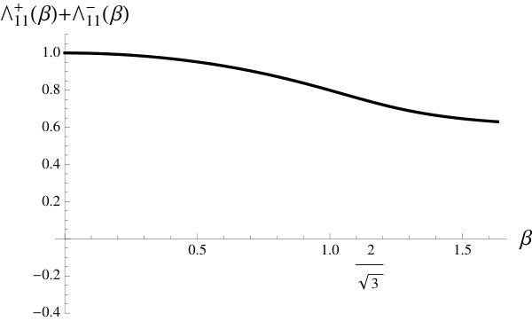 Figure 1
Peer Reviews
No public reviews on file for this paper yet. If you reviewed it on a platform where reviews are public (OpenReview, ICLR, NeurIPS, ICML), you can paste yours below so the community can read it here.
Videos
No videos yet. Explain this paper in a talk, walkthrough, or lecture? Add one.
Inverse Observability Inequalities
for Integrodifferential Equations
in Square Domains
Paola Loreti Dipartimento di Scienze di Base e Applicate per l’Ingegneria Sapienza Università di Roma, Via Antonio Scarpa 16, 00161 Roma (Italy); e-mail: [email protected]
Daniela Sforza Dipartimento di Scienze di Base e Applicate per l’Ingegneria, Sapienza Università di Roma, Via Antonio Scarpa 16, 00161 Roma (Italy); e-mail: [email protected]
Abstract
In this paper we will consider oscillations of square viscoelastic membranes by adding to the wave equation another term, which takes into account the memory. To this end, we will study a class of integrodifferential equations in square domains. By using accurate estimates of the spectral properties of the integrodifferential operator, we will prove an inverse observability inequality.
Keywords: observability; Fourier series; Ingham estimates
MSC: 45K05
1 Introduction
In [11] and [12] we solved a Dirichlet boundary control problem for the wave equation with the exponential memory kernel
[TABLE]
The result was established under some conditions on the parameters and , that is , , . In the investigation a key point to get an estimate for the control time was to prove the inverse inequality. In [12] the analysis was done in the one-dimensional case, obtaining a precise estimate of the observability time . In [13] we also solved the problem for -dimensional balls. It was an open problem to extend to simple domains like rectangles, common in applications, the previous results using the Fourier method. The inverse observability estimate for the wave equation without memory was obtained under the geometrical condition that the control time is greater than twice the diagonal of the rectangle, see [1]. By means of the Fourier method, Mehernberger [14] obtained a weaker result, nevertheless his method can be adapted to get the inverse inequality for other models. See also [7] for an improvement of [14] and further applications.
For another approach we have to mention the paper [5], where the analysis of the kernel is done by a compact perturbation and the author proves his result by means of a unique continuation property of the integro-differential equation. The method proposed by us is more direct and may be easily adapted to other boundary conditions, since in our estimates the dependence on the eigenvalues of the integro-differential operator is explicitly given. Moreover, Theorem 1.3 below has an interest in itself, because it contains a method which is more general than those used in [14, 7].
It is noteworthy that exponential kernels arise in viscoelasticity theory, such as in the analysis of Maxwell fluids or Poynting -Thomson solids, see e.g. [15, 17]. For other references in viscoelasticity theory see the seminal papers of Dafermos [2, 3] and [16, 9].
In this paper we will consider oscillations of square viscoelastic membranes by adding to the wave equation another term, which takes into account the memory. We will fix to study the integrodifferential equation in a square. This assumption has the double target to simplify the computation for the square and to extend to the -d case the results given in [12].
We will go back to the assumption and observe that the estimates we need, still hold in the limiting case . The analysis will require accurate estimates of the asymptotic behavior of the eigenvalues in the complex plane, with precise estimates for the limiting case.
We will consider the following Cauchy problem in the square domain
[TABLE]
In [12] we provided a detailed analysis of the cubic equation associated with the integrodifferential equation. In particular, we gave the asymptotic behavior of the solutions of the cubic equation. Using those results, it is possible to write the solutions of the cubic equation in a different form with respect to that given in [12], but more fitting for the goal of the present paper. Indeed, the following representation for the solution of problem (1) holds.
Theorem 1.1
For any and the weak solution of problem (1) is given by
[TABLE]
with
[TABLE]
where
[TABLE]
Moreover,
[TABLE]
and there exist such that
[TABLE]
Remark 1.2
In formula (2) the coefficients and are uniquely determined by the initial conditions and . Since for our purposes it is only significant the relation (6) between and , we omit the explicit expression of .
In virtue of Theorem 1.1 we are able to establish the following observability estimate on the subset of the boundary of the square domain.
Theorem 1.3
Let . If is the weak solution of problem (1) and , then there exist and such that for all and the inverse observability inequality
[TABLE]
holds true for some positive constant .
We will prove Theorem 1.3 in Section 3.2 after some preliminary results.
2 Estimates of the eigenvalues
In this section we will study the distribution of the eigenvalues in the complex plane. Indeed, using the precise expressions of the eigenvalues provided by Theorem 1.1, we will analyze the behavior of partial gaps helpful to get the observability estimates.
To carry out our analysis, we need also the following known result, see [8].
Lemma 2.1
Fix an integer and integers . If are two positive integers satisfying
[TABLE]
then
[TABLE]
In particular, if one has .
Using the notations introduced in Theorem 1.1 we will prove
Proposition 2.2
If and \beta\in\big{[}0,\frac{2}{\sqrt{3}}\big{]}, there exists such that
[TABLE]
[TABLE]
Moreover, the constant in the previous inequalities can be taken equal to
[TABLE]
In addition
[TABLE]
Proof. First, by taking in formulas (3) and (4), we obtain
[TABLE]
where
[TABLE]
[TABLE]
[TABLE]
Fixed and with , thanks to (12) we have
[TABLE]
We will show that the quantity , regarded as function of , is decreasing for \beta\in\big{[}0,\frac{2}{\sqrt{3}}\big{]}. To do that, in view of (14) and (15) we introduce the functions
[TABLE]
since
[TABLE]
We will prove that is decreasing in \big{[}0,\sqrt{\frac{3}{2}}\big{]}, that is for any x\in\big{[}0,\sqrt{\frac{3}{2}}\big{]}. First, we note that
[TABLE]
Set , in view of
[TABLE]
we can write
[TABLE]
Therefore, is equivalent to
[TABLE]
[TABLE]
and the last inequality is true for and , that is x\in\big{[}0,\sqrt{\frac{3}{2}}\big{]}. Therefore, it remains to be seen
[TABLE]
To this end, taking into account (17), we note that if . Because of we have that for .
Since for \beta\in\big{[}0,\frac{2}{\sqrt{3}}\big{]} we have
[TABLE]
thanks to (18) we can deduce that
[TABLE]
and hence, from (16) it follows
[TABLE]
Moreover, we also note that, thanks to , we have for any , whence we get .
Therefore from (22), using Lemma 2.1, we get
[TABLE]
so, we have shown the first inequality in (8) with \gamma=(\sqrt{2}-1)\big{(}\Lambda^{+}_{11}(\beta)+\Lambda^{-}_{11}(\beta)\big{)}, the same positive constant as in (10). In a similar way one can prove the other inequality in (8).
Finally, in virtue of (12) and (21) we obtain
[TABLE]
that is (9).
Regarding the last statement (11), first we note that follows from (5) since . To prove , we have to take in (3) and show
[TABLE]
that is
[TABLE]
where and are given by (14) and (15) respectively. We observe that
[TABLE]
In virtue of (18), (19) and (20) we have
[TABLE]
Therefore, from (24) we get
[TABLE]
whence, taking also into account (13), we have
[TABLE]
that is (23) holds true.
Remark 2.3
We observe that if we pass to the limit in (10) as , we obtain , that is the value of the gap in the case of classical wave equations in a square domain, see Lemma 2.1.
3 The observability estimate
3.1 The weight function
To prove our results we need to introduce the function
[TABLE]
To begin with, we list some properties of in the following lemma.
Lemma 3.1
Set
[TABLE]
the following properties hold for any
[TABLE]
[TABLE]
[TABLE]
For , and , , we have
[TABLE]
Proof. We have to prove only the last statement. To this end, we observe that
[TABLE]
Since and , we have
[TABLE]
and hence (29) follows.
Theorem 3.2
Assume that there exist and such that
[TABLE]
*and *
[TABLE]
[TABLE]
[TABLE]
Then
[TABLE]
where .
Proof. Set
[TABLE]
we note that
[TABLE]
Let be the function defined by (25). We have
[TABLE]
Since we can get rid of the last term on the right-hand side of the above formula, so we get
[TABLE]
For we have
[TABLE]
so, by applying (27) we obtain
[TABLE]
Similarly, by using again (27) we get
[TABLE]
By putting (36) and (37) into (35), we have
[TABLE]
We may write the first sum on the right-hand side as follows
[TABLE]
Plugging the above identity into (38) we have
[TABLE]
By using the elementary estimate , , we obtain
[TABLE]
By (28) we have and hence
[TABLE]
Similarly
[TABLE]
Moreover,
[TABLE]
Therefore, plugging formulas (40)–(42) into (39) we have
[TABLE]
First, thanks to (26) we note that
[TABLE]
so we can write
[TABLE]
Now, for any we have to estimate the sum
[TABLE]
Since , thanks to assumptions (30) and (31) we can apply (29) to get
[TABLE]
Since we have
[TABLE]
In view of the above estimate, we can write (43) in the following way
[TABLE]
Concerning the third sum on the right-hand side of the previous estimate, as above we can show that
[TABLE]
and hence
[TABLE]
Therefore, from (44) it follows
[TABLE]
Now, we have to estimate the last sum on the right-hand side. Thanks to (33), we have
[TABLE]
Since , again by (29) we have
[TABLE]
As a consequence, we get
[TABLE]
[TABLE]
Plugging the two previous estimates into (46), we obtain
[TABLE]
In addition, keeping in mind also (32), in a similar way it follows
[TABLE]
and hence, by summing the previous two inequalities yields
[TABLE]
where . Finally, putting the previous formula in (45), we get the estimate
[TABLE]
whence, in virtue of the definition of , we obtain (34)
3.2 Proof of Theorem 1.3
Thanks to Theorem 1.1 the weak solution of problem (1) is given by
[TABLE]
Let . We have
[TABLE]
By Proposition 2.2 for any fixed the assumptions of Theorem 3.2 are satisfied with , so applying formula (34) we get
[TABLE]
where . The above formula can be also written in the following way
[TABLE]
Now, we note that in the previous estimate we may change into . Indeed, if we have , while for any we have . So, thanks also to (11), we obtain
[TABLE]
Therefore, in view of (47) it follows
[TABLE]
In a similar way we can establish the following estimate for :
[TABLE]
Thanks to the expression (10) of , there exists such that for any , and hence, for we get
[TABLE]
Therefore, from the previous estimates we can deduce
[TABLE]
By summing (48) and (49) and taking into account that we get
[TABLE]
Finally, again in view of (10), we can pick out sufficiently small such that for any , and hence
[TABLE]
so (7) holds true.
The reference list from the paper itself. Each links out to its DOI / PubMed record.
- 1[1] C. Bardos, G. Lebeau, J. Rauch, Sharp sufficient conditions for the observation, control and stabilization of waves from the boundary , SIAM J. Control Optim. 30 (1992), 1024–1065.
- 2[2] C. M. Dafermos, Asymptotic stability in viscoelasticity , Arch. Rational Mech. Anal., 37 (1970), 297–308.
- 3[3] C. M. Dafermos, An abstract Volterra equation with applications to linear viscoelasticity , J. Differential Equations, 7 (1970), 554–569.
- 4[4] A. E. Ingham, Some trigonometrical inequalities with applications to the theory of series. Math. Z. 41 (1936), 367–379.
- 5[5] J. U. Kim, Control of a second-order integro-differential equation , SIAM J. Control Optim., 31 (1993), 101–110.
- 6[6] V. Komornik, P. Loreti, Fourier Series in Control Theory , Springer-Verlag, New York, 2005.
- 7[7] V. Komornik, P. Loreti, Observability of rectangular membranes and plates on small sets , Evol. Equations and Control Theory 3 (2014), 2, 287–304.
- 8[8] V. Komornik, P. Loreti, Observability of square membranes by Fourier series methods , Bulletin SUSU MMCS 8 (2015), 127-140.