This paper investigates the scaling limits of random plane forests with fixed degree sequences, demonstrating convergence to a continuum random tree in the Gromov-Hausdorff-Prokhorov topology, extending Aldous's framework.
Contribution
It establishes the Gromov-Hausdorff-Prokhorov convergence of large random forests with prescribed degrees to a continuum limit, using excursions of first passage bridges.
Findings
01
Convergence of random forests to Brownian Continuum Random Tree
02
Identification of the limit as a sequence of real trees encoded by excursions
03
Utilization of Lukasiewicz walks to study scaling limits
Abstract
In this paper, we consider the random plane forest uniformly drawn from all possible plane forests with a given degree sequence. Under suitable conditions on the degree sequences, we consider the limit of a sequence of such forests with the number of vertices tends to infinity in terms of Gromov-Hausdorff-Prokhorov topology. This work falls into the general framework of showing convergence of random combinatorial structures to certain Gromov-Hausdorff scaling limits, described in terms of the Brownian Continuum Random Tree, pioneered by the work of Aldous. In fact we identify the limiting random object as a sequence of random real trees encoded by excursions of some first passage bridges reflected at minimum. We establish such convergence by studying the associated Lukasiewicz walk of the degree sequences. In particular, our work is closely related to and uses the results from the…
No public reviews on file for this paper yet. If you reviewed it on a platform where reviews are public (OpenReview, ICLR, NeurIPS, ICML), you can paste yours below so the community can read it here.
Videos
No videos yet. Explain this paper in a talk, walkthrough, or lecture? Add one.
Full text
Scaling limit of random forests with prescribed degree sequences
Tao Lei
Department of Mathematics and Statistics, McGill University, 805 Sherbrooke Street West,
Montréal, Québec, H3A 0B9, Canada
In this paper, we consider the random plane forest uniformly drawn from all possible plane forests with a given degree sequence. Under suitable conditions on the degree sequences, we consider the limit of a sequence of such forests with the number of vertices tends to infinity in terms of Gromov-Hausdorff-Prokhorov topology. This work falls into the general framework of showing convergence of random combinatorial structures to certain Gromov-Hausdorff scaling limits, described in terms of the Brownian Continuum Random Tree (BCRT), pioneered by the work of Aldous [6, 7, 8]. In fact we identify the limiting random object as a sequence of random real trees encoded by excursions of some first passage bridges reflected at minimum. We establish such convergence by studying the associated Lukasiewicz walk of the degree sequences. In particular, our work is closely related to and uses the results from the recent work of Broutin and Marckert [16] on scaling limit of random trees with prescribed degree sequences, and the work of Addario-Berry [3] on tail bounds of the height of a random tree with prescribed degree sequence.
2010 Mathematics Subject Classification:
60C05
1. Introduction
Scaling limits for finite graphs is a topic at the intersection of combinatorics and probability. In this paper, we investigate the Gromov-Hausdorff-Prokhorov convergence of random forests with prescribed degree sequence. Our work is a natural continuation of [16] where it is shown that under natural hypotheses on the degree sequences, after suitable normalization, uniformly random trees with given degree sequence converge to Brownian continuum random tree, with the size of trees going to infinity.
In a series of papers [6, 7, 8], Aldous introduced the concept of Brownian continuum random tree (BCRT) and showed that critical Galton-Watson tree conditioned on its size has BCRT as limiting objects. Since then, many families of graphs have been shown to have BCRT or random processes derived from BCRT as their limiting objects. For example, multi-type Galton-Watson trees [26], unordered binary trees [24], critical Erdös-Rényi random graph [4], random planar maps with a unique large face [22], random planar quadrangulations with a boundary [13].
As in [16], our combinatorial model is motivated by the metric structure of graphs with a prescribed degree sequence. This model was first introduced by Bender and Canfield [11] and by Bollobás [15] in the form of the configuration model. This model can give rise to graphs with any particular (legitimate) prescribed degree sequence (including, e.g., heavy tailed degree distributions, a feature which is observed in realistic networks but is not captured by the Erdös-Rényi random graph model).
Our main results, which are stated formally in Section 1.2, are that, under natural assumptions on degree sequences and after suitable normalization, large uniformly random forests with given degree sequence converge in distribution to the forests coded by Brownian first passage bridge, with respect to the Gromov-Hausdorff-Prokhorov topology. In order to present these results rigorously, we need the following subsection to introduce the necessary concepts and notations involved.
1.1. Definitions and Notation
Plane trees and forests
We recall the following definition of plane trees (as in e.g. [19]). Let
[TABLE]
where N={1,2,⋯} and N0={∅}. If u=(u1,u2,⋯,un)∈U we write u=u1u2⋯un for short and let ∣u∣=n be the generation of u. If u=u1⋯um,v=v1⋯vn, we write uv=u1⋯umv1⋯vn for the concatenation of u and v.
Definition 1.1**.**
A rooted plane tree T is a subset of U satisfying the following conditions:
(i) ∅∈T;
(ii) If v∈T and v=uj for some u∈U and j∈N, then u∈T;
(iii) For every u∈T, there exists a number kT(u)≥0 such that uj∈T if and only if 1≤j≤kT(u). We call kT(u) the degree of u in T.
We denote the lexicographic order on U by < (e.g. ∅<11<21<22). The lexicographic order on U induces a total order on the set of all rooted plane trees.
We call a finite sequence of finite rooted plane trees F=(T1,T2,⋯,Tm) a rooted plane forest. For forest F, we let F↓ be the sequence of tree components of F in decreasing order of size, breaking ties lexicographically (if again tied, then as the original order of appearance in F).
Definition 1.2**.**
A degree sequence is a sequence s=(s(i),i≥0) of non-negative integers with i≥0∑s(i)<∞ such that c(s):=i≥0∑(1−i)s(i)>0.
For a plane tree T, the degree sequence s(T)=(s(i)(T),i≥0) is given by
[TABLE]
For a plane forest F=(T1,⋯,Tm), the degree sequence s(F)=(s(i)(F),i≥0) is given by
[TABLE]
Note that c(s(T))=1 for any plane tree T. In general since
[TABLE]
and i≥0∑s(i)(F)=j=1∑m∣Tj∣, the number of tree components in F is always c(s(F)). For any degree sequence s, we adopt the notations
[TABLE]
Figure 1, below, shows a plane forest with degree sequence s=(7,2,2,1,0,⋯) with s(i)=0 for i≥4.
For any degree sequence s=(s(i),i≥0), we let F(s) denote the set of all plane forests with degree sequence s. Let Ps be the uniform measure on F(s) and let F(s) be a random plane forest with law Ps.
First passage bridge
We also need to recall the following definition of first passage bridge as in [10]. Informally, for λ>0, the first passage bridge of unit length from 0 to −λ, denoted Fλbr, is a C[0,1]−valued random variable with law
[TABLE]
where B is a standard Brownian motion and Tλ:=inf{t:B(t)<−λ} is the first passage time below level −λ<0.
For l≥0, we write Blbr for the Brownian bridge of duration 1 from 0 to −l. As explained in Proposition 1 of [21], the law of the
Brownian bridge Blbr is characterized by Blbr(1)=−l and the formula
[TABLE]
for all bounded measurable function f, and all 0≤m<1, where pa is the Gaussian density with variance a and mean 0, that is, pa(x)=2πa1e−2ax2.
In a similar way the law of Fλbr can be defined as the law such that
[TABLE]
for all bounded measurable functions f and all 0≤s<1 and Fλbr(1)=−λ, where pa′ is the derivative of pa. These formulae set the finite-dimensional laws of the first passage bridge. In [12] (see Section 5.1 for details) it is shown that it admits a continuous version, and that Fλbr is the weak limit of Fλϵ where (Fλϵ(t),0≤t≤1) has the law of B conditioned on the event {B(1)<−λ+ϵ,s≤1infB(s)>−λ−ϵ}, hence justifying the informal conditioning definition.
Gromov-Hausdorff-Prokhorov distance
We recall the definition of the Gromov-Hausdorff distance (see for example Definition 7.3.10 in [17]). Let (X,d) and (X′,d′) be compact metric spaces. Then the Gromov-Hausdorff distance between (X,d) and (X′,d′) is given by
[TABLE]
where the infimum is taken over all isometric embeddings ϕ:X↪Z and ϕ′:X′↪Z into some common Polish metric space (Z,dZ) and dHZ denotes the Hausdorff distance between compact subsets of Z, that is,
[TABLE]
where Aϵ is the ϵ−enlargement of A:
[TABLE]
Note that strictly speaking dGH is not a distance since different compact metric spaces can have GH distance zero.
A rooted measured metric spaceX=(X,d,∅,μ) is a metric space (X,d) with a distinguished element ∅∈X and a finite Borel measure μ. Note that the definitions in this subsection work in more general settings, e.g. μ could be a boundedly finite Borel measure (see [2]), but for the purpose of this paper, finite measure μ is enough.
Let X=(X,d,∅,μ) and
X′=(X′,d′,∅′,μ′) be two compact rooted measured metric spaces, they are GHP-isometric if there exists an isometric one-to-one map Φ:X→X′ such that Φ(∅)=∅′ and Φ∗μ=μ′ where Φ∗μ is the push forward of measure μ to (X′,d′), that is, Φ∗μ(A)=μ(Φ−1(A)) for A∈B(X′). In this case, call Φ a GHP-isometry.
Suppose both X and X′ are compact, then define the Gromov-Hausdorff-Prokhorov distance as:
[TABLE]
where the infimum is taken over all isometric embeddings Φ:X↪Z and Φ′:X′↪Z into some common Polish metric space (Z,dZ), and dPZ denotes the Prokhorov distance between finite Borel measures on Z, that is,
[TABLE]
Let K denote the set of GHP-isometry classes of compact rooted measured metric spaces and we identify X with its GHP-isometry class. We have the following results from [2]:
The function dGHP defines a metric on K and the space (K,dGHP) is a Polish metric space.
We next define a distance between sequences of rooted measured metric spaces. For X=(Xj,j≥1),X′=(Xj′,j≥1) in KN, we let
[TABLE]
If X∈Kn for some n∈N, in order to view X as a member of KN, we append to X an infinite sequence of zero metric spaces Z. Here Z is the rooted measured metric space consisting of a single point with measure 0. Let Z=(Z,Z,⋯) and
[TABLE]
By definition of GHP distance it is not hard to see that dGHP(X,Z)=2diam(X)+μ(X), hence X∈L∞ if and only if j→∞limsup(diam(Xj)+μj(Xj))=0. It is likewise straightforward to show that (L∞,dGHP∞) is a complete separable metric space.
Real trees
Next we briefly recall the concepts of real trees and real trees coded by continuous functions. A more lengthy presentation about the probabilistic aspects of real trees can be found in [20, 23].
Definition 1.4**.**
A compact metric space (T,d) is a real tree if the following hold for every a,b∈T:
(i) There is a unique isometric map fa,b from [0,d(a,b)] into T such that fa,b(0)=a and fa,b(d(a,b))=b.
(ii) If q is a continuous injective map from [0,1] into T, such that q(0)=a and q(1)=b, we have q([0,1])=fa,b([0,d(a,b)]).
A real tree (T,d) is rooted if there is a distinguished vertex (the root) ∅∈T and we denote a rooted real tree by (T,d,∅). If there is a finite Borel measure μ on T, then (T,d,∅,μ) is a measured rooted real tree.
Next we show a way of constructing real trees from continuous functions. Let g:[0,∞)→[0,∞) be a continuous function with compact support and such that g(0)=0. For every s,t≥0, let
[TABLE]
where
[TABLE]
The function dg∘ is a pseudometric on [0,∞). Define an equivalence relation ∼ on [0,∞) by setting s∼t iff dg∘(s,t)=0. Then let Tg=[0,∞)/∼ and let dg be the induced distance on Tg. Then (Tg,dg) is a real tree (see, e.g. Theorem 2.2 in [23]).
To get an intuition of this construction, for a rooted plane tree T with graph distance dgr, let T^ be the metric space obtained from T by viewing each edge as an isometric copy of the unit interval [0,1], and imagine a particle exploring the tree, starting from the root and moving at unit speed. Each time the particle leaves a vertex u, it moves to the lexicographically next unvisited child of u, if such a child exists; otherwise it moves to the parent of u. The exploration concludes the moment the particle has visited all vertices and returned to the root. Let C:[0,2(∣T∣−1)]→[0,∞) be such that C(t) equals to the graph distance between the particle and the root at time t. C is called the contour function of T. Then the metric space TC constructed from C is isometric to T^.
Let ∅g denote the equivalence class of 0. Let pg be the canonical projection from [0,∞) to Tg and σg=sup{t:g(t)>0}. Let mg be the push forward of the Lebesgue measure on [0,σg] ((σg,∞) has measure 0) by pg. Then Tg=(Tg,dg,∅g,mg) is a compact measured rooted real tree. In particular, Tg∈K. Let e denote the standard Brownian excursion, then Te is called the Brownian continuum random tree (BCRT for short).
1.2. Statement of main theorems
For c>0, let ce∈C[0,∞) denote the Brownian excursion of length c, that is (ce)(s):=ce(cs∧1) for s≥0. For any probability distribution p=(p(i),i≥0) on N, let μ(p)=i≥0∑ip(i) and σ2(p)=i≥0∑i2p(i).
In this paper we consider a sequence of degree sequences (sκ,κ∈N), where sκ=(sκ(i),i≥0). We assume nκ:=i≥0∑sκ(i)→∞ and let Fκ:=F(sκ) and write Fκ↓=(Tκ,l,l≥1). We write pκ=(pκ(i),i≥0):=(nκsκ(i),i≥0). For Fκ↓=(Tκ,l,l≥1), let Tκ,l denote the measured rooted real tree (Tκ,l,2nκ1/2σκdgr,∅κ,l,μκ,l) where σκ=σ(pκ) and μκ,l denotes the uniform measure putting mass nκ1 on each vertex of Tκ,l. Let Fκ↓=(Tκ,l,l≥1). Let Δκ:=max{i:sκ(i)>0}. We are now prepared to state our main theorems.
Theorem 1.5**.**
Suppose that there exists a distribution p=(p(i),i≥0) on N with p(1)<1 such that pκ converges to p coordinatewise. Suppose also that σ(pκ)→σ(p)∈(0,∞). If σ(pκ)nκ1/2c(sκ)→λ∈(0,∞), then
[TABLE]
with respect to the product topology for dGHP where (γl,l≥1) are the excursions of the process (Fλ(s)−s′∈(0,s)infFλ(s′))0≤s≤1, listed in decreasing order of length.
Theorem 1.6**.**
Under the conditions of Theorem 1.5, suppose additionally that there exists ϵ>0 such that Δκ=O(nκ21−ϵ). Then the convergence (1.3) holds in (L∞,dGHP∞).
Remark 1.1**.**
The assumptions of Theorem 1.5 imply that μ(pκ)→μ(p)=1 and that Δκ=o(nκ1/2). We include the proof of these facts as Lemma A.1 in the Appendix.
Remark 1.2**.**
The pair ((γl,l≥1),(Tγl,l≥1)) has the same law as ((γl,l≥1),(T∣γl∣el,l≥1)) where (el,l≥1) are standard Brownian excursions, independent of each other and of (γl,l≥1).
1.3. Key ingredients of the paper
Here we summarize the two key ingredients of this paper. The first element is the convergence of the large trees in (1.3), which is essentially given by the following proposition. For all l≥1, let Xκ,l=nκ∣Tκ,l∣.
Proposition 1.7**.**
Under the conditions of Theorem 1.5, for any fixed j≥1,
[TABLE]
as κ→∞, where (el)l≤j are independent copies of e, and (γl,l≥1) are the excursions of (Fλ(s)−s′∈(0,s)infFλ(s′))0≤s≤1 ranked in decreasing order of length.
There are two parts of the convergence in (1.4). One is the convergence of the normalized sizes of large trees to lengths of excursions. This will be given by the following proposition. To state this result, we need to first introduce some notions. Let C0(1)={x∈C([0,1],R):x(0)=0}
For a non-negative function g+∈C0(1), an excursionγ of g+ is the restriction of g+ to a time interval [l(γ),r(γ)] such that g+(l(γ))=g+(r(γ))=0 and g+(s)>0 for s∈(l(γ),r(γ)). In this case [l(γ),r(γ)] is called an excursion interval of g+. The length of the excursion is denoted as ∣γ∣=r(γ)−l(γ). For a function g we write g(s)−0≤s′<sming(s′) to denote (g(s)−0≤s′<sming(s′),0≤s≤1). For g∈C0(1), sometimes we refer the excursions of g(s)−0≤s′<sming(s′) as excursions of g. Let l1↓={x=(x1,x2,⋯):x1≥x2≥⋯≥0,i∑xi≤1} and endow l1↓ with the topology induced by the l1 distance: d(x,y)=i∑∣xi−yi∣.
in l1↓, where (γl,l≥1) are the excursions of Fλbr(s)−0≤s′≤sminFλbr(s′) ranked in decreasing order of length.
This proposition will be a corollary of the following theorem, which is the main result of Section 4. For a plane forest F, let u1<u2<⋯<u∣F∣ be the nodes of F listed according to their lexicographical order in U in each tree component, with nodes of first tree listed first, then the nodes of second tree and so on. The depth-first walk, or Lukasiewicz pathSF is defined as follows. First set SF(0)=0 and then let
[TABLE]
We extend the definition of SF to the compact interval [0,∣F∣] by linear interpolation.
The second part of the convergence of (1.4) is the convergence of the large trees, for which we will rely on the following result about random trees with given degree sequences from [16].
Let {sκ,κ≥1} be a degree sequence such that nκ:=n(sκ)→∞,Δκ:=Δ(sκ)=o(nκ1/2). Suppose that there exists a distribution p on N with mean 1 such that pκ converges to p coordinatewise and such that σ(pκ)→σ(p)∈(0,∞). Let Tκ be the random plane tree under Psκ, the uniform measure on the set of plane trees with degree sequence sκ. Let Tκ denote the measured rooted metric space (Tκ,2nκ1/2σ(pκ)dgr,∅κ,μκ) where μκ denotes the uniform measure putting mass nκ1 on each vertex of Tκ. Then when κ→∞,Tκ→dTe in the Gromov-Hausdorff-Prokhorov sense.
Remark 1.3**.**
In fact Theorem 1 in [16] is only stated in the Gromov-Hausdorff sense, that is, (Tκ,2nκ1/2σ(pκ)dgr)→d(Te,de,∅e). But the conclusion can be strengthened to GHP convergence easily. For completeness, we include a proof of this fact in Appendix B.
The following proposition contains the additional ingredient required to prove Theorem 1.6.
Proposition 1.11**.**
Under the conditions of Theorem 1.6, for all a>0, we have
[TABLE]
The key results leading to Proposition 1.11 include a height bound for random tree with prescribed degree sequence and a variance bound for uniformly permuted child sequences. The height bound of uniformly random tree with prescribed degree sequence is given in the following theorem.
Fix a degree sequence s=(s(i),i≥0) such that i≥0∑is(i)=∣s∣−1, and let T(s) be a uniformly random plane tree with degree sequence s. Then for all m≥1 we have
[TABLE]
where 1s=∣s∣−1−s(1)∣s∣−2.
The following probability bound on variances of uniformly permuted integer sequences allows us to control the variance of degrees of trees in random forests, and thereby apply Theorem 1.12 to prove Proposition 1.11.
Proposition 1.13**.**
Fix c=(c1,⋯,cn)∈Nn and let π be a uniformly random permutation of {1,⋯,n}. Set Ci=cπ(i) for 1≤i≤n, and let Sj=i≤j∑Ci2 for 1≤i≤n. Then for all λ≥2 and 1≤k≤n, with Δ=1≤i≤nmaxCi=1≤i≤nmaxci, and σ2(c)=i≤n∑ci2=Sn, we have
[TABLE]
Now let us prove our main theorems with these key results.
By Skorokhod’s representation theorem, we may work in a probability space in which the convergence in Proposition 1.7 is almost sure. Hence Proposition 1.7 yields that for any fixed j,l≤jsupdGHP(Tκ,l,T∣γl∣el)→d0. This establishes Theorem 1.5.
Now to prove the convergence in (L∞,dGHP∞), it suffices to prove
that for any a>0,
[TABLE]
It suffices to separately prove
[TABLE]
[TABLE]
For this purpose, we need to control the probability that small trees having either large diameter or large mass. Note that for a tree its diameter is bounded by twice of its height.
In fact the mass of tree is easy to control since for any a>0 and any κ,
We also need to bound diam(Tγl) and mass(Tγl) for l large. Note that mass(Tγl)=∣γl∣ and for any a, let j>1/a, then P(l>jsup∣γl∣>a)=0.
For diam(Tγl),diam(Tγl)≤2h(Tγl)=2max(γl). For 0≤s≤1, let
[TABLE]
and the excursion interval of γl be [gl,dl]. Then
[TABLE]
and dl−gl=∣γl∣≤1/l.
So for any j≥1/ϵ,
[TABLE]
since Fλ is uniformly continuous. Hence we have the tail insignificance for diameter of Tγl and the claim is proved.
∎
To conclude this section, we sketch how our paper is organized. In Section 2 we investigate a special rotation mapping, which connects the collection of lattice bridges corresponding to certain degree sequence s and the set of first passage lattice bridges corresponding to s. This will be the key starting point of our work using depth-first walk process to code the structure of random forests with given degree sequences. The combinatorial argument in this section will be also useful for our later work on transferring results such as Proposition 1.13 to something similar which is applicable to random forests. This section will be purely combinatorial and only deal with fixed degree sequences. In Section 3, we collect some concentration results using martingale methods. These probability bounds will be useful for checking that the assumptions in Theorem 1.10 are satisfied for large trees of Fκ↓. The second part of this section proves the variance bound in Proposition 1.13. Again all results in this section is non-asymptotic and hence are presented with regards to a fixed degree sequence. In Section 4, we prove Theorem 1.9, the convergence of scaled exploration processes to some random process related to first passage bridge, using the rotation mapping in Section 2. We will then get Proposition 1.8 as a corollary from this weak convergence result. Finally, in Section 5 we finish the proof of Proposition 1.7 and Proposition 1.11 using results from Section 3 and Section 4.
2. An n−to−1 map transforming lattice bridge to first passage lattice bridge
Given a degree sequence s=(s(i),i≥0), let d(s)∈Z≥0n(s) be the vector whose entries are weakly increasing and with s(i) entries equal to i, for each i≥0. For example, if s=(3,2,0,1,0,⋯) with s(i)=0 for i≥4, then d(s)=(0,0,0,1,1,3). Let D(s) be the collection of all possible child sequences corresponding to degree sequence s, i.e., all possible result as a permutation of d(s).
A lattice bridge is a function b:[0,k]→R with b(0)=0 and b(i)∈Z,∀i∈[k], which is piecewise linear between integers. Here k is an arbitrary positive integer. We let
[TABLE]
and call Λ(s) the set of lattice bridges corresponding to s. Note that if b∈Λ(s), then b(n(s))=−c(s). Furthermore, we have
[TABLE]
since to determine b∈Λ(s), it suffices to choose the s(0) positions with step size −1, s(1) positions with step size 0, s(2) positions with step size 1, etc.
We then let
[TABLE]
and call F(s) the collection of first passage lattice bridges corresponding to s.
For s>0, let C0(s)={x∈C([0,s],R):x(0)=0}. For u∈[0,s], let θu,s:C0(s)→C0(s) denote the cyclic shift at u, that is,
[TABLE]
For x∈C0(s) and y∈R−, let t(y,x):=inf{t∈[0,s]:x(t)≤y} be the first time the graph of x drops below y. Sometimes we drop the argument x for convenience and simply write t(y). If y<u∈[0,s]minx(u) we set t(y,x)=0 by convention, so θt(y)(x)=x.
In what follows, for k∈N we write [k]−1={0,1,⋯,k−1}. And when the context is clear, we simply drop the subscript s and write θu for θu,s.
Lemma 2.1**.**
For b∈Λ(s), and for each j∈[c(s)]−1, we have θt(min(b)+j)(b)∈F(s).
Proof.
Let m≤0 be the minimum of b. Fix an integer i such that m≤i≤m+c(s)−1 and u<n(s). We shall prove that θt(i)(b)(u)>−c(s), which proves the lemma.
If 0≤u≤n(s)−t(i), then θt(i)(b)(u)=b(t(i)+u)−b(t(i))≥m−i>−c(s). If n(s)−t(i)≤u<n(s), then θt(i)(b)(u)=b(t(i)+u−n(s))+b(n(s))−b(t(i))=b(t(i)+u−n(s))−c(s)−i. Since u<n(s), t(i)+u−n(s)<t(i) and we must have b(t(i)+u−n(s))>i by our definition of t. Therefore in this case we also have θt(i)(b)(u)>−c(s).
∎
Next, define a function f:Λ(s)×([c(s)]−1)→F(s) by f(b,j):=θt(min(b)+j)(b).
Lemma 2.2**.**
f* is an n(s)−to−1 map from Λ(s)×([c(s)]−1) to F(s).*
Proof.
For l∈F(s), if size of preimage of l under f is strictly large than n(s), then we must have b1,b2∈Λ(s),j1,j2∈[c(s)]−1 such that f(b1,j1)=f(b2,j2)=l and t(min(b1)+j1)=t(min(b2)+j2), since t can only take values in [n(s)]. By the definition of f we must then have b1=b2 and hence j1=j2. Therefore each element in F(s) can have at most n(s) preimages in Λ(s)×([c(s)]−1). On the other hand, we have (see, e.g., [28], page 128)
[TABLE]
Hence n(s)×∣F(s)∣=c(s)×∣Λ(s)∣=∣Λ(s)×([c(s)]−1)∣, so it must in fact hold that each l∈F(s) has exactly n(s) preimages.
∎
Recall the concept of depth-first walk SF of a plane forest F. For a sequence c=(c1,⋯,cn)∈Rn, we write Wc(j)=i=1∑j(ci−1) for j∈[n]. We let Wc(0)=0 and make Wc a continuous function on [0,n] by linear interpolation. Note that SF is precisely Wc where c=(kF(u1),⋯,kF(u∣F∣)).
For c=(c1,⋯,cn)∈Rn and a permutation π of [n], write π(c)=(cπ(1),⋯,cπ(n)). Also, recall from the beginning of this section that for a degree sequence s, d(s) is a vector with s(i) entries equal to i for each i≥0.
Corollary 2.3**.**
Let s be a degree sequence. Let π be a uniformly random permutation of [n(s)] and let ν be independent of π and drawn uniformly at random from [c(s)]−1. Then
[TABLE]
and both are uniformly random elements of F(s).
Proof.
By definition, (Wπ(d(s)),ν) is uniformly at random in Λ(s)×([c(s)]−1). By Lemma 2.2, it follows that f(Wπ(d(s)),ν) is uniformly random in F(s). On the other hand, the map sending plane forest F to its Lukasiewicz path SF restricts to an invertible map from F(s) to F(s). Thus, SF(s) is also uniformly distributed in F(s).
∎
First-passage bridges are naturally connected to plane forests. In a similar way, general lattice bridges are naturally connected to marked plane forests. This interpretation will be more convenient for some later proofs (Propositions 3.5, 3.9 and 3.10).
A marked forest is a pair (F,v) where F is a plane forest and v∈v(F). Sometimes we refer v as the mark of (F,v).
Recall that F(s) denotes the collection of all plane forests with degree sequence s. Let MF(s) be the collection of all marked forests with degree sequence s and for 1≤i≤c(s), let MFi(s) be the collection of marked forests (F,v)∈MF(s) such that the mark v lies within the i−th tree of F. We define a map g:MF(s)→D(s) which lists the degrees of vertices of a marked forest starting from the mark in DFS order. Formally, for (F,v)∈MF(s), if the DFS ordering of v(F) is v1,⋯,vn(s) and v=vi, then g((F,v))=(kF(vi),⋯,kF(vn(s)),kF(v1),⋯,kF(vi−1)). Next define a map h:MF(s)→F(s) by h((F,v))=F. Then we have the following easy fact.
Lemma 2.4**.**
g* is a c(s)−to−1 surjective map and for each 1≤i≤c(s),gi:=g∣MFi(s) is a bijection between MFi(s) and D(s). Also, h is a n(s)−to−1 surjective map.*
Proof.
For d∈D(s),∣g−1({d})∩MFi(s)∣=1 for all 1≤i≤c(s). In fact, the element of each g−1({d})∩MFi(s) can be obtained by cyclically permuting the tree components of the element of g−1({d})∩MF1(s). This shows that gi is a bijection. The other two claims are straightforward.
∎
The map g being surjective immediately gives the following result.
Corollary 2.5**.**
*Let MF(s) be a uniformly random element of MF(s), then g(MF(s)) is a uniformly random element of D(s).
*
3. Concentration results
In the first part of this section, we deal with a martingale concerning the proportion of a fixed degree of uniformly permuted degree sequence. This will be useful for proving Proposition 1.7 in Section 5 where we need to first show that the degree proportions in each large trees of Fκ↓ are more or less in line with the degree proportion of the given degree sequences. The second part of this section deals with the variance bound of uniformly permuted child sequences, which leads to a key technical proposition on the height of tree components of F(s). For both subsections we will use concentration results from [25].
Let s=(s(i),i≥0) with ∣s∣=n be a fixed degree sequence and let C=(C1,⋯,Cn) denote the uniformly permuted child sequence π(d(s)) (recall the notation from Section 2), where π is a uniform random permutation of [n]. For each i≥0, let q(i)=s(i)/n be the degree proportion of degree i of s.
3.1. Martingales of degree proportions of uniformly permuted degree sequence
In this subsection, we introduce some martingales concerning proportions of particular degree appeared at each step in a uniformly permuted degree sequence and use them and martingale concentration inequality from [25] as tools to prove Lemma 3.4 and Proposition 3.5, which are useful for eventually proving that the empirical degree distributions of large trees of Fκ behave well (Proposition 5.1).
We first recall the following martingale bound in [25]. Let {Xi}i=0n be a bounded martingale adapted to a filtration {Fi}i=0n. Let V=i=0∑n−1var{Xi+1∣Fi}, where
Fix s<n, and consider the martingale {Mj(i)}j=0n−s. By Lemma 3.2(b), we know that
[TABLE]
Hence v=\mboxesssupV≤2s1. Also, for j≤n−s−1, if Xj+1(i)=Xj(i), then
[TABLE]
and if Xj+1(i)=Xj(i)−1, then
[TABLE]
Applying Theorem 3.1 to both {Mj(i)}j=0n−s and {−Mj(i)}j=0n−s gives
[TABLE]
as claimed.
∎
Now we give a probability bound of proportion of certain degree i deviates from q(i) by an error of at least ϵ.
Lemma 3.4**.**
For fixed i∈N and ϵ>0, let Bϵ,i={∃x≥log3n:∣Yx(i)−q(i)x∣≥ϵx}.
Then for any n large enough such that logn5<ϵ<1,P(Bϵ,i)≤n−3.
Proof.
By symmetry, the event {∃j≥log3n:∣Yj(i)−q(i)j∣≥ϵj} has the same distribution as the event {∃l≤n−log3n:∣Xl(i)−q(i)(n−l)∣≥ϵ(n−l)}. Hence we can write
[TABLE]
Taking s=log3n,t=ϵ in (3.1), the result follows.
∎
Now we consider how degrees distribute among the tree components of the random forest F(s).
Write F(s)↓=(Tl,l≥1). Let sl=(sl(i),i≥0) denote the (empirical) degree sequence of the l−th largest tree Tl, and let nl=n(sl). Recall that q(i)=s(i)/n and let ql(i)=sl(i)/nl be the empirical proportion of degree i vertices of Tl; if F(s) has fewer than l trees then ql(i)=0. Note that q(i) is deterministic while ql(i) is random.
Proposition 3.5**.**
For fixed ϵ>0 and i,l, let Blϵ,i={∣ql(i)−q(i)∣>ϵ}. Then for fixed ϵ>0,i∈N, we have
[TABLE]
Proof.
Let V be a uniformly random vertex of F(s), then (F(s),V) is uniformly distributed in MF(s). List the nodes of F(s) in cyclic lexicographic order as V=V1,V2,⋯,Vn, and for i≤n let Ci be the degree of Vi. By Corollary 2.5, the sequence (C1,⋯,Cn)=g(F(s),V) is uniformly distributed in D(s); in other words, it is distributed as a uniformly random permutation of d(s). For any 1≤j≤n, let B~jϵ,i be the event that there exists m>n1/4 such that
[TABLE]
Since (C1,⋯,Cn) is uniformly distributed in D(s), it is immediate that P(B~1ϵ,i)=⋯=P(B~nϵ,i). Suppose a tree T∈F(s) with ∣T∣>n1/4 has that
[TABLE]
If V is not a node of T, then there exists m>n1/4,0<j≤n−m such that
[TABLE]
If V is a node of T, then there exists m>n1/4,j>n−m such that
[TABLE]
In either case we must have B~jϵ,i true for some 1≤j≤n. Therefore
[TABLE]
which gives the claim.
∎
3.2. Probability bound of trees of random forest having abnormally large height
In this subsection, we prove tail bounds on the heights of trees in F(s), by first proving tail bounds on the sums of squares of the child sequences. This will be used in proving Proposition 1.11 in Section 5. To be more specific, let c=(c1,c2,⋯,cn)∈D(s) be a child sequence with σ2(s):=i=1∑nci2=i∑i2s(i) and write M:=σ2(s)/n and Δ=Δ(s):=imaxci. Recall that C1,C2,⋯,Cn are the uniformly permuted child sequence and let Sj:=i≤j∑Ci2.
We will use the following theorem from [25].
Let random variables X1∗,⋯,Xn∗ be independent, with Xk∗−E[Xk∗]≤b for each k. Let Sn∗=∑Xk∗, and let Sn∗ have expected value μ and variance V (the sum of the variances of Xk∗). Then for any t≥0, with ϵ=bt/V, we have
[TABLE]
Since C1,C2,⋯,Ck are sampled without replacement from the population c1,c2,⋯,cn, we may not directly apply Theorem 3.6. We address this issue as follows.
Recall (or see, e.g., [5]) that given real random variables U,V, we say U is a dilation of V if there exist random variables U^,V^ such that
Suppose X1,⋯,Xk and X1∗,⋯,Xk∗ are samples from the same finite population x1,⋯,xn, without replacement and with replacement, respectively. Let Sk=i=1∑kXi,Sk∗=i=1∑kXi∗. Then Sk∗ is a dilation of Sk. In particular, E[ϕ(Sk∗)]≥E[ϕ(Sk)] for all continuous convex function ϕ:R→R.
The proof of Theorem 3.6, in [25], proceeds by bounding the quantity E[exp(h(Sn∗−μ))], where h is any real number. By Proposition 3.7, we have E[exp(h(Sn−μ))]≤E[exp(h(Sn∗−μ)], which means that the proof applies mutatis mutandis in the setting of sampling without replacement.
Corollary 3.8**.**
Let X1,⋯,Xk be samples from finite population x1,⋯,xn, without replacement, with X1−E[X1]≤b. Let Sk=i=1∑kXi,V=i=1∑kVar(Xi) and μk=E[Sk]. Then for any t≥0, with ϵ=bt/V, we have
[TABLE]
Now we get our probability bound on the deviations of (Sk,k≤n).
where M=σ2(c)/n. For λ>1, taking t=(λ−1)nkσ2(c), we obtain
[TABLE]
Using the assumption λ≥2 twice, we have
[TABLE]
which finishes the proof.
∎
Using results from Section 2, we now have the following estimate on variance of tree components of F(s).
For a tree T, we let σ2(T)=u∈T∑kT(u)2.
Proposition 3.9**.**
Let s=(s(i),i≥0) be a degree sequence with ∣s∣=n and M=σ2(s)/n. Then for λ≥4,α>Δ2(s)/n,
[TABLE]
Proof.
Let V be a uniformly random vertex of F(s), then (F(s),V) is uniformly distributed in MF(s). List the nodes of F(s) in cyclic lexicographic order as V=V1,V2,⋯,Vn, and for i≤n let Ci be the degree of Vi. By Corollary 2.5, the sequence (C1,⋯,Cn)=g(F(s),V) is uniformly distributed in D(s); in other words, it is distributed as a uniformly random permutation of d(s). In what follows we omit some floor notations for readability. For 0≤j≤⌊α1⌋, let Bj be the event that
[TABLE]
Since C1,⋯,Cn is distributed as a uniformly random permutation of d(s), we clearly have
[TABLE]
Suppose that a given tree T∈F(s) has ∣T∣≤αn and σ2(T)≥λασ2(s). Then there exist 0≤l<n and m≤αn such that V(T)={Vl+t(modn):1≤t≤m}. Hence there exists 0≤j≤⌊α1⌋ such that V(T)⊂{Vi(modn),jαn+1≤i≤(j+2)αn}. This implies that
[TABLE]
i.e. Bj is true. Hence the probability in question is at most
[TABLE]
where we take k=⌊2αn⌋ in Proposition 1.13 and use α>Δ2(s)/n at the last step.
∎
Now we finish this section by proving a key proposition on probability bound of F(s) containing trees with unusually large height.
Proposition 3.10**.**
∀ϵ,ρ∈(0,1),∃n0=n0(ϵ)∈N* and β0>0 such that the following is true. Let s be any degree sequence with ∣s∣=n≥n0. Suppose that Δ(s)≤n21−ϵ,s(1)≤(1−ϵ)∣s∣ and ϵ≤σ2(s)/n≤1/ϵ, then for any 0<β<β0,*
[TABLE]
Proof.
Fix β>0 small, let δ=β1/8, and consider the following four events.
•
E1 is the event that there exists a tree T (of F(s)) with Δ2(s)<∣T∣<βn and σ2(T)>(n∣T∣)1/2σ2(s).
•
E2 is the event that there exists a tree T with ∣T∣≤n1−ϵ and σ2(T)>n1−2ϵ.
•
E3 is the event that there exists a tree T with Δ2(s)<∣T∣<βn and σ2(T)≤(n∣T∣)1/2σ2(s) such that h(T)>δn1/2.
•
E4 is the event that there exists a tree T with ∣T∣≤n1−ϵ and σ2(T)≤n1−2ϵ such that h(T)>δn1/2.
If there is T∈F(s) with ∣T∣<βn, and h(T)>δn1/2, then one of E1,E2,E3 or E4 must occur, so it suffices to bound P(E1)+P(E2)+P(E3)+P(E4).
For E1, we further decompose the interval [Δ2(s),βn] dyadically. In the next sum, we bound the k−th summand by taking α=2kβ,λ=β1/222k−1≥4 in Proposition 3.9.
[TABLE]
where we use that σ2(s)/n≥ϵ in the final line.
Next, note that
P(E2)≤j=1∑n1−ϵP(∃T∈F(s):∣T∣=j,σ2(T)>n1−ϵ/2).
For any fixed j, using Corollary 2.5, with similar argument as in proof of Proposition 3.9, we have
[TABLE]
For any j≤n1−ϵ, use Proposition 1.13 with λnjσ2(s)=n1−ϵ/2 and Δ(s)≤n21−ϵ, we have
[TABLE]
These give that
[TABLE]
We bound P(E3) as follows. For k≥0, let E3,k be the event that there exists T∈F(s) with 2k+1βn≤∣T∣≤2kβn and σ2(T)≤(n∣T∣)1/2σ2(s) such that height h(T)>δn1/2. Also, let B be the event that there exists T∈F(s) with ∣T∣≥n1/4 such that
[TABLE]
For n large enough, we have logn5<ϵ/2<1. Hence it is immediate from Lemma 3.4 and Proposition 3.5 that P(B)≤n−2 for n large. Also, for n large, if h(T)≥δn1/2 then ∣T∣≥h(T)≥n1/4, so
[TABLE]
Let M be the number of trees T∈F(s)
with 2k+1βn≤∣T∣≤2kβn and σ2(T)≤(n∣T∣)1/2σ2(s), and list the random degree sequences of these trees as R1,⋯,Rm. Then for any degree sequences r1,⋯,rm,
[TABLE]
Moreover
[TABLE]
where T(ri) is a uniformly random plane tree with degree sequence ri. It follows from these identities that
[TABLE]
where the supremum is over vectors (r1,⋯,rm) of degree sequences such that
[TABLE]
The last condition implies that, for all i≤m,
[TABLE]
and that
[TABLE]
Finally we must have n(ri)≥2k+1βn for all i≤M, so M≤β2k+1. Now recall Theorem 1.12, which states that for a degree sequence r=(r(i),i≥0) and for all h≥1,
[TABLE]
where 1r=∣r∣−1−r(1)∣r∣−2; note that this is at most 4/ϵ for all degree sequences under consideration (for n large enough such that n1/4≥4/ϵ).
Using a union bound in (3.8), and then applying Theorem 1.12, we obtain that
[TABLE]
where we use the assumption σ2(s)/n≤1/ϵ. And summing over k in (3.7) yields that
[TABLE]
if we take δ=β1/8, where C5>0 is some universal constant and C6>0 is some constant depending on ϵ.
For P(E4), similar to the previous treatment of P(E3), for n large, we have
[TABLE]
There are at most n trees in total, so a reprise of the conditioning argument used to bound P(E3) gives
[TABLE]
where the supremum is over degree sequences r with n(r)≤n1−ϵ, with σ2(r)≤n1−ϵ/2, and with r(1)≤(1−ϵ/2)n(r).
By Theorem 1.12, we obtain that
[TABLE]
recall that we take δ=β1/8.
Of the bounds on P(Ei),1≤i≤4 in (3.5), (3.6), (3.9) and (3.10), the largest is for P(E3) (provided n is large enough). Hence by taking β>0 small enough, we can make the bound less than any prescribed number ρ>0, which yields the result.
∎
4. Convergence of the Lukasiewicz walk of forest to first passage bridge
In this section, we aim to prove Theorem 1.9 and conclude Proposition 1.8 as a corollary of Theorem 1.9. Throughout the section, we fix a sequence (sκ,κ∈N) of degree sequences, and let nκ,pκ be as in Section 1 and the function d be as in Section 2. Write σκ=σ(pκ),dκ=d(sκ),σ=σ(p). Recall from Section 1 that for l≥0, we write Blbr for the Brownian bridge of duration 1 from 0 to −l. Moreover, we simply write Bbr for the case l=0.
Proposition 4.1**.**
Assume (sκ,κ≥0) satisfies the hypothesis of Theorem 1.5, and in particular that cκ=c(sκ)=(1+o(1))λσκnκ1/2 as κ→∞ for some λ>0 and that σκ→σ. For each κ≥0, fix a uniform random permutation πκ of [nκ], and define a C[0,1] function Wκ by
[TABLE]
Then
[TABLE]
To prove this theorem, we make use of the following result, which is Corollary 20.10 (a) in [5].
Theorem 4.2**.**
Consider a triangular array (Zq,i:1≤i≤Mq,1≤q) of random variables satisfying
(a) For each q, the sequence (Zq,1,⋯,Zq,Mq) is exchangeable;
(b) imax∣Zq,i∣→p0 as q→∞.
Define μq=i∑Zq,i,τq2=i∑(Zq,i−Mqμq)2 and Sq(t)=i=1∑⌊tMq⌋Zq,i.
Let X(t)=τBbr(t)+μt where (τ,μ) is independent of Bbr. Then
Let dκ,i:=πκ(dκ)i−1, for 1≤i≤nκ. Although dκ,i depends on κ, we will write di instead of dκ,i from here for readability. We apply the above theorem directly with Zκ,i=σκnκ1/2di. Condition (a) is satisfied since πκ is a uniformly random permutation of [nκ]. Condition (b) is satisfied since Δκ=o(nκ1/2) and supσκ<∞.
Next note that, since i∑di=i∑(πκ(dκ)i−1)=−cκ,
[TABLE]
the final convergence holding by our assumption on cκ. We also have
[TABLE]
the last equation holding since cκ=O(nκ1/2).
Next note that
[TABLE]
It follows that
[TABLE]
as κ→∞ by our assumption on sκ.
Using equations (4.1) and (4.2), by Theorem 4.2 we conclude that
[TABLE]
For all t,
[TABLE]
by assumption, so we must also have (Wκ(t),0≤t≤1)→d(Bbr(t)−λt,0≤t≤1) in D[0,1]. Since the Skorohod topology relativized to C[0,1] coincides with the uniform topology (see page 124 of [14]), the result follows.
∎
Let f:C0(1)×[0,∞)→C0(1) be defined by f(b,v):=θu(b) where u=inf{t:b(t)≤0≤s≤1minb(s)+v}. Note that since b is continuous, the minimum of b exists.
Also, for v≤−0≤s≤1minb(s), we have u=inf{t:b(t)=0≤s≤1minb(s)+v} and for v≥−0≤s≤1minb(s) we have u=0 so f(b,v)=θ0(b)=b.
Recall from Section 1 the first passage bridge (of unit length from 0 to −λ)Fλbr is
[TABLE]
where Tλ:=inf{t:B(t)<−λ} is the first passage time below level −λ<0 and B is the standard Brownian motion. We are going to use the following result from [10].
Let ν be uniformly distributed over [0,λ] and independent of Bλbr. Define the r.v. U=inf{t:Bλbr(t)=inf0≤s≤1Bλbr(s)+ν}. Then the process θU(Bλbr) has the law of the first passage bridge Fλbr. Moreover, U is uniformly distributed over [0,1] and independent of θU(Bλbr).
Remark 4.1**.**
Note that [10] considers first passage times above positive levels, whereas we consider first passage below negative levels. But the two cases are clearly equivalent.
As preparation we begin with showing the almost sure continuity of the map f. We first show that for a fixed function b, the closeness of the location where b is cyclically shifted will guarantee the continuity of the map f.
Lemma 4.4**.**
For any b∈C0(1), the function gb:[0,1]→C0(1) with gb(u)=θu(b) is uniformly continuous.
Proof.
We want to show that ∥θu−θv∥ is small when ∣u−v∣ is small. Since θu∘θv=θu+vmod1, without loss of generality, we can assume that v=0. In other words we just aim to bound ∥θu(b)−b∥ for small u. Fix δ∈(0,1/2) and let ϵ=ϵ(δ)=∣t−s∣<δsup∣b(t)−b(s)∣ be the modulus of continuity of b. Let 0<u<δ. If t∈[0,1−u], then ∣θu(b)(t)−b(t)∣=∣b(t+u)−b(u)−b(t)∣≤∣b(u)−b(0)∣+∣b(t+u)−b(t)∣≤2ϵ(u). If t∈[1−u,1], then ∣θu(b)(t)−b(t)∣=∣b(t+u−1)+b(1)−b(u)−b(t)∣≤∣b(t+u−1)−b(u)∣+∣b(1)−b(t)∣≤2ϵ(u). Since ϵ(u)→0 as u→0, the result follows.
∎
Lemma 4.5**.**
Given b∈C0(1) and 0≤v≤−min(b), if f(b,v)=θtv+min(b)(b) is not continuous at v, then b attains a local minimum at tv+min(b).
Proof.
By Lemma 4.4, if f(b,v) is not continuous at v, then tv+min(b) is not continuous at v. The continuity of b clearly implies right-continuity of tv+min(b) as a function of v. Moreover, for all 0≤v≤−min(b), b attains a left-local minimum at tv+min(b). Letting t+=v′↑vlimtv′+min(b), then it follows that
[TABLE]
This implies that if tv+min(b) is not continuous at v, then t+>tv+min(b), so b also attains a right-local minimum at tv+min(b). This proves the lemma.
∎
For λ>0, we next collect a few properties of Brownian bridge Bλbr and first passage bridge Fλbr:
Lemma 4.6**.**
Brownian bridge Bλbr satisfies the following properties:
(a) Let τ+=inf{t>0:Bλbr(t)>0},τ−=inf{t>0:Bλbr(t)<0}, then almost surely τ+=τ−=0;
(b) Given two nonoverlapping closed intervals (which may share one common endpoint) in [0,1], the minima of Bλbr on these two intervals are almost surely different;
(c) Almost surely, every local minimum of Bλbr is a strict local minimum;
(d) The set of times where local minima are attained is countable.
Moreover, these four properties also hold for first passage bridge Fλbr.
Proof.
First note that the four properties are satisfied by a standard Brownian motion B (e.g. see Theorem 2.8 and Theorem 2.11 in [27]). Let Cn be the set of functions f∈C[0,1] such that all four properties in the lemma occur up to time 1−1/n (i.e. the restriction of f on [0,1−1/n] satisfies all four properties). Then P(B∈Cn)=1 for all n∈N. By equation (1.1) and equation (1.2) we know that the law of Bλbr and the law of Fλbr are both absolutely continuous with respect to the law of B up to time 1−1/n. Hence we must have P(Bλbr∈Cn)=P(Fλbr∈Cn)=1 for any n∈N. This immediately implies that properties (a), (c) and (d) hold for Bλbr and Fλbr. It also implies (b), except for the case where one of the intervals has the form [s,1] and the minimum on [s,1] is reached at 1. For Fλbr, by definition the global minimum −λ is uniquely achieved at 1, hence the minimum on [s,1] will not be the same as the minimum on any nonoverlapping interval. For Bλbr, consider B~λ(t)=−Bλbr(1−t)−λ, then B~λ=dBλbr, so B~λ almost surely takes positive values on any interval [0,ϵ] by property (a). It follows that t∈[s,1]minBλbr(t) is almost surely achieved at some t=1. This completes the proof.
∎
Lemma 4.7**.**
Let ν be Unif[0,λ]−distributed and independent of Bλbr. Then the function f:C0(1)×[0,∞)→C0(1) satisfies
P(f\mboxiscontinuousat(Bλbr,ν))=1.
Let M={u∈[0,1]:Bλbr\mboxattainslocalminimumatu} and let M~={Bλbr(u):u∈M}. By Lemma 4.6, M is countable, hence M~ is countable.
Next note that P(Bλbr\mboxattainsalocalminimumattν+min(Bλbr))≤P(ν+min(Bλbr)∈M~). Moreover, ν is a continuous random variable, independent of Bλbr, so the last probability equals zero.
∎
Now we are ready to give the proof of Theorem 1.9.
For each κ≥1 let νκ be a uniformly random element of [cκ]−1 independent of πκ, and let ν be Unif[0,λ] and independent of Bλbr. By Corollary 2.3,
[TABLE]
By Proposition 4.1, we have Wκ→dBλbr, and clearly we have σκ−1nκ−1/2νκ→dν. By independence we have (Wκ,σκ−1nκ−1/2νκ)→d(Bλbr,ν). Since by Lemma 4.7 we have
[TABLE]
we can apply the mapping theorem (e.g. Theorem 2.7 in [14]) to conclude that
[TABLE]
By Theorem 4.3, Fλbr=df(Bλbr,ν), hence we conclude that
[TABLE]
as required.
∎
Now we begin with the preparation work to prove Proposition 1.8. We define the map h:C0(1)→l1↓ such that for g∈C0(1),h(g) equals to the decreasing ordering of excursion length of g(s)−0≤s′<sming(s′). (we append at most countably many zeros to make h(g) an element of l1↓). Define hk:C0(1)→Rk as hk=πk∘h where πk:l1↓→Rk is the projection onto the subspace spanned by the first k coordinates.
To prove Proposition 1.8, we use the following result from [18].
Lemma 4.8**.**
[Lemma 3.8 and Corollary 3.10 in [18]]
Suppose ζ:[0,1]→R is continuous. Let E be the set of non-empty intervals of I=(l,r) such that
[TABLE]
Suppose that for all intervals (l1,r1),(l2,r2)∈E with l1<l2, we have
[TABLE]
Suppose also that the complement of ∪I∈EI has Lebesgue measure 0. Fix functions (ζm,m≥1) such that ζm→ζ uniformly on [0,1], and real numbers (tm,i,m,i≥1) which satisfy the following:
(i) 0=tm,0<tm,1<⋯<tm,k=1;
(ii) ζm(tm,i)=u≤tm,iminζm(u);
(iii) limmmaxi(ζm(tm,i)−ζm(tm,i+1))=0.
Then the vector consisting of decreasingly ranked elements of {tm,i−tm,i−1:1≤i≤k} (attaching zeroes if necessary to make the vector an element in R∣E∣) converges componentwise and in l1 to the vector consisting of decreasingly ranked elements of {r−l:(l,r)∈E}.
Lemma 4.9**.**
Let E be the set of excursions γ of Fλbr(s)−0≤s′<sminFλbr(s′). Then almost surely for all γ1,γ2∈E with l(γ1)<l(γ2), we have Fλbr(l(γ1))>Fλbr(l(γ2)).
Proof.
Suppose to the contrary that for some γ1,γ2∈E with l(γ1)<l(γ2), we have Fλbr(l(γ1))≤Fλbr(l(γ2)), then since γ1,γ2 are excursions of Fλbr(s)−0≤s′<sminFλbr(s′), we must in fact have Fλbr(l(γ1))=Fλbr(l(γ2)). In this case then we can find a,b,c∈Q such that a<l(γ1)<b<l(γ2)<c, and Fλbr achieves the same minima (at l(γ1) and l(γ2) respectively) on [a,b] and [b,c]. This has probability zero by Lemma 4.6 (b).
∎
To prove the next lemma, we introduce the following notation. Let (S1/2(λ),0≤λ<∞) denote a stable subordinator of index 1/2, which is the increasing process with stationary independent increments such that
[TABLE]
[TABLE]
Lemma 4.10**.**
Almost surely, the coordinates of h(Fλbr) sum to 1, and are all strictly positive.
Proof.
By Proposition 5 of [10], h(Fλbr) has the law of the vector of ranked excursion lengths of ∣Bbr∣ conditioned to have total local time λ at 0, which in turn has the same law as ranked excursion lengths of Brownian bridge conditioned to have total local time λ at 0 (this vector has the same law as the random vector Y(λ) in [9], see equation (36) there). The latter is distributed as the scaled ranked jump sizes of the stable subordinator S1/2(⋅) conditioned to be λ21 at time 1 (e.g. see Theorem 4 in [9]). By Lemma 10 in [9], the coordinates of h(Fλbr) almost surely sum to 1. This immediately implies that the stable subordinator almost surely has infinitely many jumps, so almost surely all coordinates of h(Fλbr) are strictly positive. Indeed, suppose to the contrary that the excursion intervals are (l1,r1),⋯,(lk,rk), where ri≤li+1,1≤i≤k−1. Then since i=1∑k(ri−li)=1, we must in fact have ri=li+1,∀1≤i≤k−1 and l1=0,rk=1. But this implies that 0=Fλbr(l1)=Fλbr(r1)=Fλbr(l2)=⋯=Fλbr(lk)=Fλbr(rk)=Fλbr(1), contradicting to the fact Fλbr(1)=−λ<0.
∎
Let ζκ=(σκnκ1/2SFκ(tnκ))t∈[0,1] and let ζ=(Fλbr(t))t∈[0,1]. By (1.6) and by Skorokhod’s representation theorem, we may work in a probability space in which ζκ→a.s.ζ. Let E be the set of excursion intervals of ζ. Then Lemma 4.9 guarantees equation (4.3) in Lemma 4.8 is true and Lemma 4.10 guarantees that the complement of ∪I∈EI has Lebesgue measure 0, as required by Lemma 4.8. For each κ let tκ,0=0 and for 1≤j≤cκ let tκ,j be such that nκtκ,j is the time the depth-first walk SFκ finishes visiting the j−th tree of Fκ. Then almost surely, condition (i) of Lemma 4.8 is clearly true and condition (iii) is also true since for each 1≤j≤cκ,ζκ(tκ,j)=ζκ(tκ,j−1)−σκnκ1/21. The definition of Lukasiewicz walk guarantees that the times at which σκnκ1/2SFκ(tnκ) hits a new minimum coincide with the times at which the walk finishes exploring the trees of the forest. Hence almost surely condition (ii) of Lemma 4.8 is also satisfied. Also note that the vector consisting of decreasingly ranked elements of {tκ,j−tκ,j−1,1≤j≤cκ} is simply the scaled decreasing ordering of tree component sizes (∣Tκ,l∣/nκ)1≤l≤cκ. Hence by Lemma 4.8 we know that
[TABLE]
which immediately implies weak convergence. Lemma 4.10 guarantees that this is true for any positive integer j. We also have hj(Fλbr)=d(∣γl∣)1≤l≤j by definition, and (4.4) follows.
To prove (1.5) from (4.4), we only need to prove that for any ϵ>0, there exists I0∈N such that κ→∞limsupP(l>I0∑nκ∣Tκ,l∣>ϵ)<ϵ. Since by Lemma 4.10 we have l∑∣γl∣=1 almost surely, in particular, I→∞limP(l>I∑∣γl∣>ϵ)=0. So there exists I0 such that P(l>I0∑∣γl∣>ϵ)<ϵ/2. Let Aκ be the event that l≤I0∑nκ∣Tκ,l∣<1−ϵ and A be the event that l≤I0∑∣γl∣<1−ϵ (which has probability less than ϵ/2 by our choice of I0). By (4.4), we have ∣P(Aκ)−P(A)∣<ϵ/2 for κ large enough. Therefore
We assume that we have the conditions of Theorem 1.5 hold. In particular, we have a probability distribution p on N. Recall that σ=σ(p),σκ=σ(pκ).
Let sκ,l=(sκ,l(i),i≥0) denote the degree sequence of Tκ,l and let nκ,l=n(sκ,l). Recall that pκ(i)=sκ(i)/nκ and let pκ,l(i)=sκ,l(i)/nκ,l be the empirical proportion of degree i among all vertices of the l−th largest tree Tκ,l. Note that pκ(i) is deterministic while pκ,l(i) is random.
First, we are going to prove Proposition 1.7 by using Theorem 1.10. To do so, we will have to first show that the assumptions of Theorem 1.10 are satisfied in our setting.
Proposition 5.1**.**
Under the assumption of Theorem 1.5, for all l≥1, as κ→∞ we have
(a) pκ,l→pp coordinatewise, that is, pκ,l(i)→pp(i) for all i≥1.
(b) σ(pκ,l)→pσ(p).
Proof.
For (a), we know that by Lemma 3.4 and Proposition 3.5, for fixed ϵ>0,i,l∈N and κ large enough, we have
[TABLE]
For any ϵ′>0, there exists δ>0 such that P(∣γl∣<δ)<ϵ′/2 and by (4.4) we can find κ0 such that for all κ≥κ0 we have P(nκ∣Tκ,l∣<δ)≤P(∣γl∣<δ)+ϵ′/2 and nκ−3/4<δ. Hence P(∣Tκ,l∣≤nκ1/4)=P(nκ∣Tκ,l∣≤nκ−3/4)≤P(nκ∣Tκ,l∣≤δ)<ϵ′. Hence P(∣Tκ,l∣≤nκ1/4)=o(1) as κ→∞. Therefore by (5.1) we know that ∣pκ,l(i)−pκ(i)∣→p0 as κ→∞, which implies (a) since by assumption of Theorem 1.5 we have pκ converges to p coordinatewise.
Now we proceed to prove (b). Fix l≥1 and δ>0, and let ϵ>0 be small enough that
Then let M be large enough that σκ,>M2:=i>M∑i2nκsκ(i)<ϵ2 for all κ (such M exists since under the assumption of Theorem 1.5σκ2 converges). And let σκ,l,>M2=i>M∑i2nκ,lsκ,l(i) similarly. Note that
[TABLE]
so if σκ,l,>M2>ϵ then ∣Tκ,l∣<ϵnκ. By the triangle inequality, we have
[TABLE]
Since ∣pκ,l(i)−pκ(i)∣→0 in probability for all i by part (a), and i>M∑i2pκ(i)<ϵ2<ϵ, and σ(pκ)→σ(p) by assumption of Theorem 1.5, this yields that
[TABLE]
which proves part (b).
∎
Lemma 5.2**.**
Let Δκ,l be the largest degree of a vertex of Tκ,l. For any fixed l, we have
[TABLE]
Proof.
For any δ>0, we need to prove κ→∞limP(∣Tκ,l∣Δκ,l>δ)=0. For any ϵ>0, by Lemma 4.10 we can choose ϵ′>0 such that P(∣γl∣<ϵ′)≤ϵ/2. Then choose κ0 such that when κ≥κ0 we have
[TABLE]
This is possible since Δκ=o(nκ1/2) by Remark 1.1 and ∣Tκ,l∣/nκ→d∣γl∣ by (4.4). Therefore
[TABLE]
hence the claim.
∎
With Proposition 5.1 and Lemma 5.2, we are now ready to give the proof of Proposition 1.7.
By assumption we have σκ→σ∈(0,∞) and sκ(1)/∣sκ∣→p(1)<1. Fix ρ>0 and let ϵ>0 be such that 2ϵ<σ2<2ϵ1. Then let β0=β0(ρ,ϵ) be as in Proposition 3.10, so that for all n sufficiently large, if a degree sequence s satisfies ∣s∣=n,Δ(s)≤n21−ϵ,s(1)≤(1−ϵ)∣s∣ and ϵ≤σ2(s)/n≤1/ϵ, then for any 0<β<β0,
[TABLE]
For κ sufficiently large, sκ satisfies these conditions. Hence for any 0<β<β0,
[TABLE]
Finally, taking β=(a/σκ)8 in (5.2), since Tκ,l=2nκ1/2σκTκ,l and for all j>1/β we have ∣Tκ,j∣<βnκ, it follows that for all κ sufficiently large,
[TABLE]
Since diam(Tκ,l)≤2h(Tκ,l), the result now follows easily.
∎
6. acknowledgements
I would like to thank Louigi Addario-Berry for suggesting this project and numerous helpful discussions thereafter. This work was partially supported by NSERC CGS and I thank the institution.
Suppose distributions pκ converges to p coordinatewise and σ(pκ)→σ(p)∈(0,∞) and nκ1/2c(sκ)→x∈(0,∞), then μ(pκ)→μ(p)=1 and Δκ/nκ1/2→0 as κ→∞.
Proof.
First, since 0≤μ(p)=∑ip(i)≤∑i2p(i)=σ2(p)<∞, we have μ(p)∈(0,∞). And we can compute the limit of μ(pκ) explicitly:
[TABLE]
by our assumption of the magnitude of cκ.
Next, since pκ→p coordinatewise, for all M∈N we have
[TABLE]
It follows that
[TABLE]
where the final equality holds since σ(p)<∞ and σ(pκ)→σ(p). Hence μ(pκ)→μ(p).
Since pκ→p coordinatewise, it follows that for any integer N,
[TABLE]
Now let ϵ>0 and let N be large enough that 0<i≥N∑i2p(i)<ϵ. Then for all κ sufficiently large, 0<i≥N∑i2pκ(i)<ϵ. But i≥N∑i2pκ(i)≥ϵ\mathbbm1Δκ≥(ϵnκ)1/2, so this implies that κ→∞limsupnκ1/2Δκ≤ϵ1/2. Since ϵ>0 was arbitrary, the result follows.
∎
The following proposition will be useful for our justification of Remark 1.3 (see Lemma 2.4 in [23] for a version dealing with Gromov-Hausdorff distance instead of Gromov-Hausdorff-Prokhorov distance):
Let f,g be two compactly supported non-negative continuous functions with f(0)=g(0)=0. Then
[TABLE]
Now we prove the following result.
Proposition B.2**.**
The GH convergence in Theorem 1 in [16] can be strengthened to GHP convergence as in Theorem 1.10.
Proof.
Let Cκ be the contour function of Tκ, define C^κ:[0,1]→[0,∞) by letting C^κ(t)=2nκ1/2σ(pκ)Cκ(2(nκ−1)t), then it is shown in [16] (see Theorem 3 there) that C^κ→de in the space C([0,1],R), equipped with the supremum distance. By Proposition B.1 and Skorokhod’s representation theorem, it follows that TC^κ→dTe in the GHP sense.
Next, metrically we may realize Tκ as the subspace of TC^κ consisting of the set U of points whose distance from the root is an integer multiple of 2nκ1/2σ(pκ). With this identification
[TABLE]
Moreover, the measure μ^κ on TC^κ is the (normalized) length measure, and the measure μκ on Tκ is the uniform measure on its points. It follows that
[TABLE]
To see this, for each u∈U which is not the root of Tκ, let eu be the parent edge of u, which we view as a closed line segment of length ϵ=2nκ1/2σ(pκ) in TC^κ. For any non-empty set S⊂U, we have μκ(S)=∣S∣/nκ. Hence
[TABLE]
where the first inequality is because for non-root u∈S, we have eu⊂Sϵ. On the other hand, let A be a closed set in TC^κ and let l=∣{e∈E(Tκ):A∩e=∅}∣. Then Aϵ contains at least l vertices of Tκ since no cycle exists, so
[TABLE]
Hence dGHP(Tκ,TC^κ)→d0.
By the triangle inequality, it follows that Tκ→dTe in the GHP sense.
∎
Bibliography28
The reference list from the paper itself. Each links out to its DOI / PubMed record.
1[1] Abraham, R., Delmas, J.-F. and Hoscheit, P. (2014). Exit times for an increasing Lévy tree-valued process. Probab. Theory Related Fields 159 , 357–403.
2[2] Abraham, R., Delmas, J.-F. and Hoscheit, P. (2013). A note on the Gromov-Hausdorff-Prokhorov distance between (locally) compact metric measure spaces. Electron. J. Probab. 18 , 1–21.
3[3] Addario-Berry, L. (2012). Tail bounds for the height and width of a random tree with a given degree sequence. Random Structures and Algorithms 41 , 253–261.
4[4] Addario-Berry, L., Broutin, N. and Goldschmidt, C. (2010). Critical random graphs: limiting constructions and distributional properties, Electronic Journal of Probability , 15 , 741–775.
5[5] Aldous, D. (1985). Exchangeability and related topics, Ecole d’étë de probabilités de Saint-Flour, XIII. Lecture Notes in Mathematics, 1117 , Springer, Berlin, 1–198.
6[6] Aldous, D. (1991). The continuum random tree. I. Annals of Probability , 19 , 1–28.
7[7] Aldous, D. (1991). The continuum random tree. II. An Overview. Stochastic analysis (Durham, 1990) , London Math. Soc. Lecture Note Ser., 167 , Cambridge Univ. Press, Cambridge, 23–70.
8[8] Aldous, D. (1993). The continuum random tree. III. Annals of Probability , 21 , 248–289.

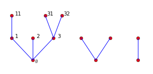 Figure 1
 Figure 2